Constrained Backtracking Matching Pursuit Algorithm for Image Reconstruction in Compressed Sensing

Abstract

Image reconstruction based on sparse constraints is an important research topic in compressed sensing. Sparsity adaptive matching pursuit (SAMP) is a greedy pursuit reconstruction algorithm, which reconstructs signals without prior information of the sparsity level and potentially presents better reconstruction performance than other greedy pursuit algorithms. However, SAMP still suffers from being sensitive to the step size selection at high sub-sampling ratios. To solve this problem, this paper proposes a constrained backtracking matching pursuit (CBMP) algorithm for image reconstruction. The composite strategy, including two kinds of constraints, effectively controls the increment of the estimated sparsity level at different stages and accurately estimates the true support set of images. Based on the relationship analysis between the signal and measurement, an energy criterion is also proposed as a constraint. At the same time, the four-to-one rule is improved as an extra constraint. Comprehensive experimental results demonstrate that the proposed CBMP yields better performance and further stability than other greedy pursuit algorithms for image reconstruction.

1. Introduction

Image reconstruction is a significant application of multimedia signal processing. Compressed sensing (CS) is a technique that reconstructs sparse, compressible signals from under-determined random linear measurements. Over the past few decades, CS has been widely applied to image processing, including image reconstruction [1,2,3,4,5] and acquisition [6,7,8].

Various algorithms have been proposed for CS-based signal reconstruction with sparse constraints [9], which can be categorized into three classes. The first class is the non-convex optimization [10], such as re-weighted $l_1$ norm minimization [11] and $l_q$ norm minimization [12]. However, non-convex optimization is a non-deterministic polynomial (NP)-hard problem, which is hard to solve. The second class focuses on convex optimization based on the minimization of the $l_1$ norm. The basis pursuit (BP) algorithm is typically used for convex optimization, but its $l_1$ norm-based cost function is sometimes not differentiable. It also involves high computational complexity, thus limiting its practical applications [13,14,15].

The third category includes a set of greedy pursuit algorithms, which are to easy implement and have low computational complexity [13,14,15,16,17,18,19,20,21]. Specifically, orthogonal matching pursuit (OMP) [15,16,17], stage-wise OMP (StOMP) [18], and regularized orthogonal matching pursuit (ROMP) [19,20] have been proposed. The reconstruction complexity of basic greedy pursuit algorithms is roughly about O(kMN), which is much lower than that of BP algorithm.

While the greedy pursuit algorithms show superiority in easy implementation and computational efficiency, they typically require additional measurements for reconstruction and lack stable reconstruction capability. The problem is alleviated when backtracking is introduced. For example, the subspace pursuit (SP) algorithm [21] and compressive sampling pursuit (CoSaMP) algorithm [22] have been proposed based on the backtracking scheme. The difference between SP and CoSaMP is that the latter chooses $2k$ indices to combine the estimated support set from the previous iteration. However, it is necessary to estimate the sparsity level of signal k before applying SP and CoSaMP. Indeed, it is impractical to know the accurate sparsity level k of unknown signals in advance.

Then, sparsity adaptive matching pursuit (SAMP), which can recover signals without knowing the sparsity level, was proposed by Do et al. [23]. It alternatively estimates the sparsity level when the residue’s energy increases between two consecutive stages and updates the support set size of the signal using a fixed and small step size. SAMP has apparent advantages when processing one-dimensional sparse signals. However, since one is used as the initial step size, when processing high-dimensional signals, the small step size significantly affects the result and efficiency of reconstruction. To further improve the reconstruction performance, an energy-based adaptive matching pursuit (EAMP) has been proposed [24]. One limitation of EAMP is that it only focuses on the binary signal reconstruction. Rasha et al. used the structured Wilkinson matrix as the measurement matrix to improve the efficiency of SAMP [25]. More recently, the improved generalized sparsity adaptive matching pursuit (IGSAMP) algorithm has been proposed. This algorithm uses a nonlinear step size to approximate the sparsity level, and only a small initial step size can be selected. Meanwhile, it requires carefully choosing the parameters without referring to the sensitivity of a large step size [26].

To improve the reconstruction performance of the sparsity adaptive matching pursuit algorithm and make it less sensitive to the step size, we propose a compositely constrained backtracking matching pursuit (CBMP) algorithm for image reconstruction. The main contributions of this paper are summarized as follows.

(1)

The restricted isometry property (RIP) is analyzed, and the relationship between observed values and signals is derived and demonstrated.

(2)

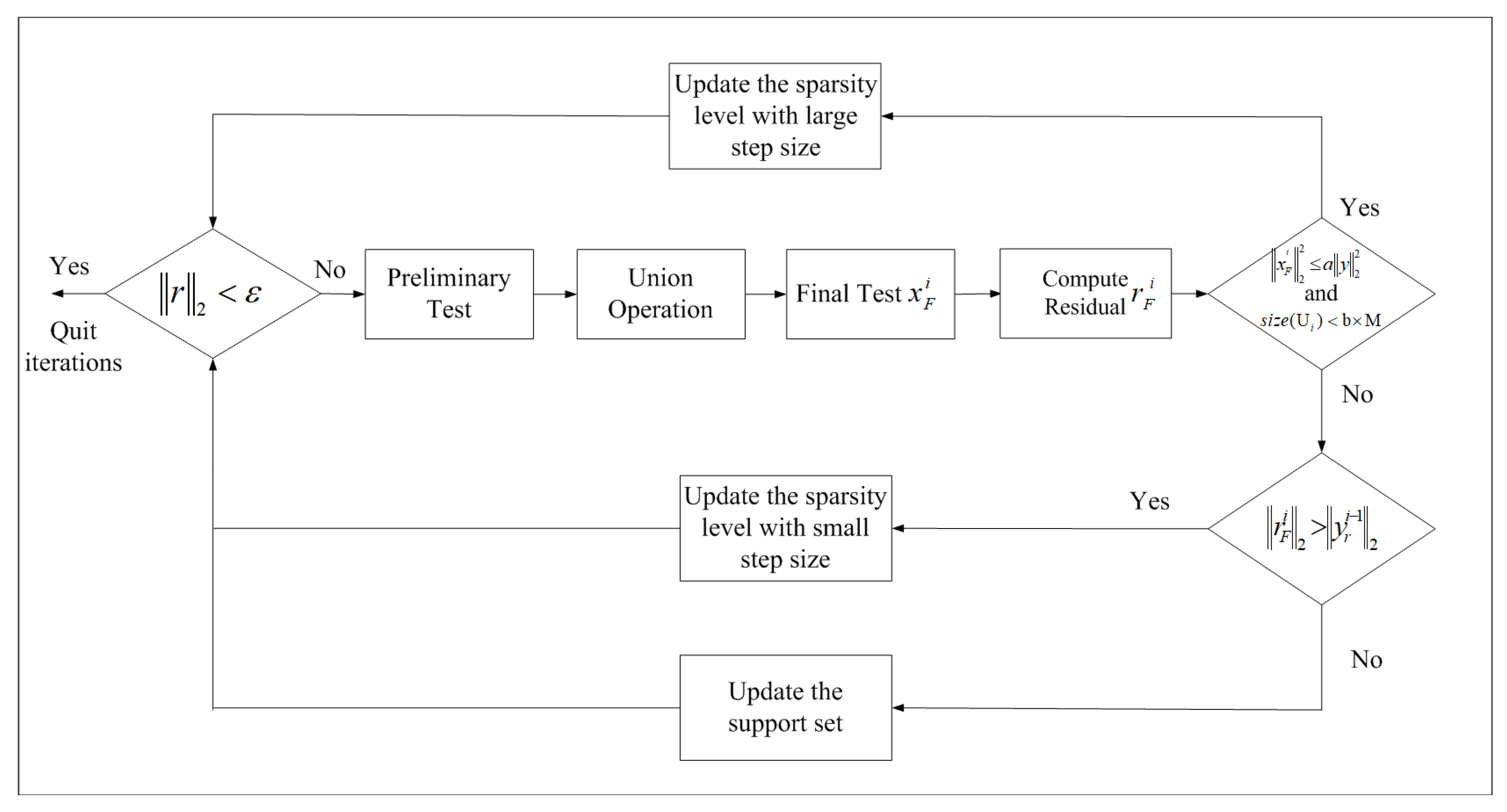
The reconstruction process is divided into three stages, including the large step size stage, small step size stage, and support set update stage. Different step sizes are used in these stages.

(3)

A backtracking threshold operation is proposed, which adopts a composite strategy and uses dedicated parameters to control the different step sizes in the reconstruction process.

(4)

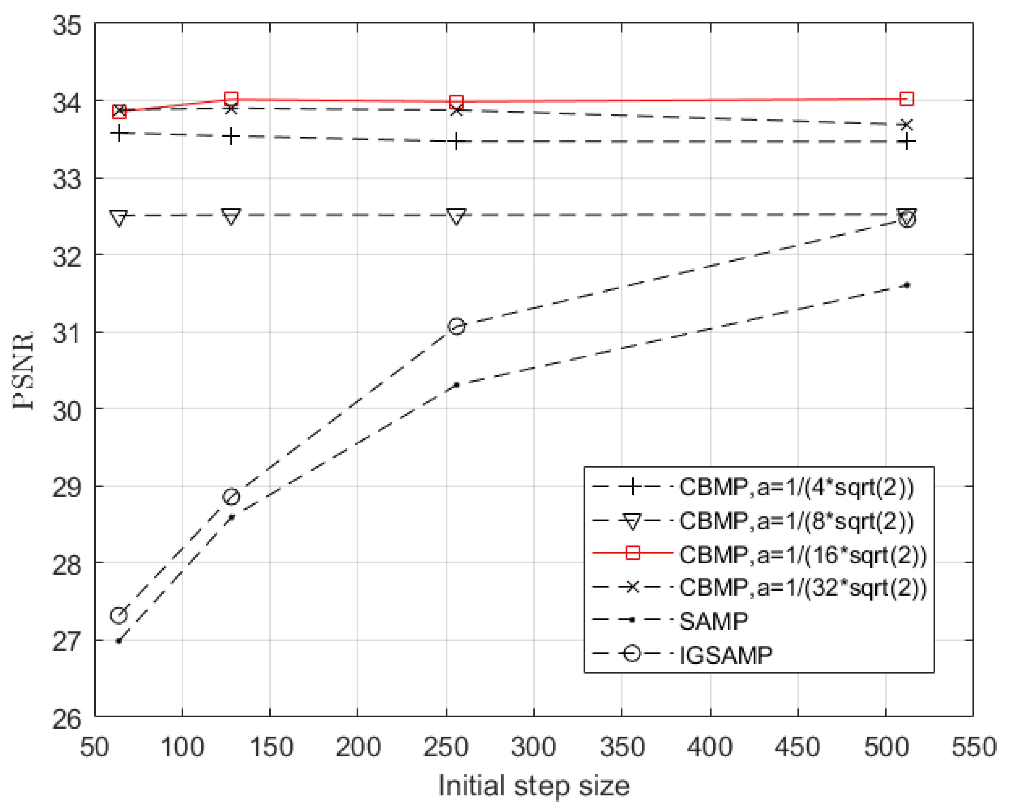
The proposed algorithm can achieve satisfactory reconstruction performance and overcome the sensitivity to step size.

2. Preliminaries

2.1. A Review of Compressed Sensing

CS compresses the signal at the time of sampling while maintaining the ability to reconstruct the original signal. For a signal $x\in {\mathbb{R}}^N$ that has at most k terms as nonzero components in some bases $\Psi$, the compressed signal y is obtained through the following linear transform:

$$y=\Phi \Psi x$$

(1)

where y is an $M\times 1$ vector and $\Phi$ denotes an $M\times N$ random measurement matrix with $M\ll N$.

In general, M is much larger than $N,$ so the reconstruction x from the measurements y can be solved by forming an underdetermined set of linear equations. Thus, the CS reconstruction is generally an ill-posed problem. To guarantee an exact reconstruction of every k sparse signal, one of the most important assumptions of $\mathrm{CS}$ is that the measurement matrix $\Phi$ satisfies the restricted isometry property (RIP) [27,28] with parameters $(k,\delta )$ [29,30,31].

$$\left(1-{\delta }_k\right){\parallel x\parallel }_2^2\le {\parallel \Phi x\parallel }_2^2\le \left(1+{\delta }_k\right){\parallel x\parallel }_2^2$$

(2)

where ${\delta }_k$ is the RIP constant and $0<{\delta }_k<1,k<M$.

When a matrix satisfies the RIP, the lengths of all sufficiently sparse vectors are approximately preserved under the matrix transformation [29]. In [19,21], it was demonstrated that if ${\delta }_{2K}<\sqrt{2}-1$, then the signal can be exactly reconstructed via a finite number of iterations.

The CS reconstruction aims to find the sparsest possible solution that satisfies Equation (1). Then, the CS model [1,31] is represented as:

$${min\parallel \Psi x\parallel }_0\mathrm{subject}\mathrm{to}y=\Phi \Psi x$$

(3)

where ${\parallel \Psi x\parallel }_0$ is the $l_0$ norm and denotes the number of nonzero components in $(\Psi x)$.

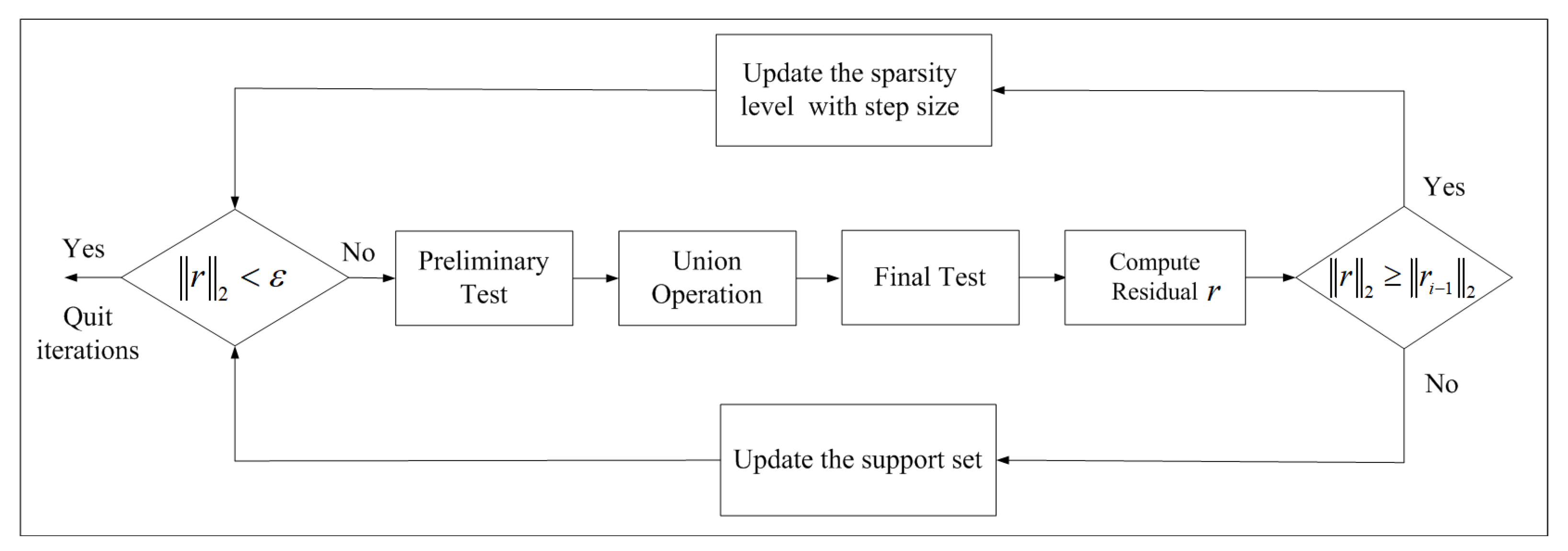
2.2. A Review of the Greedy Pursuit Algorithms

Among the reconstruction algorithms used in CS, the greedy pursuit algorithms are the most widely used due to their easy implementation and low computational complexity.

The goal of greedy pursuit algorithms is to find the support set of the unknown signal. After finding the support set, the signal can be reconstructed by solving a least squares problem [31,32,33]. There exit the indices of the optimal support set $J\in \{1,2,\dots ,n\}$, and $z^{*}$ satisfies $y=z^{*}{\phi }_J$. ${\phi }_J$ is the J-th column (index) of $\Phi$. Then, the error function $e\left(j\right)$ is:

$$\begin{array}{cc}\hfill e\left(j\right)=& \underset{z}{min}{∥z{\phi }_j-y∥}_2^2=\underset{z}{min}\left[\left({\phi }_j^T{\phi }_j\right)z^2-2\left({\phi }_j^{T}y\right)z+y^{T}y\right]\hfill \\ & =\underset{z}{min}\left({\phi }_j^T{\phi }_j\right){\left(z-\frac{{\phi }_j^{T}y}{{\phi }_j^T{\phi }_j}\right)}^2+y^{T}y-\frac{{\left({\phi }_j^{T}y\right)}^2}{{\phi }_j^T{\phi }_j}\hfill \end{array}$$

Letting $e\left(j\right)=0,$ the optimal solution:

$$z^{*}=\left\{\begin{array}{c}\frac{{\phi }_j^{T}y}{{∥{\phi }_j∥}^2},j=J\hfill \\ 0,\mathrm{otherwise}.\hfill \end{array}\right\}$$

(4)

The matching pursuit (MP) algorithm is one of the most classical and primitive greedy pursuit algorithms. As described in Equation (4), only the column J minimizing the error function is selected in each iteration of the MP algorithm [32]. Later on, the OMP algorithm [15] was developed based on the MP algorithm. As stated in OMP, some indices are searched, corresponding to the most significant correlations between the measurement matrix and the residual. In each iteration, only one or more coordinates are selected and added to the support set. These selected coordinates correspond to the columns (indices) of observation matrices with the largest correlation with the residuals. The optimization iterates until the termination condition is satisfied. Finally, the pseudo-inverse of the observation matrix corresponding to the obtained support set is used for signal reconstruction.

CS-based greedy pursuit algorithms adopted in CS include OMP [15,16,17], StOMP [18], ROMP [19,20], SP [21], CoSaMP [22], SAMP [23], EAMP [24], and IGSAMP [26]. Utilizing some criteria, they can approximate the sparse signals iteratively. Each of the algorithms iteratively computes the estimated support set of the signals. In each iteration, one or several coordinates are added to the support set. In particular, in OMP, only one column of $\Phi$ is added to the estimated support set. In StOMP, a hard threshold is used to choose several columns that are to be added to the support set. Both algorithms have to select these columns previously. Otherwise, these algorithms cannot be rectified.

These greedy pursuit algorithms required more measurements for exact reconstruction and lacked stable reconstruction capability until the backtrackingidea was introduced in SP [21] and CoSaMP [22]. Refining the last estimated support set, the backtracking scheme allows eliminating the wrong coordinates, which are selected in the previous iterations. The candidate set is introduced into the greedy pursuit algorithm, which is the key point of the backtracking. However, both SP [21] and CoSaMP [22] require prior knowledge about the sparsity level k, which is impractical to know previously. SAMP [23], on the other hand, was put forward to gradually approach the sparsity level by accumulation with a step size. The SAMP algorithm is shown in Figure 1 and Algorithm 1.

Algorithm 1 Sparsity adaptive matching pursuit algorithm

Input: $M\times N$ measurement matrix $\Phi$, measurement vector y, step size s Initialization: $\widehat{x}=0$ {Trivial Initialization}, $r^0=y$ {Initial residue}, ${\mathrm{U}}^0=\varnothing$ {the estimated support set}, $L=s$ {size of the support set}, $j=1$ { stage index}, $i=1$ { iteration index}. Repeat: 1.    Preliminary test: find the matched L indices from $\Phi$ based on the correlation between $\Phi$ and $r^{i-1}$, that is $D^i=max\left(\right|{\Phi }^T{r}^{i-1}|,L)$. 2.    Make the candidate list: ${\mathrm{U}}^i=T^{i-1}\bigcup D^i,x_{{\mathrm{U}}^i}={\Phi }_{{\mathrm{U}}^i}^{†}y$. 3.    Final test: $\mathrm{F}=max\left(\right|x_{{\mathrm{U}}^i}|,L),x_{\mathrm{F}}={\Phi }_{\mathrm{F}}^{†}y$. 4.    Compute residual: $r=y-{\Phi }_{\mathrm{F}}{x}_{\mathrm{F}}$.         if the halting condition is true, then quit the iteration;         else if ${\parallel r\parallel }_2\ge {\parallel r_{i-1}\parallel }_2$, then         $j=j+1$ {update the stage index}, $L=j\times s$ {update the size of support set};         else ${\mathrm{T}}^i=\mathrm{F}$ {update the support set}, $r^i=r$ { update the residual}, $i=i+1$.         end if         Until the halting condition is true; Output:$\widehat{x}={\Phi }_{\mathrm{T}}^{†}y$ {update the stage index}, $L=j\times s$ {a sparse reconstruction computed by the least squares algorithm}

SAMP uses the “divide and conquer” principle stage-by-stage to estimate the sparsity level and the true support set of the target signals. SAMP applies two tests, namely the preliminary test and the final test, to estimate the signal’s support set. The preliminary test is used to implement the selection of the L largest elements corresponding to the most considerable correlation between the residual and the measurement matrix, denoted by $D^i=max\left({\Phi }^T{\mathrm{r}}^{i-1}\mid ,L\right)$. After the preliminary test, a candidate list $\mathrm{U}$ is created by the union of the chosen list in the preliminary test and the support set in the previous iteration, represented by ${\mathrm{U}}^i=T^{i-1}\cup D^i.$ The final test firstly solves a least squares problem to obtain $x_{{\mathrm{U}}^i},$ and then chooses a subset of the L largest elements from $x_{{\mathrm{U}}^i}$. This subset of coordinates serves as the support set of the current iteration. The residual is finally updated by subtracting the measured vector y from its projection onto the subspace spanned by the columns in the support set. The pseudo-code of SAMP is summarized below.

${\Phi }^{†}={\left({\Phi }^T\Phi \right)}^{-1}{\Phi }^T$ represents the pseudo-inverse of $\Phi ,$ in which ${\Phi }^T$ denotes the transposition of $\Phi$. The main innovation of SAMP is that the increment of the residual is used as the criterion to judge the sparsity level by accumulating with the step size. As previously mentioned, SAMP uses a fixed step size that is sensitive to the reconstruction performance [23]. Specifically, when SAMP is applied to two-dimensional images, the selection of the step size seriously affects the image reconstruction performance due to the lack of flexibility and adaptation in the sparsity level update stage. As shown in Figure 2, the reconstruction performance is affected by the step size. When the step size $s=64,$ the peak signal-to-noise ratio (PSNR) is $24.04\mathrm{dB}$, whereas when $s=512,$ the PSNR is $28.44\mathrm{dB}$.

Then, a variable step size was proposed in EAMP [24], but it focuses on one-dimensional sparse binary signal reconstruction. Recently, IGSAMP [26] was proposed to improve SAMP. Furthermore, it requires one to carefully choose the parameters and control the variable nonlinear step size in the reconstruction process and does not refer to the sensitivity to the step size. In this paper, we propose an improved adaptive greedy algorithm, whose signal reconstruction performance is relatively insensitive to the step size.

3. The Constrained Backtracking Matching Pursuit Algorithm for Image Reconstruction

To overcome the sensitivity to the step size and improve the reconstruction performance of greedy pursuit algorithms, we propose the CBMP algorithm, which introduces restrictions to the backtracking stage, which provides more flexibility as the algorithm gradually approaches the true sparsity level of the unknown signal. The main steps of CBMP are described as follows:

Considering the signal to be reconstructed is a two-dimensional image, the sparsity level is relatively large; the process of sparsity level estimation is divided into large and small step size estimation stages. In the large step size stage, the increment of the step size is $s^j=2\times s^{j-1}$. j denotes the stage iteration index. The increment of the sparsity level in the stage of the small step size is fixed and equals the step size of the previous stage.

Due to the advantages of combing information and improving accuracy [34,35], a composite strategy is proposed to effectively control the increment of the estimated sparsity level in the two stages. It includes two constraints controlled by parameters a and b, which are required in the backtracking threshold operation of CBMP, as described in Algorithm 2. The theoretical support for the composite strategy is clarified as follows:

Theorem 1.

Let $x\in R^N$ be a sparse signal and y be a measurement vector. If the measurement matrix Φ satisfies the RIP, then ${\parallel x\parallel }_2^2>\frac{1}{\sqrt{2}}{\parallel y\parallel }_2^2.$ The proof is presented in Appendix A.

Algorithm 2 The proposed CBMP algorithm

Input: $M\times N$ measurement matrix $\Phi ,$ measurement vector $y,$ step size $s^0$ Initialization: $x=0$ {trivial Initialization}; $y_r^0=y$ {initial residue}; $T^0=\varnothing$ {the estimated support set}; $L^0=s^0$ {size of the support set (sparsity level)}; $j=1$ {stage index}; i = 1 {$iterationindex$}; ${\mathrm{U}}^0=\varnothing$ {union set} Repeat the following steps until the stopping condition holds: 1.   Preliminary test: $v={\Phi }^T{y}_r^{i-1},$ find the matched set $D^i=\left\{L^{j-1}\right.$ indices corresponding to the largest absolute values of $v\},$ that is $\left.D^i=max\left(|{\Phi }^T{y}_r^{i-1}\right|,L^{j-1}\right)$. 2.   Union operation: to broaden the selection space and make candidate list ${\mathrm{U}}^i:{\mathrm{U}}^i=T^{i-1}\cup D^i,x_{{\mathrm{U}}^i}={\Phi }_{{\mathrm{U}}^i}^{†}y$. 3.   Final test: to obtain the vector $x_F^i:$ find the matched indices $F^i$ based on the largest absolute values of $x_{{\mathrm{U}}^i},$ that is $F^i=max\left(\left|x_{{\mathrm{U}}^i}\right|,L^{j-1}\right),x_F^i={\Phi }_{F^i}^{†}y$. 4.   Compute residual: $r_F^i=y-{\Phi }_F{x}_F^i$. 5.   Backtracking threshold operation:       if ${∥x_F^i∥}_2^2\le a{\parallel y\parallel }_2^2$ and $size\left({\mathrm{U}}_i\right)<b\times M$, then shift into the large step size estimation stage: $s^j=2\times s^{j-1},L^j=L^{j-1}+s^j,y_r^i=y_r^{i-1},j=j+1,i=i+1$, then shift into 1.       if ${∥r_F^i∥}_2>{∥y_r^{i-1}∥}_2$, then shift into the small step size estimation stage: $s^j=s^{j-1},L^j=L^{j-1}+s^j,y_r^i=y_r^{i-1},j=j+1,i=i+1$, then shift into 1.      Otherwise, shift into the stage that updates the support set based on the current estimated sparsity level: $y_r^i=r_F^i,L^j=L^{j-1},T^i=F^i,i=i+1$, then shift into 1. Output:$x={\Phi }_T^{†}y${a sparse reconstruction computed by the least squares algorithm}

According to Theorem 1, the energy of the original signal x is greater than the square root of one half of that of the measurement vector $y,$ that is ${\parallel x\parallel }_2^2>\frac{1}{\sqrt{2}}{\parallel y\parallel }_2^2$. Different step sizes are used in CBMP. Specifically, the estimated sparsity level is far smaller than the true one at the early stage. Based on this theorem, the energy criterion can be improved by introducing a parameter a to constrain the reconstruction stages.

Inspired by the “four-to-one” practical rule proposed in [27], the measurement number should be four-times the signal sparsity level for signal reconstruction. In CBMP, ${\mathrm{U}}_i$ is the union of a new matched set and the estimated support set of the previous iteration. M is the row number of the measurement matrix. We introduce the “four-to-one” rule to CBMP and use the parameter b to constrain the estimation stage. The relationship between the parameters a and b is analyzed in Section 4.

Figure 3 shows the flowchart of the CBMP algorithm. The reconstruction process is divided into the sparsity level update stage and the support set update stage. As for the details, the sparsity level update stage includes both the large and small step size update stages. In the early stage of reconstruction, the estimated sparsity level is far less than the true one, so large step sizes are adopted to estimate the sparsity level. As the iteration goes on, after the threshold condition is satisfied, it enters a small step size stage. The reason why CBMP can achieve better reconstruction performance than SAMP is attributed to its superior capability in handling the wrong indices (atoms). When the current obtained sparsity level is far less than the true one, those false indices can be easily added into the candidate support set. However, these false indices are difficult to eliminate in the later iteration. Therefore, at the beginning of the iteration, a large step size allows those false indices to be filtered out.

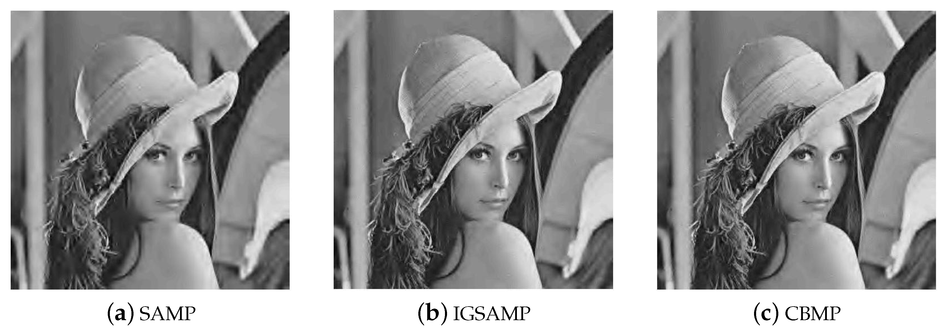
4. Experimental Results

Several experiments were conducted to illustrate the performance of the CBMP algorithm. The proposed CBMP was compared with SAMP [23] and IGSAMP [26]. The halting condition used by these algorithms was $∥y_r∥⩽{10}^{-5}$. For a fair comparison, the same initial step size was used by CBMP, SAMP, and IGSAMP. It should be noted that in SAMP and IGSAMP, the reconstruction results shown in their simulation experiments [23,26] are obtained by a small step size (s = 1). In practical applications, when two-dimensional images are stacked into long one-dimensional vectors, the sparsity level in the transform domain is far greater than one. Correspondingly, the step sizes of the proposed algorithm were relatively large. The step sizes used in the experiment were 64, 128, 256, and 512, respectively. Different sampling rates were used to demonstrate the reconstruction performance of CBMP. The wavelet transform was chosen as the sparse basis to represent images. The quality of recovered images was measured by the peak signal-to-noise ratio (PSNR), which is expressed as:

$$\mathrm{MSE}=\frac{1}{M\times N}\sum _{i=0}^{M-1}\sum _{j=0}^{N-1}{|I(i,j)-\widehat{I}(i,j)|}^2$$

(5)

$$\mathrm{PSNR}(I,\widehat{I})=10{log}_{10}\left(\frac{\mathrm{MAX}}{\mathrm{MSE}}\right)$$

(6)

where $M=N=512$, $I(i,j)$ denotes the original value of the test image at the position $(i,j)$ and $\widehat{I}(i,j)$ denotes the reconstructed value at the position $(i,j)$. The maximum pixel intensity is given as MAX. All images here are expressed using 8 bit intensity values per pixel, so the peak intensity is 255. The experiment configuration is as follows: the CPU was an Intel^® Core™ i5-7200U at 2.50 GHz, and the size of the RAM was 8 GB. The programming language used to perform the experiments was MATLAB. Several experiments were conducted to validate the advantages of CBMP.

According to Theorem 1, ${\parallel x\parallel }_2^2>\frac{1}{\sqrt{2}}{\parallel y\parallel }_2^2$. In CBMP, $x_F$ should gradually approach the true one and $x_F$ is much smaller than x at the beginning. Simultaneously, there are two update stages, and then, the threshold parameter a is contracted within $\frac{1}{4\sqrt{2}}\left(\frac{1}{2}\times \frac{1}{2}\times \frac{1}{\sqrt{2}}\right)$. Our experiments demonstrate that the threshold parameters a and b do not distinctively affect the reconstruction performance if the parameter satisfies $a\le \frac{1}{4\sqrt{2}}.$ In CBMP, the support set of the signal obtained by the current iteration is constrained by the parameter a in the step size update stage, while ${\mathrm{U}}_i$ is the union of the estimated support set of the previous iteration and the currently selected support set. Therefore, the relationship between these two parameters is set as $b=2a$. These two parameters play different roles, as a is used after the final test, while b corresponds to the union operation after the preliminary test.

The relationship between the threshold parameters and reconstruction performance is shown in Figure 4 and Figure 5. Meanwhile, SAMP and IGSAMP are both tested. Two standard images, “Lena” and “Peppers”, were reconstructed to test the reconstruction performance of different parameter pairs $(a,b).$ For a fair comparison, the sampling rate was 0.4, and the same initial step sizes were used. The initial step sizes were chosen from 64 to 512. From Figure 4, we can see that the reconstruction performance of CBMP with different threshold parameters is better than that of SAMP and IGSAMP. For example, when $a=\frac{1}{16\sqrt{2}}$, all the PSNR values of CBMP with different initial step sizes are greater than $33.5.$ While the initial step size is $512,$ SAMP achieves the maximum PSNR value, which is less than $32,$ and IGSAMP offers the maximum PSNR value, which is less than $32.5.$ Therefore, CBMP offers better reconstruction performance than SAMP and IGSAMP. From Figure 5, it is noticed that if $a\le \frac{1}{4\sqrt{2}},$ all the PSNR values of CBMP with different step sizes are greater than $31.$ Therefore, the introduction of the threshold operation is necessary for the improvement of greedy pursuit algorithms. At the same time, threshold parameters do not distinctively affect the reconstruction performance if they are satisfied with the constrained condition in CBMP. Meanwhile, the reconstruction performance of CBMP with $a=\frac{1}{16\sqrt{2}}$ is better than the others; thus, this a value is regarded as the optimal value in the CBMP.

Table 1. PSNR (dB) comparison of the Lena image when the sampling ratio is 0.3.

Initial Step Size	PSNR of SAMP	PSNR of IGSAMP	PSNR of CBMP
64	25.45	26.23	32.13
128	26.41	28.45	31.91
256	27.62	29.89	31.87
512	28.98	31.76	31.83

and

Table 2. PSNR (dB) comparison of the Lena image when the sampling ratio is 0.4.

Initial Step Size	PSNR of SAMP	PSNR of IGSAMP	PSNR of CBMP
64	26.99	27.32	33.85
128	28.59	28.86	34.01
256	30.31	31.07	33.99
512	31.60	32.46	34.02

compare CBMP, SAMP, and IGSAMP in terms of the reconstruction performance (PSNR) on the Lena image with different sampling ratios and initial step sizes.

Table 3. PSNR (dB) comparison of the Peppers image when the sampling ratio is 0.3.

Initial Step Size	PSNR of SAMP	PSNR of IGSAMP	PSNR of CBMP
64	24.04	25.33	31.46
128	25.19	27.85	31.42
256	26.87	30.54	31.40
512	28.44	31.10	31.38

and

Table 4. PSNR (dB) comparison of the Peppers image when the sampling ratio is 0.4.

Initial Step Size	PSNR of SAMP	PSNR of IGSAMP	PSNR of CBMP
64	26.30	25.37	32.80
128	28.00	27.96	32.81
256	28.87	30.79	32.81
512	30.67	32.75	32.84

compare CBMP, SAMP, and IGSAMP in terms of the reconstruction performance (PSNR) on the Peppers image with different sampling ratios and initial step sizes.

In Table 1, when the sampling ratio is 0.3, each PSNR value of the CBMP algorithm is greater than that of SAMP and IGSAMP. For example, with the initial step size of 64, the PSNR value of SAMP and IGSAMP is 25.45 dB and 26.23 dB, respectively, but the PSNR value of CBMP is 32.13 dB. Table 2 shows the PSNR values of SAMP, IGSAMP, and CBMP with the same sampling ratio of 0.4. Different step sizes are used. The PSNR values of SAMP with different initial step sizes range from 26.99 dB to 31.60 dB. The PSNR values of IGSAMP are increased from 27.32 dB to 32.46 dB. However, the PSNR values of CBMP are greater than those of SAMP and IGSAMP, achieving 33.9675 dB as the average value.

Similarly, Table 3 shows the PSNR values of the Peppers image by SAMP, IGSAMP, and CBMP when the sampling ratio is 0.3. Each PSNR value of the CBMP algorithm is greater than that of SAMP and IGSAMP. Table 4 shows the PSNR values of the Peppers image by SAMP, IGSAMP, and CBMP when the sampling ratio is 0.4. Different step sizes are used. For example, as the initial step size is 512, the PSNR value of SAMP and IGSAMP is 30.67 dB and 32.75 dB, respectively, while the PSNR value of CBMP is 32.84 dB.Therefore, CBMP can achieve better reconstruction performance with different sampling ratios and initial step sizes.

Finally, the reconstructed results of the Lena image using SAMP, IGSAMP, and CBMP are shown in Figure 6 and Figure 7. The sampling rate is 0.3; different step sizes are used. The reconstructed results of the Peppers image using SAMP, IGSAMP, and CBMP are shown in Figure 8 and Figure 9.

In our test, CBMP outperforms SAMP and IGSAMP in terms of visual effect and PSNR, which is irrelevant to the setup of the initial step size value. At the same time, with different step sizes, the reconstruction performance of CBMP is stable. For example, Figure 8a and Figure 9a show different visual reconstruction effects when the initial step size is 64 and 512, individually, and the same conclusion can be made from Figure 8b and Figure 9b. It is noted that the visualization effect is not obvious in Figure 8c and Figure 9c when the initial step size is 64 and 512, respectively. Therefore, it can be concluded that the CBMP algorithm is relatively insensitive to the step size.

5. Conclusions

In this paper, a constrained backtracking matching pursuit algorithm is proposed for image reconstruction using compressed sensing. A composite strategy, including two constraints, is adopted to effectively control the estimated sparsity level’s increment at different stages and accurately estimate the true support set of the image to be reconstructed. On the one hand, the energy criterion between the estimated signal and the measurement is used as a constraint. On the other hand, the four-to-one practical rule is considered and improved as another control. Due to the introduction of these composite mechanisms, the reconstruction performance of the proposed algorithm outperforms the greedy pursuit algorithms, including SAMP and IGSAMP. In particular, CBMP offers a stable reconstruction performance, which is insensitive to the initial step size. In our future works, the CBMP algorithm will be applied to neural network framework-based signal reconstruction, including medical image reconstruction.

References

1. Candès, E.J.; Romberg, J.; Tao, T. Robust uncertainty principles: Exact signal reconstruction from highly incomplete frequency information. IEEE Trans. Inf. Theory 2006, 5, 489–509. [Google Scholar] [CrossRef] [Green Version]
2. Wei, Z.R.; Zhang, J.L.; Xu, Z.Y.; Liu, Y. Optimization methods of compressively sensed image reconstruction based on single-pixel imaging. Appl. Sci. 2020, 10, 3288. [Google Scholar] [CrossRef]
3. Hashimoto, F.; Ote, K.; Oida, T.; Teramoto, A.; Ouchi, Y. Compressed sensing magnetic resonance image reconstruction using an iterative convolutional neural network approach. Appl. Sci. 2020, 10, 1902. [Google Scholar] [CrossRef] [Green Version]
4. Jiang, M.F.; Lu, L.; Shen, Y.; Wu, L.; Gong, Y.L.; Xia, L.; Liu, F. Directional tensor product complex tight framelets for compressed sensing MRI reconstruction. IET Image Process. 2019, 13, 2183–2189. [Google Scholar] [CrossRef]
5. Zhang, Z.M.; Liu, X.W.; Wei, S.S.; Gan, H.P.; Liu, F.F.; Li, Y.W.; Liu, C.Y.; Liu, F. Electrocardiogram reconstruction based on compressed sensing. IEEE Access 2019, 7, 37228–37237. [Google Scholar] [CrossRef]
6. Bi, X.; Chen, X.D.; Zhang, Y. Image compressed sensing based on wavelet transform in contourlet domain. Signal Process. 2011, 91, 1085–1092. [Google Scholar] [CrossRef]
7. Ye, J.C. Compressed sensing MRI: A review from signal processing perspective. BMC Biomed. Eng. 2019, 1, 8. [Google Scholar] [CrossRef] [Green Version]
8. Sandino, C.M.; Cheng, J.Y.; Chen, F.; Mardani, M.; Pauly, J.M.; Vasanawala, S.S. Compressed sensing: From research to clinical practice with deep neural networks: Shortening scan times for magnetic resonance imaging. IEEE Signal Process. Mag. 2020, 37, 117–127. [Google Scholar] [CrossRef]
9. Iwen, M.A.; Spencer, C.V. A note on compressed sensing and the complexity of matrix multiplication. Inf. Process. Lett. 2012, 109, 468–471. [Google Scholar] [CrossRef] [Green Version]
10. Chartrand, R.; Staneva, V. Restricted isometry properties and nonconvex compressive sensing. Inverse Probl. 2008, 24, 1–14. [Google Scholar] [CrossRef] [Green Version]
11. Candès, E.J.; Wakin, M.B.; Boyd, S.P. Enhancing sparsity by reweighted l1 minimization. J. Fourier Anal. Appl. 2008, 14, 877–905. [Google Scholar] [CrossRef]
12. Foucart, S.; Lai, M.J. Sparsest solutions of underdetermined linear systems via lq minimization for 0 < q <= 1. Appl. Comput. Harmon. Anal. 2009, 26, 395–407. [Google Scholar]
13. Nam, N.; Needell, D.; Woolf, T. Linear Convergence of Stochastic Iterative Greedy Algorithms with Sparse Constraints. IEEE Trans. Inf. Theory 2017, 63, 6869–6895. [Google Scholar]
14. Tkacenko, A.; Vaidyanathan, P.P. Iterative greedy algorithm for solving the FIR paraunitary approximation problem. IEEE Trans. Signal Process. 2006, 54, 146–160. [Google Scholar] [CrossRef] [Green Version]
15. Tropp, J.A.; Gilbert, A.C. Signal recovery from random measurements via orthogonal matching pursuit. IEEE Trans. Inf. Theory 2007, 5, 4655–4666. [Google Scholar] [CrossRef] [Green Version]
16. Li, H.; Ma, Y.; Fu, Y. An improved RIP-based performance guarantee for sparse signal recovery via simultaneous orthogonal matching pursuit. Signal Process. 2017, 144, 29–35. [Google Scholar] [CrossRef]
17. Needell, D.; Vershynin, R. Greedy signal recovery and uncertainty principles. Proc. SPIE 2008, 6814, 68140J. [Google Scholar]
18. Donoho, D.L.; Tsaig, Y.; Starck, J.L. Sparse solution of under-determined linear equations by stage-wise orthogonal matching pursuit. IEEE Trans. Inf. Theory 2006, 58, 1094–1121. [Google Scholar] [CrossRef]
19. Needell, D.; Vershynin, R. Signal recovery from incomplete and inaccurate measurements via regularized orthogonal matching pursuit. IEEE J. Sel. Top. Signal Process. 2010, 4, 310–316. [Google Scholar] [CrossRef] [Green Version]
20. Zhang, H.F.; Xiao, S.G.; Zhou, P. A matching pursuit algorithm for backtracking regularization based on energy sorting. Symmetry 2020, 12, 231. [Google Scholar] [CrossRef] [Green Version]
21. Dai, W.; Milenkovic, O. Subspace pursuit for compressive sensing signal reconstruction. IEEE Trans. Inf. Theory 2009, 55, 2230–2249. [Google Scholar] [CrossRef] [Green Version]
22. Needell, D.; Tropp, J.A. CoSaMP: Iterative Signal Recovery from Incomplete and Inaccurate Samples. Appl. Comput. Harmon. Anal. 2009, 26, 301–321. [Google Scholar] [CrossRef] [Green Version]
23. Do, T.T.; Gan, L.; Nguyen, N.; Tran, T.D. Sparsity adaptive matching pursuit algorithm for practical compressed sensing. In Proceedings of the 42nd Asilomar Conference on Signals, Systems, and Computers, Pacific Grove, CA, USA, 26–29 October 2008; pp. 581–587. [Google Scholar]
24. Bi, X.; Chen, X.D.; Leng, L. Energy-based adaptive matching pursuit algorithm for binary sparse signal reconstruction in compressed sensing. Signal Image Video Pocess. 2014, 8, 1039–1048. [Google Scholar] [CrossRef]
25. Shoitan, R.; Nossair, Z.; Ibrahim, I.I.; Tobal, A. Improving the reconstruction efficiency of sparsity adaptive matching pursuit based on the Wilkinson matrix. Front. Inf. Technol. Electron. Eng. 2018, 19, 503–512. [Google Scholar] [CrossRef]
26. Zhao, L.Q.; Ma, K.; Jia, Y.F. Improved generalized sparsity adaptive matching pursuit algorithm based on compressive sensing. J. Electr. Comput. Eng. 2020, 4, 1–11. [Google Scholar]
27. Candès, E.J.; Wakin, M.B. An introduction to compressive sampling. IEEE Signal Process. Mag. 2008, 25, 21–30. [Google Scholar] [CrossRef]
28. Kutyniok, G.; Eldar, Y.C. Compressed Sensing: Theory and Applications; Cambridge University Press: Cambridge, UK, 2012. [Google Scholar]
29. Baraniuk, R.; Davenport, M.; DeVore, R.; Wakin, M. A simple proof of the restricted isometry property for random matrices. Constr. Approx. 2008, 28, 253–263. [Google Scholar] [CrossRef] [Green Version]
30. Candès, E.J. The restricted isometry property and its implications for compressed sensing. Comptes Rendus Math. 2008, 346, 589–592. [Google Scholar] [CrossRef]
31. Needell, D. Topics in Compressed Sensing. Ph.D. Dissertation, University of California, Berkeley, CA, USA, 2009. [Google Scholar]
32. Mallat, S.G.; Zhang, Z. Matching pursuits with time-frequency dictionaries. IEEE Trans. Signal Process. 1993, 41, 3397–3415. [Google Scholar] [CrossRef] [Green Version]
33. Elad, M. Sparse and Redundant Representations—From Theory to Applications in Signal and Image Processing; Springer: New York, NY, USA, 2010. [Google Scholar]
34. Leng, L.; Zhang, J.S.; Khan, M.K.; Chen, X.; Alghathbar, K. Dynamic weighted discrimination power analysis: A novel approach for face and palmprint recognition in DCT domain. Int. J. Phys. Sci. 2010, 5, 2543–2554. [Google Scholar]
35. Leng, L.; Li, M.; Kim, C.; Bi, X. Dual-source discrimination power analysis for multi-instance contactless palmprint recognition. Multimed. Tools Appl. 2017, 76, 333–354. [Google Scholar] [CrossRef]
Figure 1. The pipeline of sparsity adaptive matching pursuit (SAMP) [23].
Applsci 11 01435 g001
Figure 2. Performance of SAMP vs. different step sizes.
Applsci 11 01435 g002
Figure 3. The flowchart of the constrained backtracking matching pursuit (CBMP) algorithm.
Applsci 11 01435 g003
Figure 4. PSNR (dB) under different initial step sizes of the Lena image.
Applsci 11 01435 g004
Figure 5. PSNR (dB) under different initial step sizes of the Peppers image.
Applsci 11 01435 g005
Figure 6. Reconstructed results of the Lena image by SAMP, IGSAMP, and CBMP with the initial step size of 64.
Applsci 11 01435 g006
Figure 7. Reconstructed results of the Lena image by SAMP, IGSAMP, and CBMP with the initial step size of 512.
Applsci 11 01435 g007
Figure 8. Reconstructed results of the Peppers image by SAMP, IGSAMP, and CBMP with the initial step size of 64.
Applsci 11 01435 g008
Figure 9. Reconstructed results of the Peppers image by SAMP, IGSAMP, and CBMP with the initial step size of 512.
Applsci 11 01435 g009