
CDL-GAN: Contrastive Distance Learning Generative Adversarial Network for Image Generation


Abstract
1. Introduction
- We propose a comprehensive and effective approach as Contrastive Distance Learning (CDL) to train GAN. This method can be easily extended into different GAN models without any other modification of the backbone.
- We subtly integrate the Siamese modules into the GAN framework with a low computational cost. With its superiority, we alleviate the antagonism between the generator and the discriminator.
- We conduct extensive experiments on three public datasets and demonstrate the versatility of our approach. The results show that CDL can not only address some existing issues in both the generator and discriminator, but also boost the visual quality of the generated images.
2. Preliminaries and Related Works
2.1. Regularizations for GANs
2.2. Characteristic Function Distance for GANs
2.3. Siamese Network
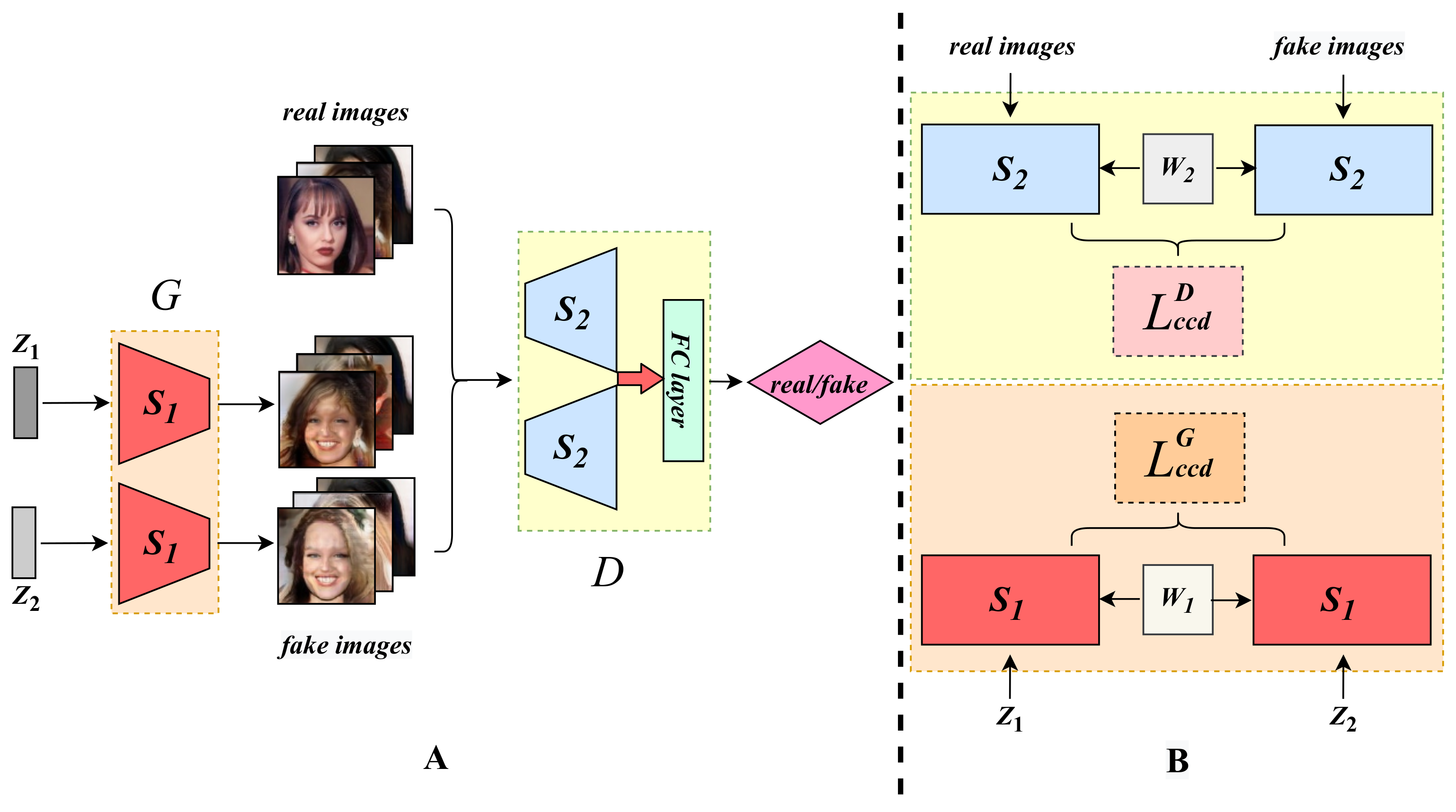
3. Methodology: Contrastive Distance Learning
3.1. Consistent Contrastive Distance
3.2. Characteristic Contrastive Distance
3.3. Enhancement with the Siamese Modules
| Algorithm 1 Contrastive Distance Learning (CDL) |
|
4. Experiments
4.1. Settings and Evaluation Metrics
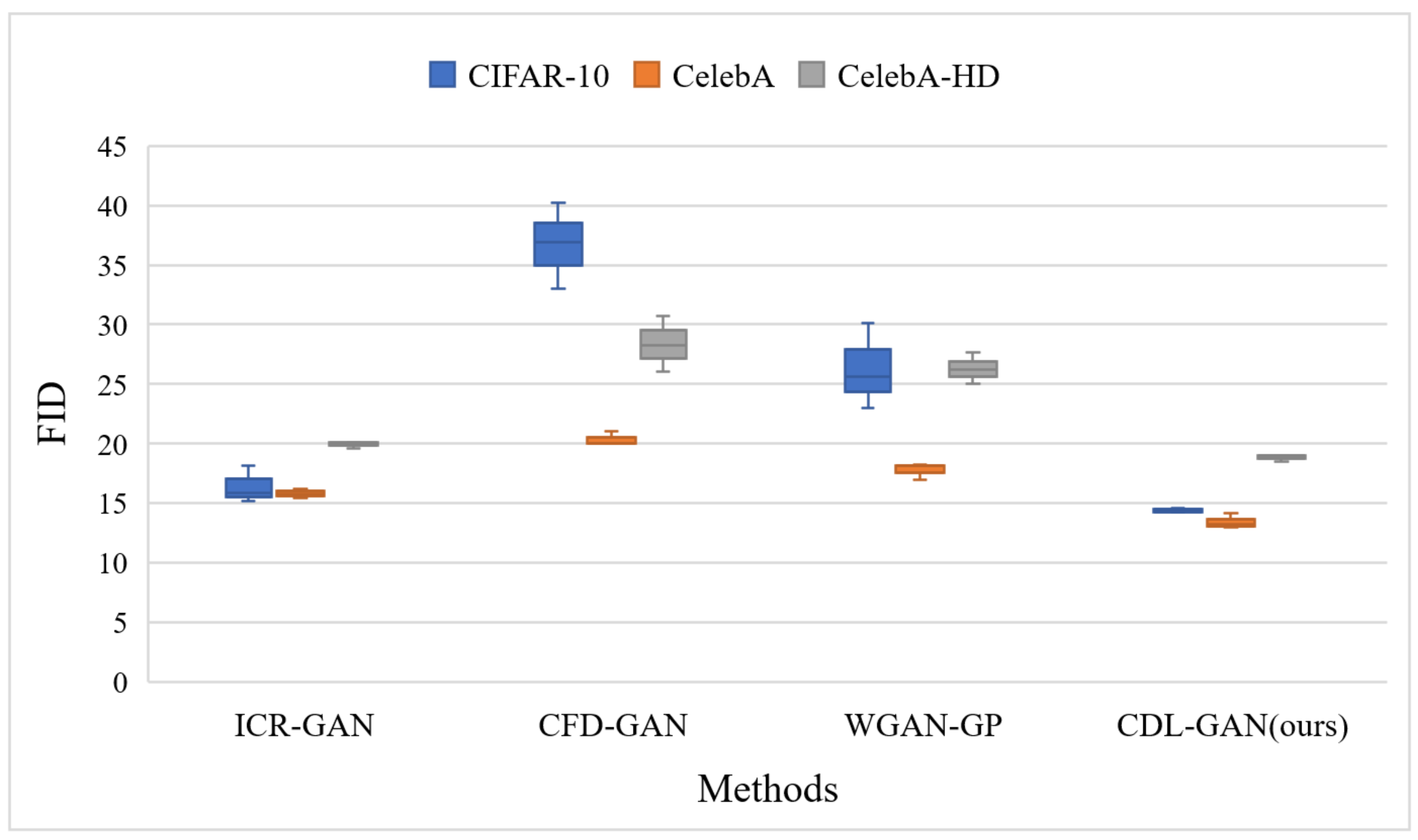
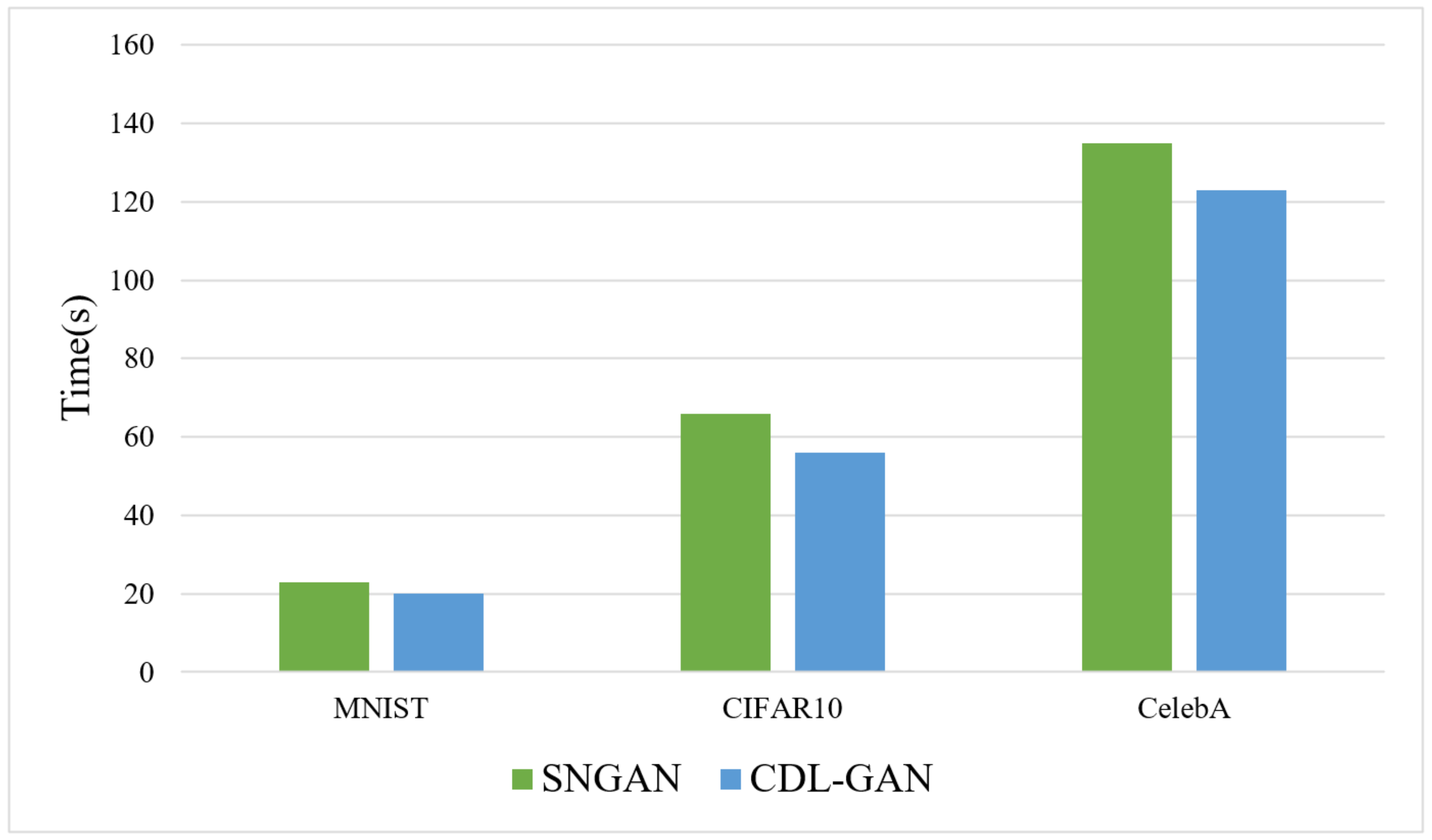
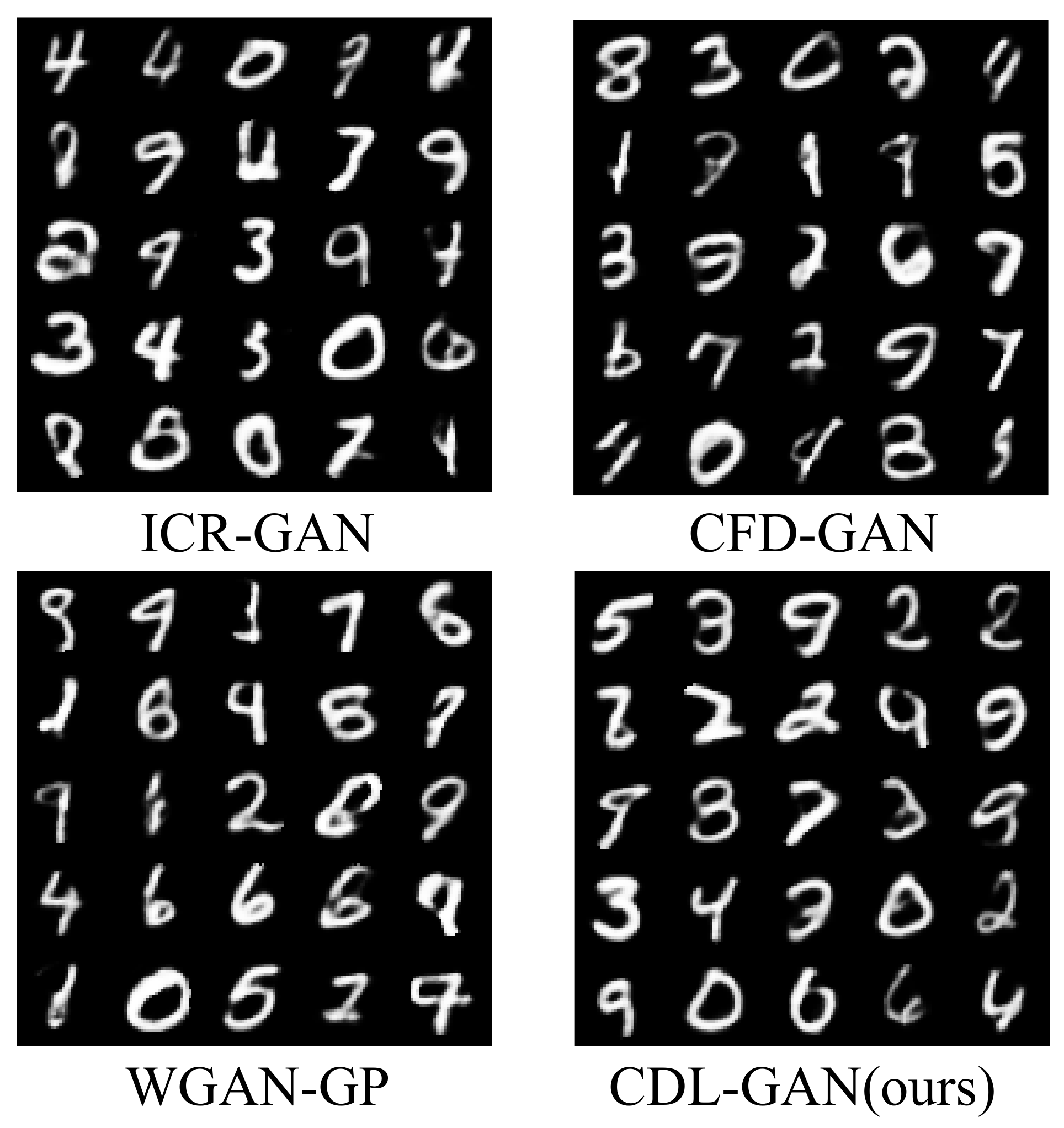
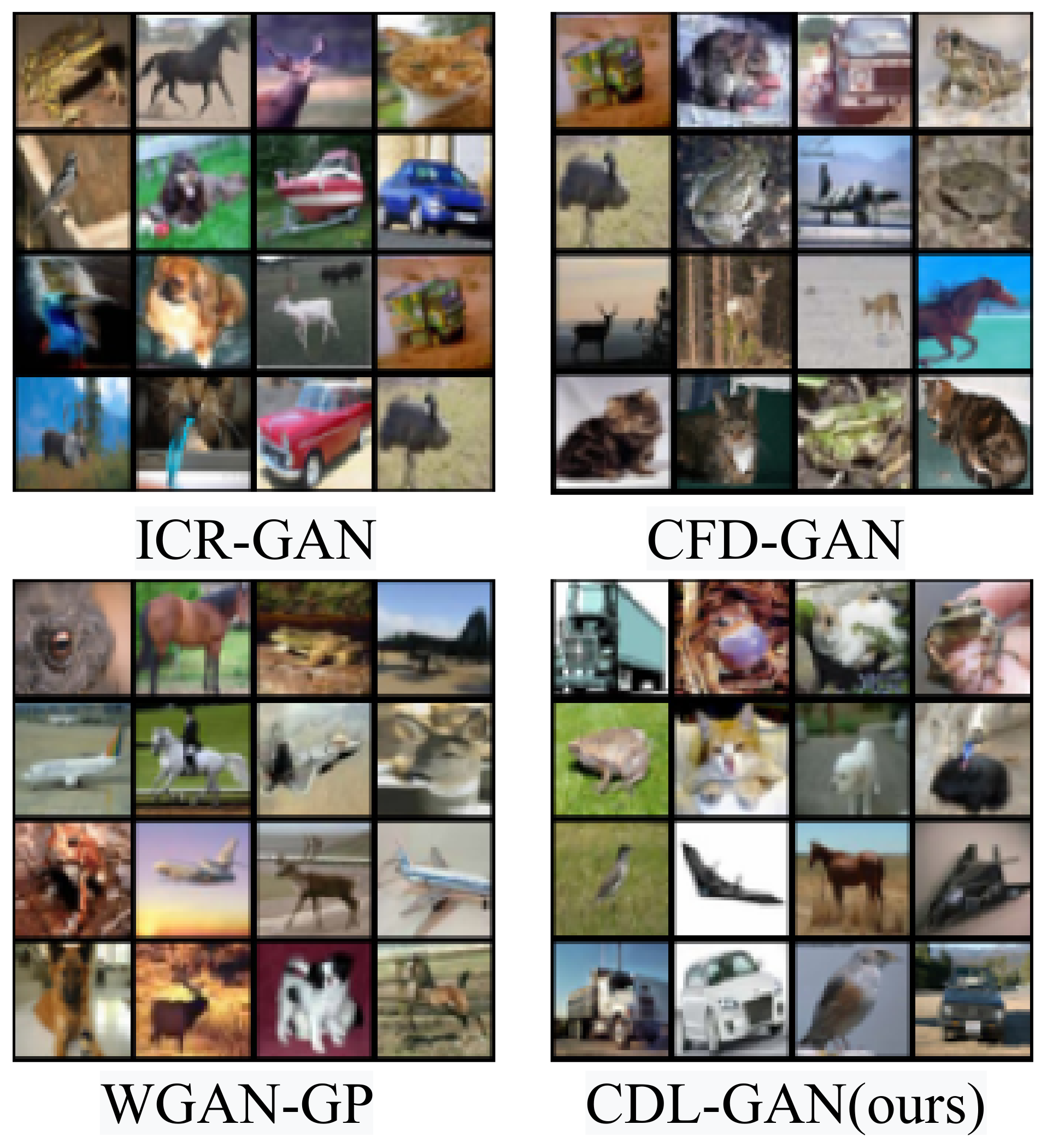
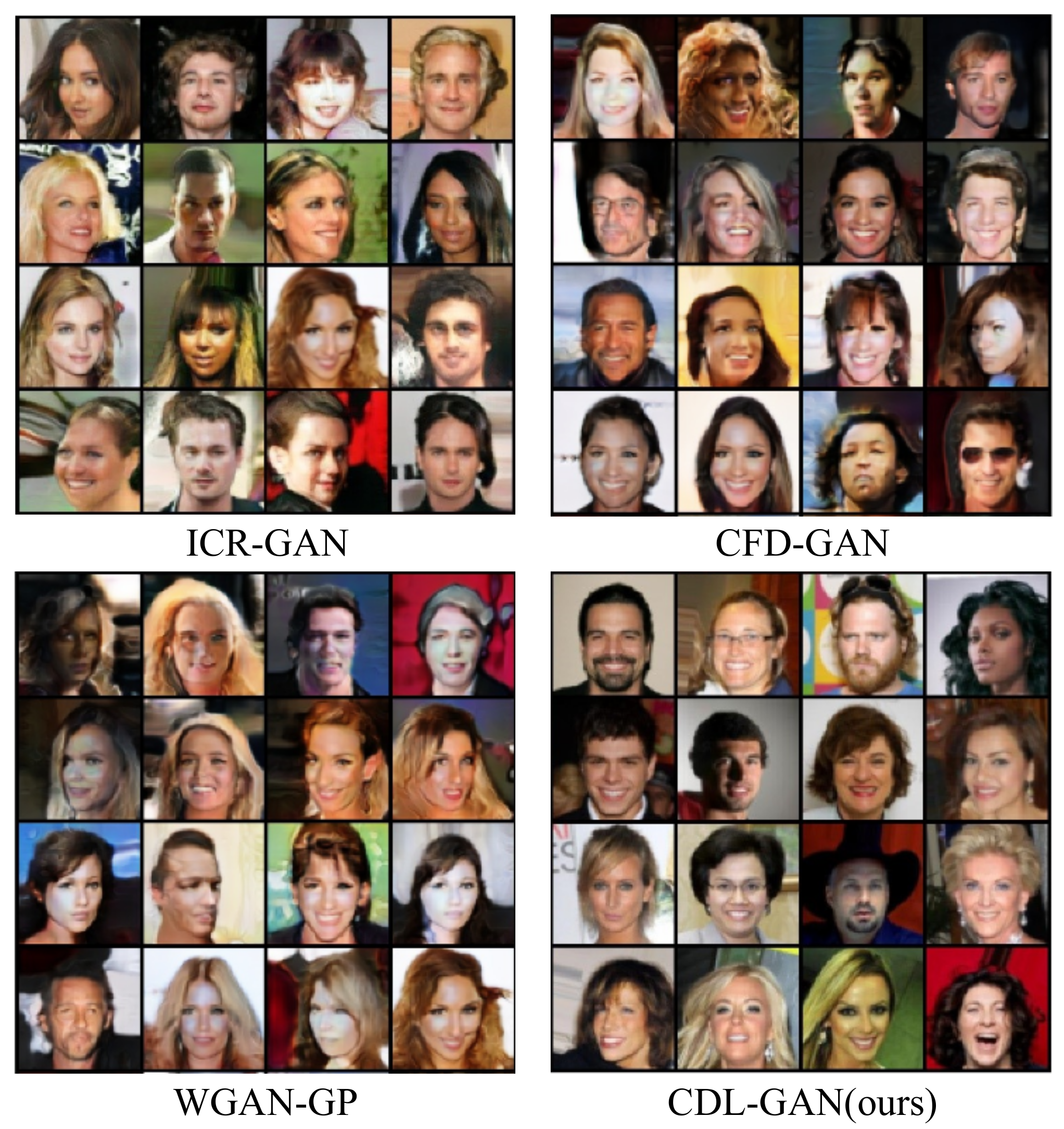
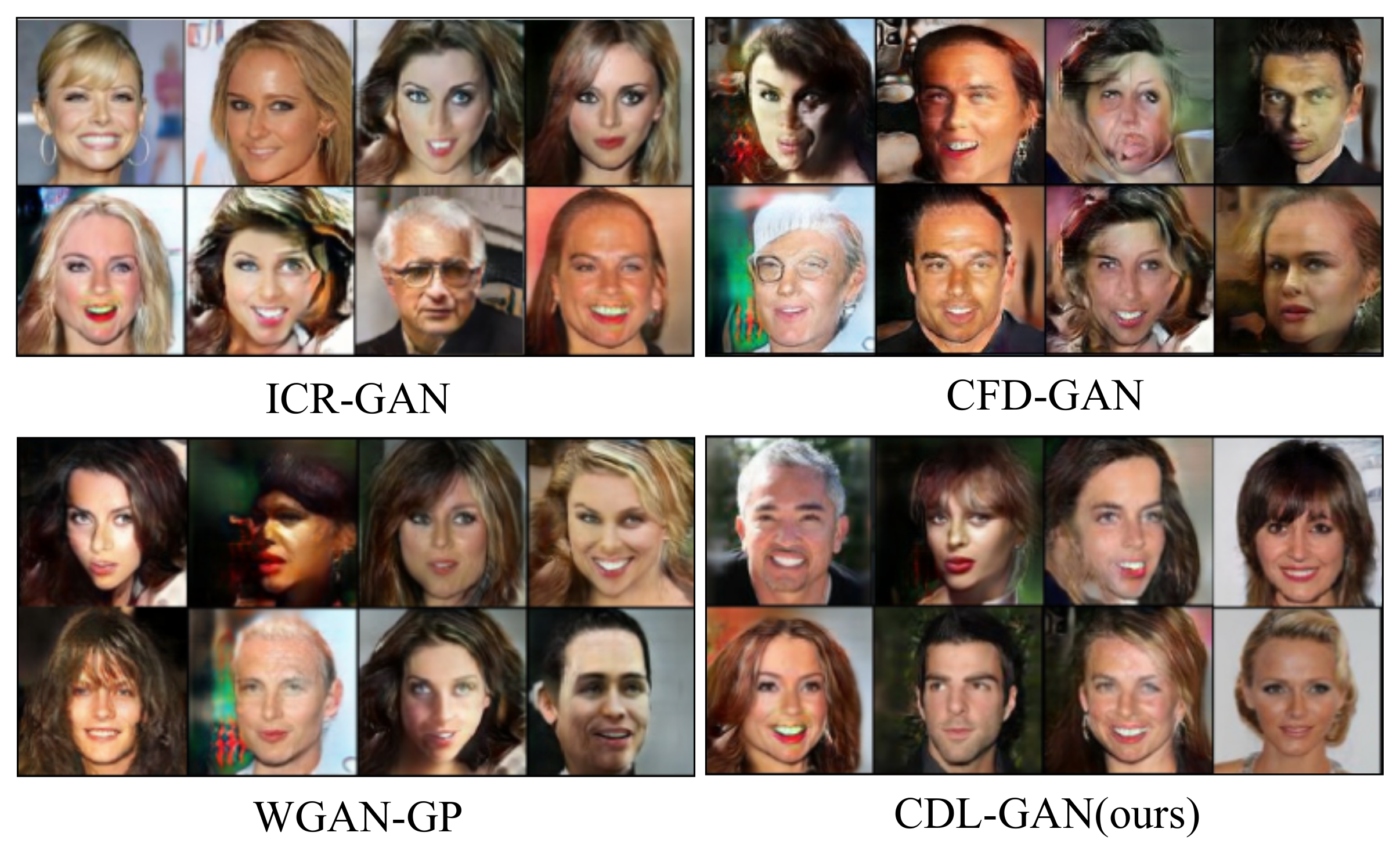
4.2. Results
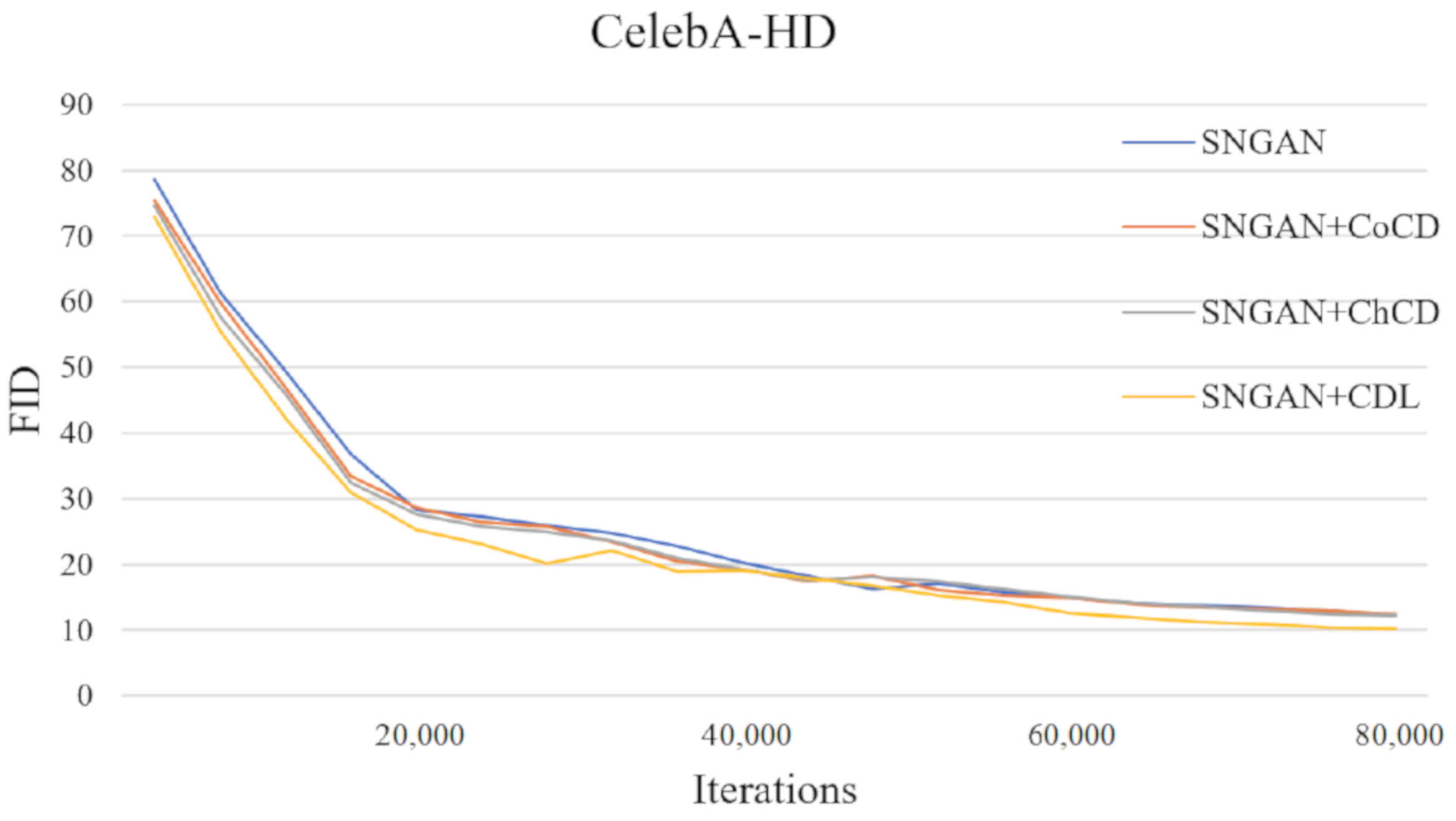
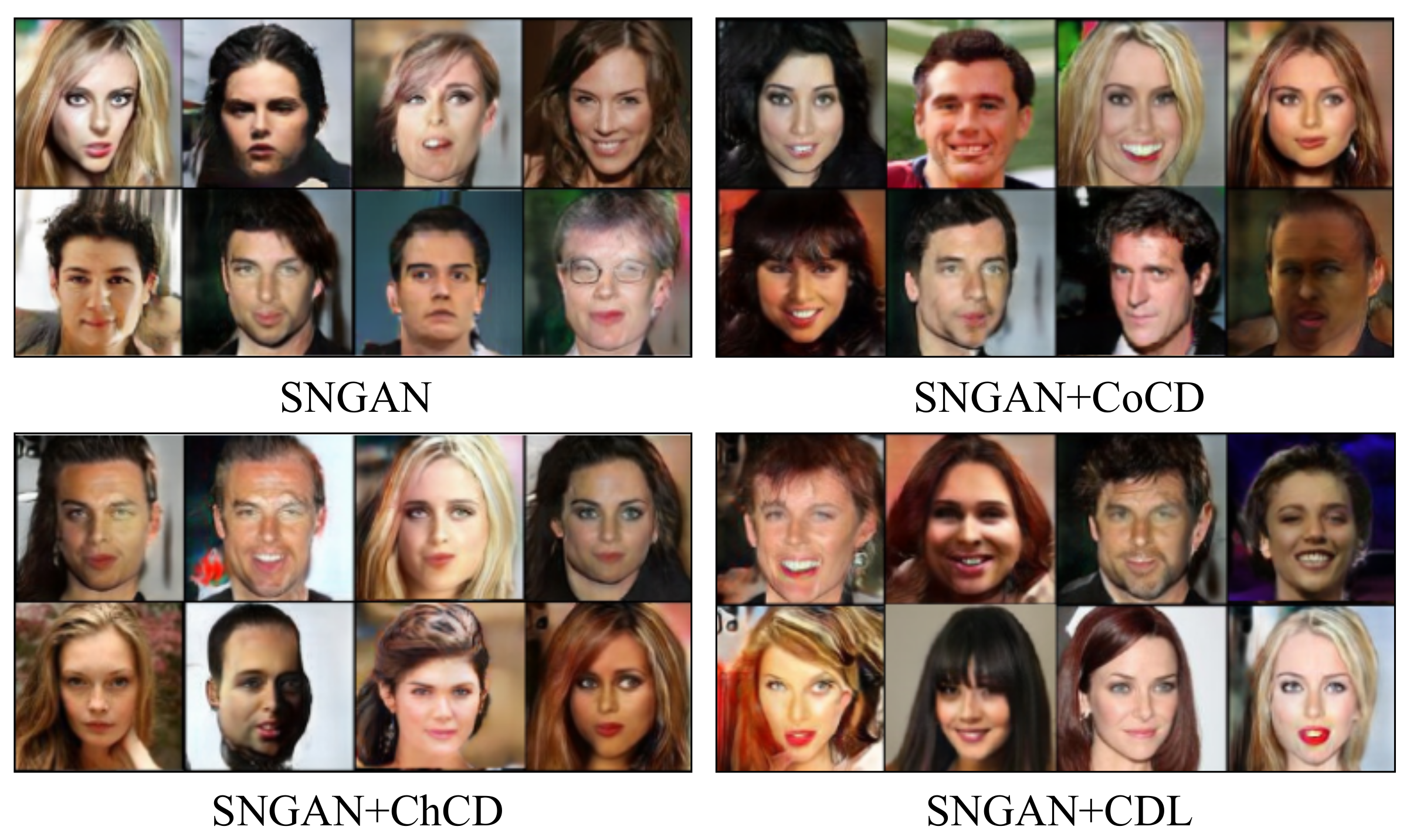
4.3. Ablation Study
5. Conclusions and Discussion
Author Contributions
Funding
Institutional Review Board Statement
Informed Consent Statement
Data Availability Statement
Conflicts of Interest
References
- Goodfellow, I.J.; Pouget-Abadie, J.; Mirza, M.; Bing, X.; Bengio, Y. Generative adversarial nets. In Proceedings of the Advances in Neural Information Processing Systems, Montreal, QC, Canada, 8–13 December 2014; pp. 2672–2680. [Google Scholar]
- Mirza, M.; Osindero, S. Conditional generative adversarial nets. arXiv 2014, arXiv:1411.1784. [Google Scholar]
- Huang, X.; Li, Y.; Poursaeed, O.; Hopcroft, J.; Belongie, S. Stacked generative adversarial networks. In Proceedings of the IEEE Conference on Computer Vision and Pattern Recognition, Honolulu, HI, USA, 21–26 July 2017; pp. 5077–5086. [Google Scholar]
- Odena, A.; Olah, C.; Shlens, J. Conditional image synthesis with auxiliary classifier gans. In Proceedings of the International Conference on Machine Learning, Sydney, Australia, 6–11 August 2017; pp. 2642–2651. [Google Scholar]
- Wang, Y.; Zhang, L.; Van De Weijer, J. Ensembles of generative adversarial networks. arXiv 2016, arXiv:1612.00991. [Google Scholar]
- Hoang, Q.; Nguyen, T.D.; Le, T.; Phung, D. Multi-generator generative adversarial nets. arXiv 2017, arXiv:1708.02556. [Google Scholar]
- Nguyen, T.; Le, T.; Vu, H.; Phung, D. Dual discriminator generative adversarial nets. In Proceedings of the Advances in Neural Information Processing Systems, Long Beach, CA, USA, 4–9 December 2017; pp. 2670–2680. [Google Scholar]
- Larsen, A.B.L.; Sønderby, S.K.; Larochelle, H.; Winther, O. Autoencoding beyond pixels using a learned similarity metric. In Proceedings of the International Conference on Machine Learning, New York, NY, USA, 19–24 June 2016; pp. 1558–1566. [Google Scholar]
- Makhzani, A.; Shlens, J.; Jaitly, N.; Goodfellow, I.; Frey, B. Adversarial autoencoders. arXiv 2015, arXiv:1511.05644. [Google Scholar]
- Dumoulin, V.; Belghazi, I.; Poole, B.; Mastropietro, O.; Lamb, A.; Arjovsky, M.; Courville, A. Adversarially learned inference. arXiv 2016, arXiv:1606.00704. [Google Scholar]
- Wang, X.; Wang, X. Unsupervised Domain Adaptation with Coupled Generative Adversarial Autoencoders. Appl. Sci. 2018, 8, 2529. [Google Scholar] [CrossRef]
- Kwak, J.g.; Ko, H. Unsupervised Generation and Synthesis of Facial Images via an Auto-Encoder-Based Deep Generative Adversarial Network. Appl. Sci. 2020, 10, 1995. [Google Scholar] [CrossRef]
- Arjovsky, M.; Chintala, S.; Bottou, L. Wasserstein gan. arXiv 2017, arXiv:1701.07875. [Google Scholar]
- Miyato, T.; Kataoka, T.; Koyama, M.; Yoshida, Y. Spectral normalization for generative adversarial networks. arXiv 2018, arXiv:1802.05957. [Google Scholar]
- Salimans, T.; Zhang, H.; Radford, A.; Metaxas, D. Improving GANs using optimal transport. arXiv 2018, arXiv:1803.05573. [Google Scholar]
- Li, C.L.; Chang, W.C.; Cheng, Y.; Yang, Y.; Póczos, B. Mmd gan: Towards deeper understanding of moment matching network. In Proceedings of the Advances in Neural Information Processing Systems, Long Beach, CA, USA, 4–9 December 2017; pp. 2203–2213. [Google Scholar]
- DeVries, T.; Taylor, G.W. Improved regularization of convolutional neural networks with cutout. arXiv 2017, arXiv:1708.04552. [Google Scholar]
- Wei, X.; Gong, B.; Liu, Z.; Lu, W.; Wang, L. Improving the improved training of wasserstein gans: A consistency term and its dual effect. arXiv 2018, arXiv:1803.01541. [Google Scholar]
- Odena, A.; Zhang, H.; Lee, H.; Zhang, Z. Consistency Regularization for Generative Adversarial Networks. arXiv 2019, arXiv:1910.12027. [Google Scholar]
- Mao, Q.; Lee, H.Y.; Tseng, H.Y.; Ma, S.; Yang, M.H. Mode seeking generative adversarial networks for diverse image synthesis. In Proceedings of the IEEE Conference on Computer Vision and Pattern Recognition, Long Beach, CA, USA, 16–20 June 2019; pp. 1429–1437. [Google Scholar]
- Zhao, Z.; Singh, S.; Lee, H.; Zhang, Z.; Odena, A.; Zhang, H. Improved consistency regularization for gans. arXiv 2020, arXiv:2002.04724. [Google Scholar]
- Ansari, A.F.; Scarlett, J.; Soh, H. A Characteristic Function Approach to Deep Implicit Generative Modeling. In Proceedings of the IEEE/CVF Conference on Computer Vision and Pattern Recognition, Seattle, WA, USA, 13–19 June 2020; pp. 7478–7487. [Google Scholar]
- Mescheder, L.; Nowozin, S.; Geiger, A. The numerics of gans. In Proceedings of the Advances in Neural Information Processing Systems, Long Beach, CA, USA, 4–9 December 2017; pp. 1825–1835. [Google Scholar]
- Daskalakis, C.; Ilyas, A.; Syrgkanis, V.; Zeng, H. Training gans with optimism. arXiv 2017, arXiv:1711.00141. [Google Scholar]
- Prasad, H.; LA, P.; Bhatnagar, S. Two-timescale algorithms for learning Nash equilibria in general-sum stochastic games. In Proceedings of the 2015 International Conference on Autonomous Agents and Multiagent Systems, Istanbul, Turkey, 4–8 May 2015; pp. 1371–1379. [Google Scholar]
- Yadav, A.; Shah, S.; Xu, Z.; Jacobs, D.; Goldstein, T. Stabilizing adversarial nets with prediction methods. arXiv 2017, arXiv:1705.07364. [Google Scholar]
- Miyato, T.; Koyama, M. cGANs with projection discriminator. arXiv 2018, arXiv:1802.05637. [Google Scholar]
- Heusel, M.; Ramsauer, H.; Unterthiner, T.; Nessler, B.; Hochreiter, S. Gans trained by a two time-scale update rule converge to a local nash equilibrium. In Proceedings of the Advances in Neural Information Processing Systems, Long Beach, CA, USA, 4–9 December 2017; pp. 6626–6637. [Google Scholar]
- Lim, J.H.; Ye, J.C. Geometric gan. arXiv 2017, arXiv:1705.02894. [Google Scholar]
- Villani, C. Optimal Transport: Old and New; Springer Science & Business Media: Berlin/Heidelberg, Germany, 2008; Volume 338. [Google Scholar]
- Gulrajani, I.; Ahmed, F.; Arjovsky, M.; Dumoulin, V.; Courville, A.C. Improved training of wasserstein gans. In Proceedings of the Advances in Neural Information Processing Systems, Long Beach, CA, USA, 4–9 December 2017; pp. 5767–5777. [Google Scholar]
- Miyato, T.; Maeda, S.i.; Koyama, M.; Ishii, S. Virtual adversarial training: A regularization method for supervised and semi-supervised learning. IEEE Trans. Pattern Anal. Mach. Intell. 2018, 41, 1979–1993. [Google Scholar] [CrossRef]
- Chwialkowski, K.P.; Ramdas, A.; Sejdinovic, D.; Gretton, A. Fast two-sample testing with analytic representations of probability measures. In Proceedings of the Advances in Neural Information Processing Systems, Montreal, QC, Canada, 7–12 December 2015; pp. 1981–1989. [Google Scholar]
- Epps, T.; Singleton, K.J. An omnibus test for the two-sample problem using the empirical characteristic function. J. Stat. Comput. Simul. 1986, 26, 177–203. [Google Scholar] [CrossRef]
- Heathcote, C. A test of goodness of fit for symmetric random variables1. Aust. J. Stat. 1972, 14, 172–181. [Google Scholar] [CrossRef]
- Bromley, J.; Guyon, I.; Lecun, Y.; Sckinger, E.; Shah, R. Signature Verification Using a Siamese Time Delay Neural Network. In Proceedings of the Advances in Neural Information Processing Systems 6, 7th NIPS Conference, Denver, CO, USA, 22–23 November 1993. [Google Scholar]
- Nair, V.; Hinton, G.E. Rectified linear units improve restricted boltzmann machines. In Proceedings of the 27th International Conference on Machine Learning, Haifa, Israel, 21–24 June 2010. [Google Scholar]
- Bertinetto, L.; Valmadre, J.; Henriques, J.F.; Vedaldi, A.; Torr, P.H.S. Fully-Convolutional Siamese Networks for Object Tracking. In Proceedings of the Computer Vision—ECCV 2016 Workshops, Amsterdam, The Netherlands, 8–10, 15–16 October 2016; pp. 850–865. [Google Scholar]
- Xu, Z.; Luo, H.; Hui, B.; Chang, Z.; Ju, M. Siamese Tracking with Adaptive Template-Updating Strategy. Appl. Sci. 2019, 9, 3725. [Google Scholar] [CrossRef]
- Amodio, M.; Krishnaswamy, S. Travelgan: Image-to-image translation by transformation vector learning. In Proceedings of the IEEE Conference on Computer Vision and Pattern Recognition, Long Beach, CA, USA, 16–20 June 2019; pp. 8983–8992. [Google Scholar]
- Zagoruyko, S.; Komodakis, N. Learning to compare image patches via convolutional neural networks. In Proceedings of the IEEE Conference on Computer Vision and Pattern Recognition, Boston, MA, USA, 7–12 June 2015; pp. 4353–4361. [Google Scholar]
- Da, K. A method for stochastic optimization. arXiv 2014, arXiv:1412.6980. [Google Scholar]
- Radford, A.; Metz, L.; Chintala, S. Unsupervised representation learning with deep convolutional generative adversarial networks. arXiv 2015, arXiv:1511.06434. [Google Scholar]
- LeCun, Y.; Bottou, L.; Bengio, Y.; Haffner, P. Gradient-based learning applied to document recognition. Proc. IEEE 1998, 86, 2278–2324. [Google Scholar] [CrossRef]
- Krizhevsky, A.; Hinton, G. Learning multiple layers of features from tiny images. In Handbook of Systemic Autoimmune Diseases; Elsevier: Amsterdam, The Netherlands, 2009. [Google Scholar]
- Liu, Z.; Luo, P.; Wang, X.; Tang, X. Deep Learning Face Attributes in the Wild. In Proceedings of the IEEE International Conference on Computer Vision (ICCV), Santiago, Chile, 7–13 December 2015. [Google Scholar]
- Kurach, K.; Lucic, M.; Zhai, X.; Michalski, M.; Gelly, S. A Large-Scale Study on Regularization and Normalization in GANs. arXiv 2019, arXiv:1807.04720. [Google Scholar]
- Metz, L.; Poole, B.; Pfau, D.; Sohl-Dickstein, J. Unrolled Generative Adversarial Networks. arXiv 2016, arXiv:1611.02163. [Google Scholar]


| Models | MNIST (32*32) | CIFAR-10 (32*32) | CelebA (64*64) | CelebA-HD (128*128) |
|---|---|---|---|---|
| ICR-GAN | 0.55 | 15.87 | 15.43 | 19.56 |
| CFD-GAN | 0.53 | 33.08 | 20.48 | 25.73 |
| WGAN-GP | 0.69 | 22.29 | 17.85 | 23.98 |
| CDL-GAN (ours) | 0.48 | 14.33 | 13.18 | 16.53 |
| SNGAN | SNGAN + CoCD | SNGAN + ChCD | SNGAN + CDL | |
|---|---|---|---|---|
| (0.0, 0.9) | 12.97 | 12.12 | 11.35 | 10.08 |
| (0.5, 0.999) | 14.88 | 13.33 | 12.98 | 10.27 |
| Metric | K | DCGAN | ICR-GAN | CDL-GAN |
|---|---|---|---|---|
| Modes | 30.64 | 48.47 | 50.50 | |
| Modes | 605.17 | 703.25 | 725.88 | |
| 5.48 | 4.96 | 4.55 | ||
| 1.97 | 1.64 | 1.45 |
Publisher’s Note: MDPI stays neutral with regard to jurisdictional claims in published maps and institutional affiliations. |
© 2021 by the authors. Licensee MDPI, Basel, Switzerland. This article is an open access article distributed under the terms and conditions of the Creative Commons Attribution (CC BY) license (http://creativecommons.org/licenses/by/4.0/).
Share and Cite
Zhou, Y.; Zhao, P.; Tong, W.; Zhu, Y. CDL-GAN: Contrastive Distance Learning Generative Adversarial Network for Image Generation. Appl. Sci. 2021, 11, 1380. https://doi.org/10.3390/app11041380
Zhou Y, Zhao P, Tong W, Zhu Y. CDL-GAN: Contrastive Distance Learning Generative Adversarial Network for Image Generation. Applied Sciences. 2021; 11(4):1380. https://doi.org/10.3390/app11041380
Chicago/Turabian StyleZhou, Yingbo, Pengcheng Zhao, Weiqin Tong, and Yongxin Zhu. 2021. "CDL-GAN: Contrastive Distance Learning Generative Adversarial Network for Image Generation" Applied Sciences 11, no. 4: 1380. https://doi.org/10.3390/app11041380
APA StyleZhou, Y., Zhao, P., Tong, W., & Zhu, Y. (2021). CDL-GAN: Contrastive Distance Learning Generative Adversarial Network for Image Generation. Applied Sciences, 11(4), 1380. https://doi.org/10.3390/app11041380