Article

Electrical Conductivity Evidence for the Existence of a Mantle Plume Beneath Tarim Basin

College of Geo-exploration Science and Technology, Jilin University, Changchun 130000, China
*
Author to whom correspondence should be addressed.
Appl. Sci. 2021, 11(3), 893; https://doi.org/10.3390/app11030893
Submission received: 25 November 2020 / Revised: 12 January 2021 / Accepted: 18 January 2021 / Published: 20 January 2021
(This article belongs to the Section Earth Sciences)

Abstract

:
This paper proposes using a simulated annealing (SA) calculation to perform one-dimensional inversion of Geomagnetic Depth Sounding (GDS) to obtain the conductivity information of the lower mantle beneath the Tarim area, to calculate the temperature of the lower mantle according to the relevant formula of the petrophysical experiment, and to provide evidence of the existence of the Tarim mantle plume. The data used for inversion originate from the China Geomagnetic Network Center. This article uses theoretical data to prove that the simulated annealing algorithm can invert the true conductivity model when the data do not contain noise. However, when the data contain noise, it is more accurate to use the statistical expected value of the high-quality conductivity model during the simulated annealing inversion process as the optimal conductivity model rather than the classic simulated annealing algorithm. The simulated annealing inversion results of only four stations in Tarim area show that the conductivity of the top of the lower mantle and the upper part of the mantle transition zone in Tarim area is higher than the global average, and it is speculated that the temperature is 150k–450k higher than the global average. This is important evidence for the existence of the mantle plume beneath the Tarim Basin.

1. Introduction

The Tarim Basin is located in the western part of China. Since 50~60 Ma, the India/Asia collision has resulted in strong uplift, shortening, and strike slip deformation around the Tarim Basin, resulting in the formation of a complex ringed mountain system [1]. The movement of the deep mantle is one of the important factors affecting the activity of the top crust. In a large number of seismic profiles, it is found that there is a large-scale transverse low velocity anomaly beneath the Tarim Basin [2,3]. Kosarev pointed out that this may indicate the existence of a mantle plume [4].
A mantle plume, first proposed by Morgan [5,6], is a columnar body produced in the thermal boundary layer of the mantle, driven by buoyancy anomalies and upwelling of deep mantle material [7,8]. Campbell believes that the mantle plume originated from the core-mantle boundary at 2900 km or the seismic discontinuity at about 660 km [9]. The diameter of the mantle plume can be up to hundreds of kilometers, and it has an abnormally high temperature. This localized high temperature anomaly can cause a dramatic increase in electrical conductivity in the transition zone and the lower mantle. Therefore, this renders us an opportunity to use the geomagnetic depth sounding (GDS) method to explore the possible existence of the mantle plume by studying the conductivity model of the mantle transition zone beneath Northwest China [10].
The electrical conductivity of the deep part of the earth, especially in the range of 410~1600 km, can be effectively reflected by the variation with periods of the C-response of GDS [11]. This parameter is estimated from the horizontal and vertical magnetic field data recorded by geomagnetic stations [12,13]. The intensity of the induced magnetic field is affected by the conductive convective fluid in the core and the mantle, crust, ionosphere, magnetosphere, and ocean current systems and changes over time [14,15]. Therefore, by investigating the changes in the intensity of the surface magnetic field, the internal conductivity of the earth at different depths can be obtained, from which the physical and chemical characteristics and the dynamic mechanisms in Earth’s interior can be resolved [16,17].
Inversion is the key to convert C-responses to electrical conductivity profiles. For instance, Munch et al. used stochastic optimization and model exploration techniques to perform one-dimensional inversion of geomagnetic depth sounding, and combined with experimental data of temperature, pressure, and the water content, they obtained temperature information of the mantle transition zone in Europe and Africa [18]. Zhang et al. carried out a one-dimensional inversion of the smooth model based on the geomagnetic data obtained by the global smoothing constraint technique and obtained the water content distribution of the mantle transition zone in eastern China [19]. These one-dimensional inversion results perfectly show the conductivity characteristics of the deep part of the earth, and can provide estimations of temperature and the water content in transition zones. However, these study areas are far from Tarim area. The global GDS inversion may reflect the conductivity characteristics beneath Tarim area, for example, using the three-dimensional nonlinear conjugate gradient method, the first electrical conductivity image of mantle transition zone was obtained by Kelbert et al. [20], but they focused the high conductivity structure of the mantle beneath NE China, while Semenov et al. paid more attention to the electrical conductivity in the transition zone beneath Europe and Africa by using the limited memory quasi-Newton method [21,22]. Nonetheless, due to the sparse data set used, the resolution of the electrical structure beneath Tarim area is very low.
In this paper, we try to invert the GDS response in Tarim area by the non-heuristic algorithm of simulated annealing (SA) to provide a new reference for studying the deep electrical conductivity structure beneath the Tarim area. Similar to the genetic algorithm and artificial neural network [23,24,25], SA is a global optimization method that has been applied with good effect to geophysical inversion [26,27,28]. Traditional SA inversion accepts the model of the last iteration as the inversion result. However, this resultant model can vary significantly due to the nature of random inversion techniques, such as SA. Therefore, here we will conduct the statistical analysis of all effective random inversion models, and use the statistical model as the one-dimensional random inversion result of GDS data. To this end, the paper first briefly introduces the basic process of obtaining the C-response of geomagnetic depth sounding; then, the article addresses the stochastic inversion technique. After that, the above technique is applied to invert the GDS data from four geomagnetic stations (Wushi (WUS), Urumqi (WMQ), HongQian (HOQ), and WenQuan (WEQ)) in Northwest China to obtain the conductivities in and below transition zone. Finally, the model robustness followed by the model interpretation with abnormal temperature beneath Tarim area is discussed. Our research results can provide a very important scientific basis for the study of the evolutionary process of the orogenic belt around the Tarim Basin. From the perspective of Geophysics, we can see that there may be a high temperature mantle plume in the lower part of the Tarim Basin (this mantle plume has little to do with the Tarim large igneous province).

2. Materials and Methods

2.1. Data

We collected the data from the four stations in Northwest China from the China Geomagnetic Network Center (Figure 1). The data information is listed in Table 1. These geomagnetic stations have just been established; the data have not yet been explored. The application of the new data will provide new insights into the deep structure of the earth.
In order to make better use of these data, it is necessary to use approximate methods to estimate the C-response, which can be written in the following form
C = a 0 tan θ 2 H r H θ .
In the formula, tanθ is regarded as the compensation term of the source space. a0 is the radius of the earth and its value is 6370 km. In the study of geomagnetic depth sounding (GDS), a spherical coordinate system whose origin is defined at the center of the earth is used. Among them, Hr points to the center of the earth, Hθ is the tangential component of the magnetic field, and θ is the geomagnetic colatitude. C-response establishes the relationship between surface observation data and the internal electrical structure of the earth [29,30].
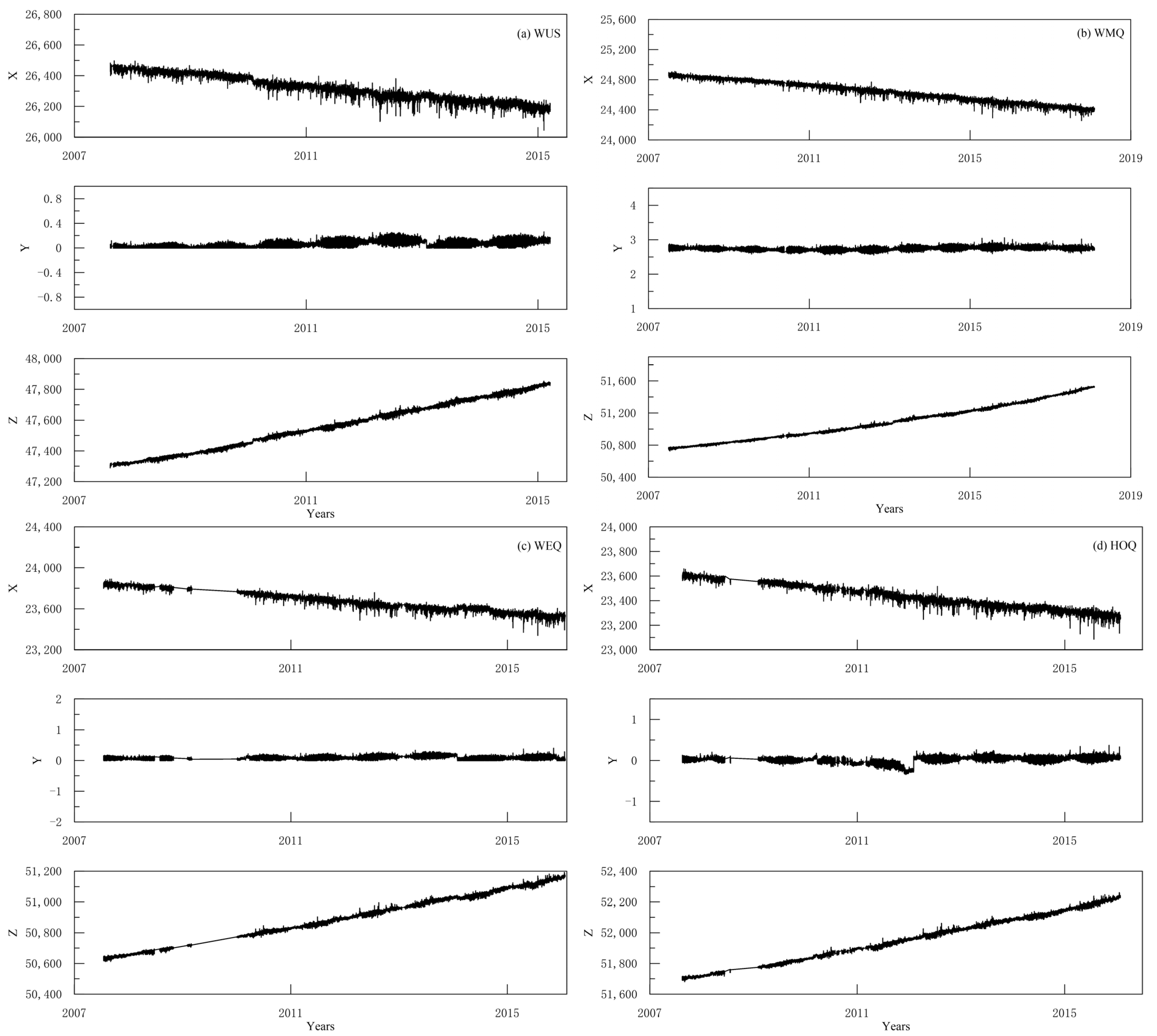
All four geomagnetic stations record the changes of the geomagnetic component at the time. Figure 2 shows the long and continuous signals recorded by the four geomagnetic stations.
In addition, the data record length for these stations is continuous and sufficiently long, so that there are enough time segments that can be superimposed in the Fourier transform of each period, and the data error can be well suppressed to obtain a stable C-response in the period from several days to hundreds of days. If the observation times of the station were longer than five years, the geomagnetic data of continuous records could be used to invert conductivity in the mantle transition zone [31].
When estimating C-responses, the long-term field should be removed from the high-quality time series. This is because the GDS only includes the magnetic field generated by the magnetospheric current source on the earth’s surface, while the long-term changing fields as the main component in the geomagnetic field observed by geomagnetic stations are generated inside the earth. Long-term fields can be calculated using the code provided by the International Association of Geomagnetism and Aeronomy (https://www.ngdc.noaa.gov/IAGA/vmod/igrf12) [32]. After that, the horizontal component of the geomagnetic field also needs to be converted from the geographic coordinate system to the geomagnetic (dipole) coordinate system. Finally, the obtained time series is processed with Bounded Influence Remote Reference Processing BIRRP software to estimate the frequency spectrum of Hr and Hθ corresponding to the estimated C-response according to Equation (1) and the coherence square coh2 of each frequency, from which the data error can be estimated through the equation as
δ C = | C | 1 coh 2 coh 2 ( 1 β ) 1 z 1 .
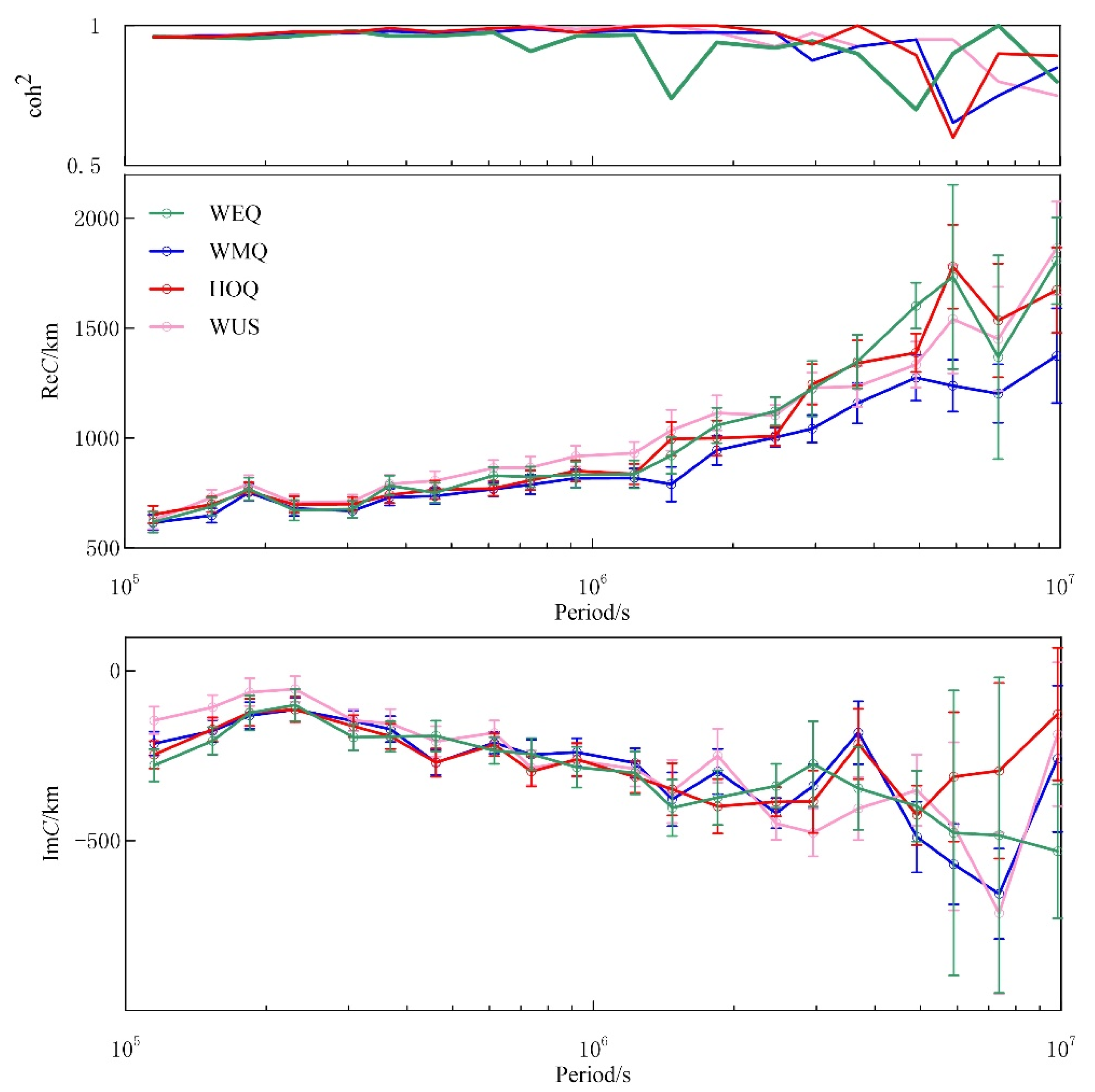
where coh2 is the squared coherence which can be used to assess the quality of the estimated C-responses. 1/β is the confidence level and is often set as 0.9; Z is the number of sections for a certain frequency. BIRRP is data processing software for geomagnetic sounding and the magnetotelluric response function proposed by Chave and Thomson [33]. The C-responses and squared coherence coefficients of the four stations finally obtained are shown in Figure 3. It can be seen that the C-responses at the four stations possess the same characteristics. In the short periods, the C-responses from different stations almost overlap each other, signifying that our C-responses are reliable. The errors indicated by the error bars in the short periods are rather low; in long periods, the error bars become wide, but are in the acceptable range. All these imply that our C-responses are overall of good quality.

2.2. Inversion Algorithm

2.2.1. SA Inversion

One-dimensional inversion of GDS can be achieved by minimizing the following objective function:
E ^ ( σ , ω , λ ) = N ω [ lg | C obs ( ω ) | lg | C mod ( ω ) | ] 2 + λ f m ( σ ) ,
where λ is the regularization factor; Nω is the number of frequencies; Cobs(ω) is the C-response computed from the observed data; and Cmod(ω) is the model theoretical C-response. fm is the model constraint describing the smoothness of the model. σ is the conductivity model vector and is the parameter that needs to be inverted. In this case, the thicknesses of the thin spheres that make up the Earth are fixed and do not participate in the inversion. The process of minimizing the objective functional is similar to the process of cooling a high-energy solid material to reach a steady state of minimal energy [34]. Thus, the simulated annealing nonlinear optimization algorithm can be adapted for the one-dimensional GDS inversion. In this case, the objective function defined by Equation (3) is taken as the energy function in the annealing process. By reducing the temperature in an appropriate manner, the state corresponding to each molecule when the value of the objective function reaches the minimuml can be accepted as the solution of an inversion problem.
The improved simulated annealing (ISA) algorithm proposed in this paper is based on traditional simulated annealing combined with statistical analysis to improve the robustness of inversion. The main steps in the flowchart include:
  • Initialization: T0, M, σmax, σmin, σ0, L, RMSmax, i = 0.
  • Set l = 1 and perform a Markov chain loop L times.
    2.1
    Generate a model σil randomly; calculate its corresponding objective function value and RMS;
    2.2
    When RMS is less than RMSmax, save the model as a member of the solution set for statistical analysis in step 5;
    2.3
    When the objective function value E ^ corresponding to the model σil meets the Metropolis criterion, the model is used as the current optimal solution. The loop continues if the value E ^ corresponding to the model does not meet the Metropolis criterion;
    2.4
    Update l: l = l + 1;
  • Decrease temperature T; i = i +1.
  • When i > M, the annealing cycle ends; otherwise, return to step 2.
  • Statistical calculation of the optimal solution: Perform statistical analysis on all models with RMS less than RMSmax to determine the final solution.
In the above iteration process, T0 is the initial temperature; i is the current number of iterations; M is the upper limit of the number of iterations; l is the current number of cycles in the chain, which is controlled by the chain length L of the Markov chain. When the value of L increases, the number of global searches at the same temperature increases, and as a result, there is a greater probability of obtaining the global optimal solution [35]. Considering the time cost, after our experimental verifications, L = 10 can achieve the search purpose. σmax and σmin are the conductivity value boundaries, and they can be estimated based on known petrophysical models or previous experience [36]. σ0 is the initial value of the model. SA inversion does not require a fixed initial model, so the initial value is a random number within the valid range.
RMSmax represents the threshold of RMS, while RMS here is defined by
R M S = 1 N ω i = 1 N ω ( C mod ( ω ) C o b s ( ω ) C o b s ( ω ) ) 2 .
An appropriate choice of RMSmax is essential for inversion [25]. The selection of a reasonable RMSmax needs to consider factors such as the data quality of the C-response and the number of iterations. The basic principle of RMSmax setting is to require the threshold to filter out a large enough sample size in accordance with the log-normal distribution during the inversion process, otherwise the RMSmax needs to be adjusted during the inversion process.
It is worth noting that in the above steps, the optimal solution obtained by the traditional SA algorithm is the final iteration result in steps (1)–(4). When step (5) is added, the inversion result is no longer a simple choice based on the result of the last iteration, but is determined by the statistical expected value of all the solutions that meet the constraint conditions during the SA inversion. Therefore, this model can better reflect the characteristics of random inversion while retaining the minimal energy state.

2.2.2. Random Model Generator

The random conductivity parameters conform to the temperature-related Cauchy distribution, and the specific formula is as follows:
σ i k + 1 = σ i k + y i ( σ i max σ i min ) ,
y i = sgn ( u i 0.5 ) T k { ( 1 + 1 / T k ) | 2 u i 1 | 1 } .
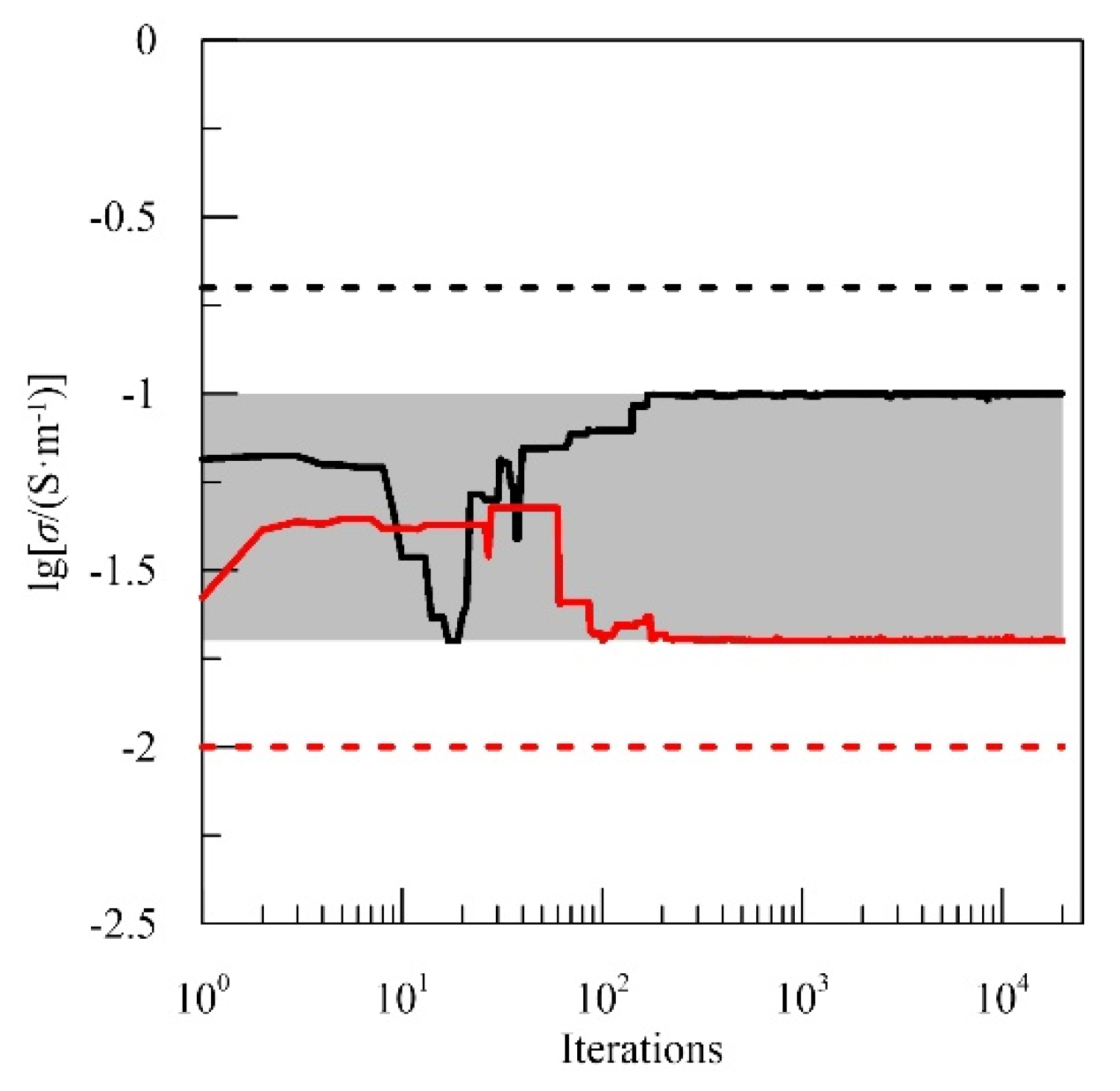
In above equations, yi is the updated factor of the i-th (i = 1, 2, …, N) parameter, yi ∈ [−1, 1]; Tk is the temperature corresponding to the k-th iteration. ui is a uniformly distributed random variable between 0 and 1, and sgn represents a sign function. The selected and inverted results are constrained by the range of model parameters. As a result, if the model parameter interval was selected unreasonably, for example, to be in a narrower range, the inversion results would then be concentrated at the interval boundary (Figure 4). At this time, the upper and lower limits of the parameter interval should be appropriately expanded [37,38].

2.2.3. Metropolis Criterion

Whether the currently randomly modified model is accepted or not needs to be judged according to Metropolis guidelines. The criterion needs to calculate the acceptance probability P of the new state by
P = exp ( Δ E ^ / T k ) ,
where
Δ E ^ = E ^ ( σ k + 1 ) E ^ ( σ k )
represents the difference in the objective function (energy) between the modified model and the current optimal model. If Δ E ^ < 0 , the current solution is better than the historical optimal solution, P = 100% is agreed, and the model is fully accepted as the optimal solution in the iteration process for the next iteration. Otherwise, it means that the current solution is inferior to the historical optimal solution, and the probability P is calculated according to Formula (7) and is compared with it with a randomly generated random number uniformly distributed between 0 and 1. When the random number is less than P, the model is accepted. When the random number is greater than P, the model is not accepted and the cycle continues. The Metropolis criterion makes it possible for the solution to escape the local minimum.

2.2.4. Decreasing Temperature

A reasonable annealing temperature reduction mechanism can efficiently control the convergence of the iterative process to obtain an approximate optimal solution. The formula for controlling the decrease of the temperature T at the k-th iteration during the inversion process is
T ( k ) = T 0 exp ( c k 1 / m ) .
Here, c is a constant. T0 is the initial temperature. A high initial temperature will cause the solution to converge slowly at the beginning of the iteration, so it is not necessary to choose a high initial temperature. According to Sharma, in the DC bathymetry inversion experiment, the value of c was set to 1, the value of T0 was set to 0.01, and the value of m was set to 2.5, which can ensure the efficiency of the inversion, and they do not depend on the model parameters during the inversion process [39]. Through experiments, we have verified that this set of parameters is also more applicable to geomagnetic depth sounding.

2.3. Statistical Analysis of the Solution Distribution

Since the conductivity parameter cannot be a negative value, all the effective model parameters in the iterative process could be described by a lognormal distribution, and lnσ obeys a normal distribution with expectation μ and variance ε2. For a certain layer, the final conductivity value of the inversion is equal to the expected value E(σ) of the effective conductivity parameter set of the layer, and the estimation formula is
E ( σ ) = e μ + ε 2 / 2 ,
where ε is the standard deviation that can measure the uncertainty of the result. When ε is smaller, the estimated value is more reliable. The data contained within one standard deviation of the expected value account for 68% of the total data. Therefore, in this article we take this range as the reliability interval.
In order to visualize the reliability of whether the samples of a conductivity parameter obey a lognormal distribution, the P-P lognormal probability diagram is a useful tool. This diagram can determine whether the sample data conform to the lognormal distribution. The P-P diagram is drawn based on the cumulative probability of the variable corresponding to the cumulative probability of the natural log-normal theoretical distribution [39]. The abscissa represents the cumulative probability density of the conductivity sample; the ordinate is the theoretical cumulative probability density, which is calculated by the probability density function
p ( σ ) = 1 σ ε 2 π e ( ln σ μ ) 2 2 ε 2 .
When the used data obey the log-normal distribution, the cumulative probability of the sample is approximately equal to the theoretical cumulative probability, and in the P-P diagram, it will present as a 45° straight line (Figure 5). It can be seen that the sample distribution of the inverted conductivity σ4 basically obeys the log-normal distribution. In the inset, the P-P diagram of the conductivity σ4 of the fourth layer reflects this characteristic.

3. Results

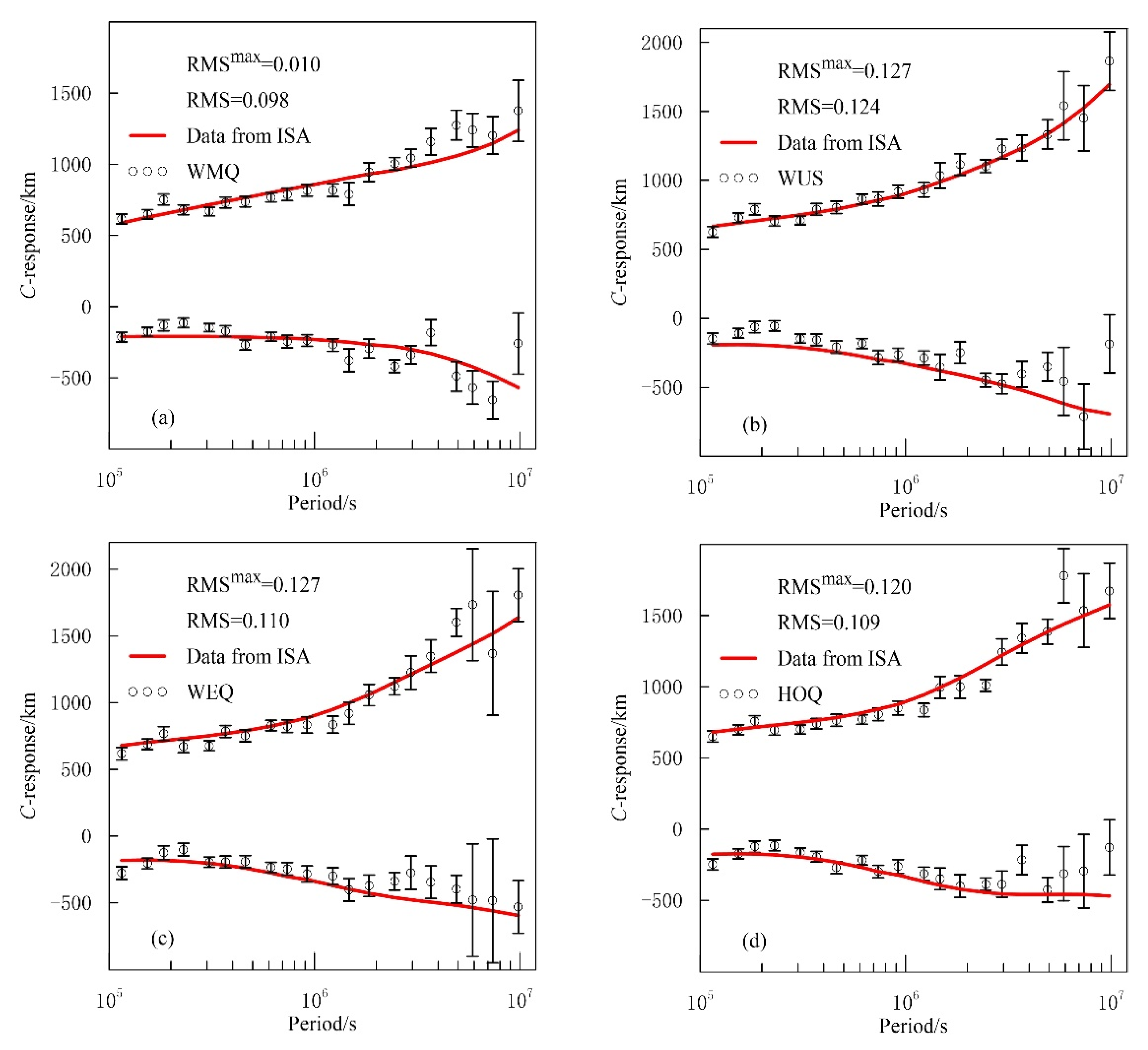
We apply the ISA method to the one-dimensional inversion of measured geomagnetic depth sounding data from four stations around the Tarim area [40]. The above-mentioned stations are located inland at low latitudes. Therefore, their C-responses should not be affected by aurora and ocean effects [41] and thus can be directly inverted [32]. During the inversion, according to the law that the conductivity of the deep mantle jumps with the phase transition of the main minerals [42], nine layers above the core are divided [20]. The possible range for the conductivity of each layer is estimated based on the results of the Semenov inversion [22]. The control parameters of simulated annealing inversion are as follows: M = 3000; L = 10; T0 = 0.01. The control parameter RMSmax is given in Figure 6. The variation range of the conductivity parameter is indicated by the shading in Figure 7. The final ISA inversion results in a smooth C-response curve with the same variation trend as the original data. At the same time, the RMS value is given in the Figure.
Figure 7 shows the final conductivity model beneath Tarim area. Above 410 km, the conductivity values below the four stations are similar. Within the sensitive depth range of geomagnetic depth sounding, there is no obvious conductivity jump under the HOQ and WEQ stations on the 410 km discontinuity, which is consistent with the conductivity characteristics of the continental transition zone obtained by Yoshino [43]. On the same discontinuity surface, the conductivity values below WUS and WMQ stations have greatly increased. We speculate that the transition zone is affected by the mantle plume beneath Tarim. From 520~660 km, the conductivity below the WMQ station in the lower layer of the transition zone is much higher than at the other three stations. At 660~900 km, compared with the lower layer of the transition zone, the conductivity of the top of the lower mantle below the four stations is significantly increased and the value is at the same order of magnitude. The noise test of the theoretical data shows that when the data contain noise, the true value of the conductivity is included in the reliable interval of the conductivity obtained by the inversion. Therefore, we believe that the inversion result of this paper is reasonable.

4. Discussion

4.1. Robustness of ISA Inversion

4.1.1. Model and Synthetic Data

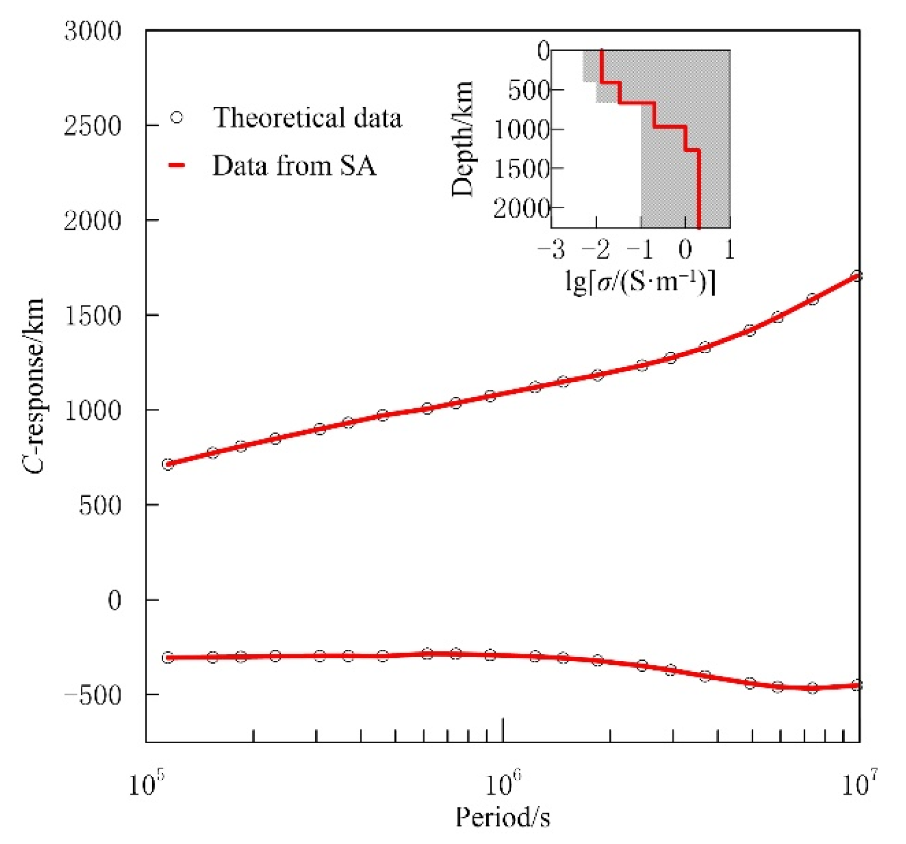
In order to verify the feasibility and correctness of the application of simulated annealing in the one-dimensional inversion of geomagnetic depth sounding, the synthetic model was tested and the results were discussed. The theoretical model is based on Kelbert’s one-dimensional model in the inset of Figure 8 [20], and its theoretical C-response (Figure 8) is inverted as observation data. The model change range during the inversion process is determined according to the maximum change interval of 400 independent one-dimensional global average models obtained by Püthe using the Monte Carlo sampling method [44].

4.1.2. Experimental Results

We first perform an inversion test on the theoretical data without noise, shown in Figure 8. In the simulated annealing inversion process, M is set to 10,000, L is 1, and other parameters are the same as those of Sharma [38]. Figure 9 shows the poor fit and the change of model conductivity during the inversion process and the conductivity values of each layer at the end of the iteration. It can be seen that the RMS has a decreasing trend during the inversion process; since the theoretical C-response value does not contain noise and is accurate enough, according to the RMS calculation formula, its value can be reduced to a value close to zero. When the number of iterations exceeds 3000, the changes in the electrical conductivity of each layer are concentrated near the theoretical true value; when the iteration is greater than 5000, the electrical conductivity of each layer obtained by the inversion has very little difference from the true value. However, there are still cases where the poor model is accepted and the RMS is increased when using Metropolis criteria to judge the results.
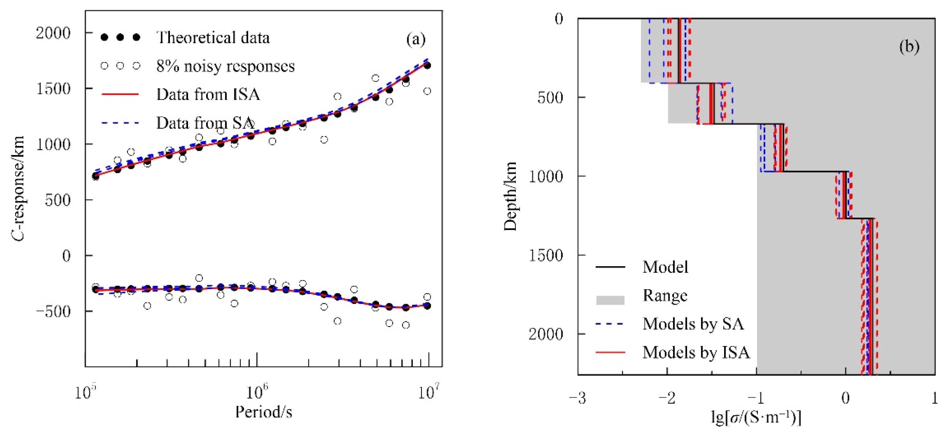
Noise is widespread in actual geomagnetic data [19]. It is generally believed that the C-response affected by excessive noise cannot be used for inversion studies. Therefore, we added an acceptable 8% Gaussian noise to the theoretical C-response in Figure 8 for the inversion method test. Under the same initial conditions as the noise-free data inversion test, the inversion was performed three times using the SA algorithm. It can be seen from Figure 10a that at the end of the inversion, the C-response fitting effect of the three inversions is basically the same. However, it can be seen in Figure 10b that due to the influence of noise, the final solution (three blue dotted lines) obtained by the traditional SA method inversion is quite different. For example, the three results of σ3 are −0.787, −0.952, −0.911 S/m. The three results are quite different from the theoretical conductivity of −0.699 S/m. It is concluded that the inversion results are affected by the difference in the sensitivity of the geomagnetic depth sounding method itself at different depths. It shows that even if the inversion is affected by noise and other factors, and even if the global inversion method is adopted, when the number of iterations is not enough, it is not easy to determine the most reasonable model.
Figure 10 shows that when the traditional SA algorithm is used for inversion, only the last iteration value is taken as the model result, which obviously ignores the distribution characteristics of the conductivity parameters during the iteration process. Therefore, if combined with statistical analysis methods, the estimated value of model conductivity may be calculated more accurately. After that, we use the method of analyzing the distribution characteristics of the solution in Section 2.3 to perform three inversions of the noise-added C-response, and the resulting model after statistical analysis is shown by the (three) red lines in Figure 10b. The initial conditions of the inversion are the same as those in Section 3. The red dotted line represents the upper and lower limits of the estimated value, which can be used as a reliable interval.
Figure 10a,b shows that although the results obtained by the traditional SA method are quite different, the results of ISA are not affected by randomness, and the statistically estimated solutions are basically the same, reflecting the direction of solution convergence. The red lines in the figure basically overlap. Therefore, ISA inversion has stronger stability and accuracy, and it has weaker multi-solution. Although the data sets retained during the three inversions are different, the three final models obtained by ISA are almost identical and highly similar to the theoretical model. For example, the three results of σ3 are −0.722, −0.736 and −0.727 S/m, which is close to the theoretical conductivity of −0.699 S/m. Although the estimated value is not exactly the same as the theoretical value, the true value of the conductivity of each layer is within the reliable interval. It should be pointed out that after experiments, the results of more ISA inversions still remain highly similar. Therefore, in actual inversion, 2~3 ISA inversions can achieve a reliable estimation of conductivity.

4.2. Reliability of the Model from Noisy Data

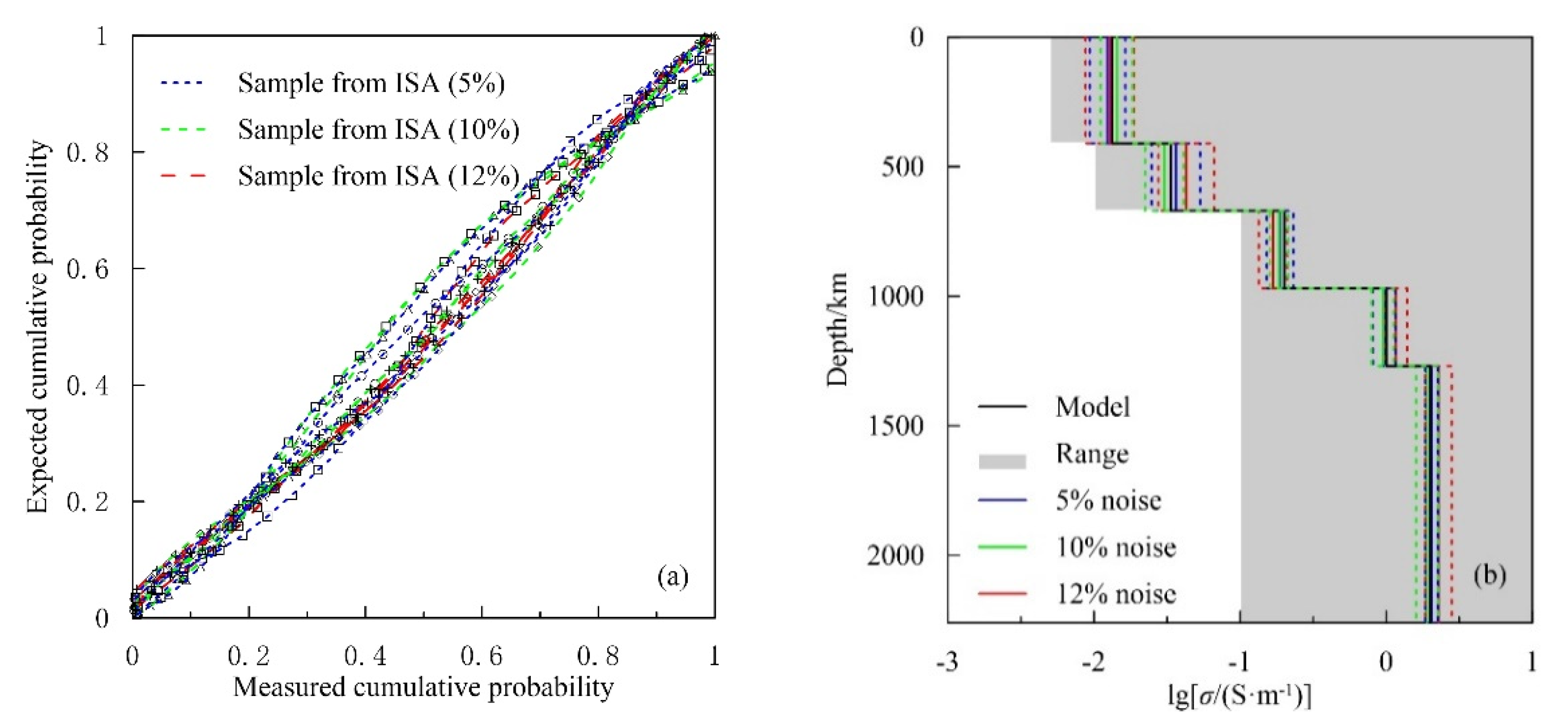
During the ISA inversion, the final inversion model is controlled by the choice of RMSmax which is dependent on the noise level of observed data. Because our data contain noises, the reliability of our inversion model should be evaluated. In order to do so, we use synthetic data to illustrate the issue: 5%, 10%, and 12% different Gaussian noises are added to the theoretical C-response in Figure 8. These noises levels cover all possible noises in the studying data. All inversion parameters except for RMSmax are the same as those in Section 3. Noise increasing demands a larger RMSmax; for the three different noise levels, after numerical tests, according to [26], the following are set: RMS5%max = 0.08, RMS10%max = 0.125, RMS12%max = 0.135. Figure 11 shows the data fitting of different noises. The fitting difference obtained by the final inversion is 0.075, 0.119, 0.121 in response to the increase in the noise level. However, it can be seen from Figure 10 that the C-responses obtained by ISA inversion within the acceptable noise levels for the theoretical data are fitted very well.
The inversion models are illustrated in Figure 12. Figure 12a displays the P-P diagram obtained by inversion of the conductivity of the four layers under three noise conditions. By observing the P-P diagram, we know that the effective model parameters obtained by the inversion basically conform to the lognormal distribution. Moreover, under the current noise level, the inversion result is basically not affected by noise. Figure 12b shows the final conductivity model and the reliability interval. It can be seen that although it is affected by different noises, the true values are all within the reliable range. In addition, the results show that the inverted conductivity model basically coincides at 410 km below and 900 km below. On the one hand, these intervals may be in the weakly sensitive area of geomagnetic depth sounding, on the other hand, it may also reflect the ability of the method in this paper to suppress the influence of noise. In the vicinity of the depth of the transition zone, comparing the theoretical models, the inversion results better reflect the theoretical model parameters. It is worth pointing out that the noise level affects the inversion results. There is a tendency that the greater the noise, the worse the conductivity of the inversion and the larger the range of the reliability interval. Hence, when there is less than 12% noise in the data, the true model can be obtained by using the inversion method proposed by this paper. When the data noise increases again, the inverted conductivity profile will deviate greatly from the true profile, and the true profile may not be within the reliable interval. At this point, the inversion model in Figure 7 is reliable even when data contain acceptable noises.

4.3. Evidence of the Mantle Plume Beneath Tarim

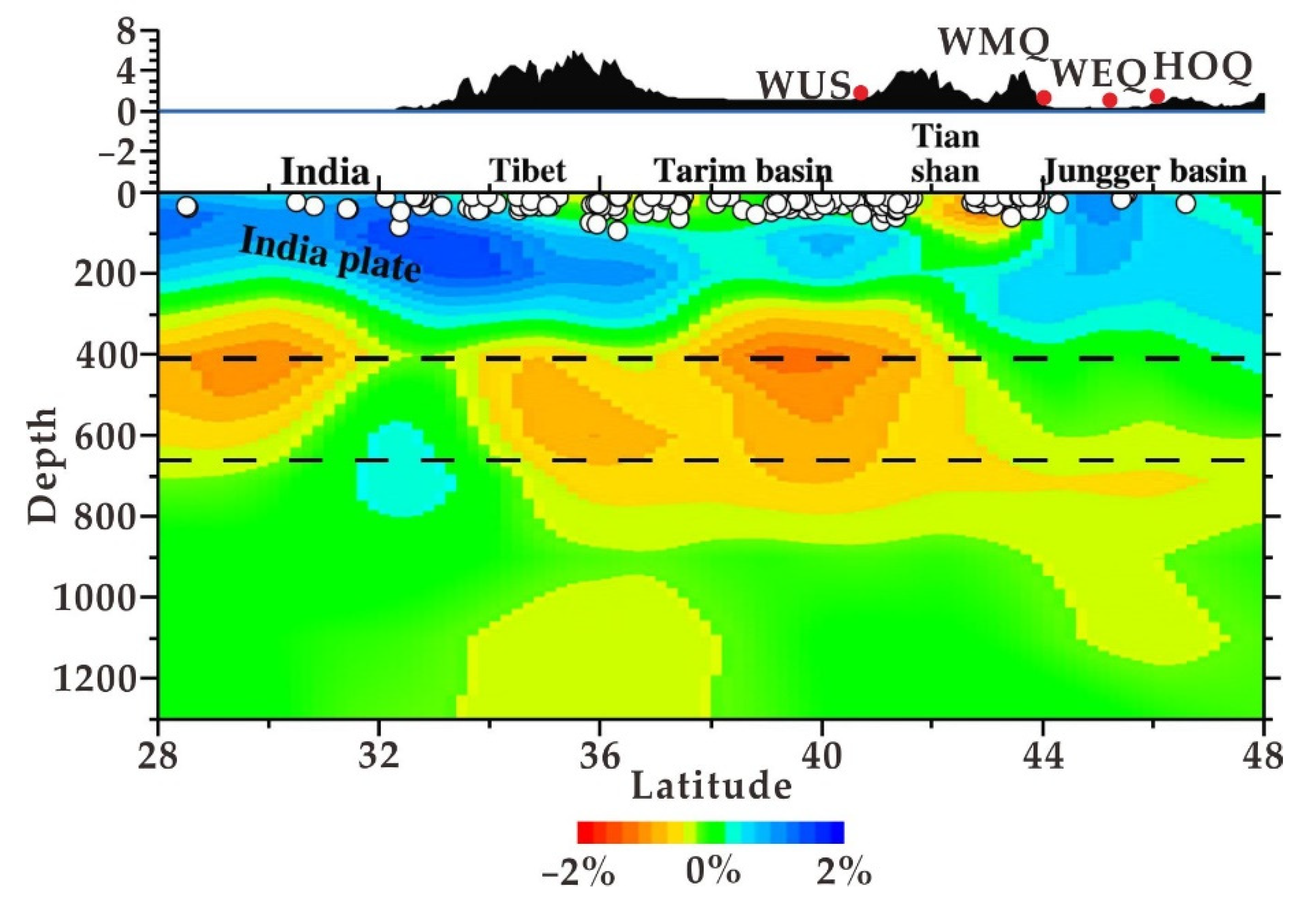
At present, a few people have noticed the low velocity anomaly beneath the Tarim Basin. Kosarev pointed out that this may indicate the existence of a mantle plume. One-dimensional conductivity inversion results show that there are obvious high conductivity anomalies in the upper mantle transition zone and the upper lower mantle in Tarim area. Compared with the results of previous seismic profiles (Figure 13), the author believes that the high conductivity anomaly beneath the Tarim Basin is reliable, and the high conductivity and low wave velocity indicate the existence of a temperature anomaly.
The increase in electrical conductivity in the mantle is usually explained by an increase in the water content and/or an increase in temperature. The minerals in the mantle transition zone have a high water content, which can reach 2.0 wt% [45]. Since the significant increase in the water content in the transition zone is usually related to the dehydration of the detained plate, and there is no clear plate detention in the Tarim transition zone, it is necessary to explain the high conductivity anomaly in the mantle transition zone through the increase in temperature. In order to discuss the temperature characteristics of the transition zone in the Tarim Basin, this paper uses Yoshino et al.’s high temperature and high pressure conductivity model
σ = σ OH exp ( H H R T t r ) + σ OP exp C w ( H p 0 α C w 1 / 3 R T t r ) ,
for the petrophysical calculation of the transition zone [43]. The conductivity profiles of 150 K, 300 K, and 650 K above the global average temperature of the mantle transition zone are obtained; σ is the volume conductivity, Cw is the water content, α is the geometric factor, R is the Boltzmann constant, R = 1.38 × 10⁻²³ J/K, Ttr is the thermodynamic temperature; σOH, σOP are the pre exponential factors, H is the activation enthalpy; the subscripts H and P are the electron jump conduction and proton conduction, respectively. The specific model parameters are shown in Table 2.
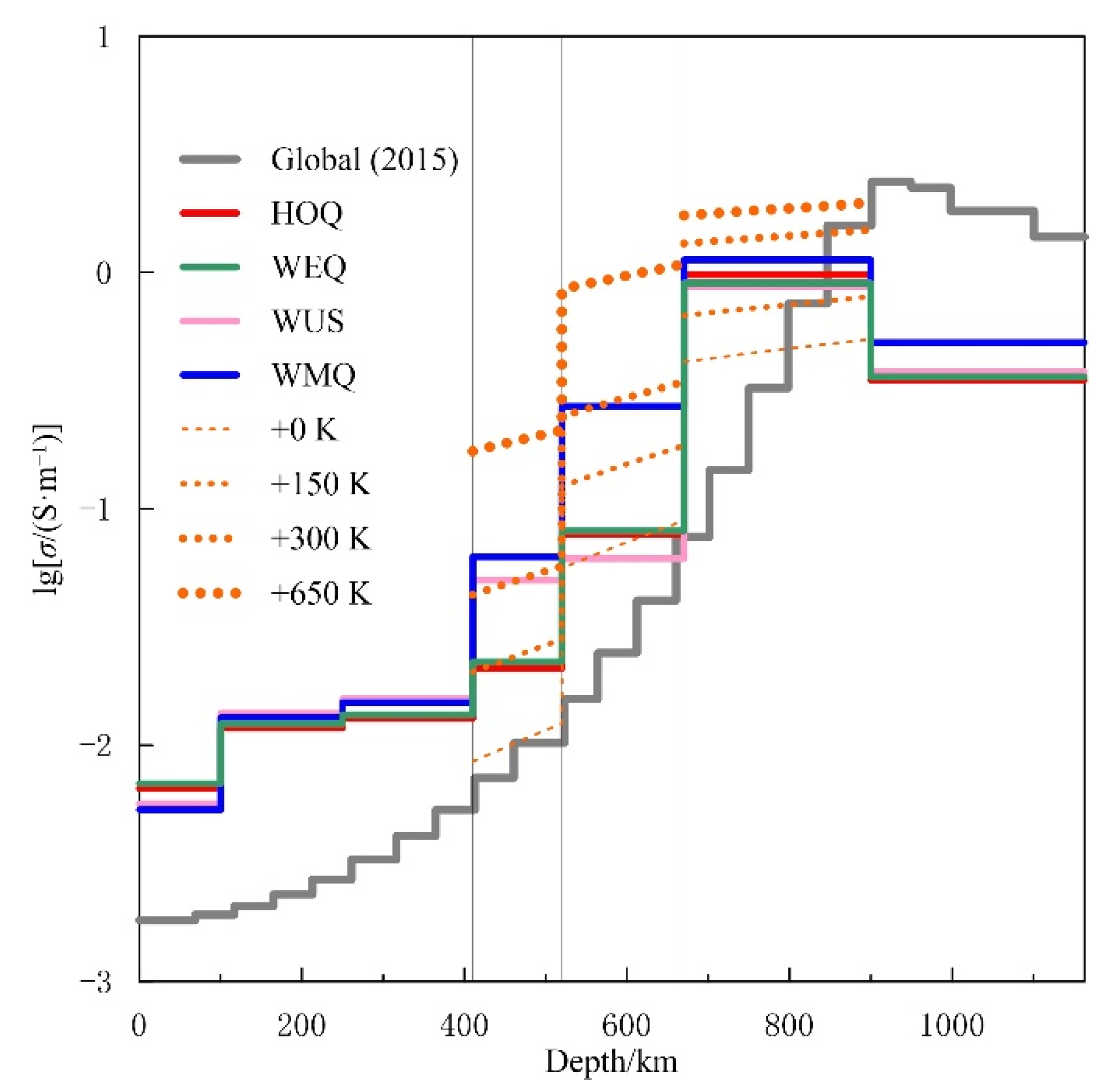
The water content in the lower mantle is extremely low, not exceeding 20 ppm [46], and there are currently very few experiments on the conductivity mechanism of the water-bearing rocks there. Therefore, when explaining the causes of high conductivity anomalies in the lower mantle beneath the Tarim area, only the temperature factor is considered. In this paper, we use Formula (13) from Sinmyo et al. [47] for petrophysical calculations for the upper layer of the lower mantle:
σ = σ 0 exp ( E a + P Δ V R T ) ,
where σ is the lower conductivity, σ0 is the pre-referential factor, σ0 = 74 S/m; Ea and ΔV are the activation energy and activation volume, respectively, where Ea = 0.7 eV, ΔV = −0.55 ± 0.01 cm3/mol. The values of temperature T and pressure P at different depths in the lower mantle can be found in [48]. According to Formula (12), the conductivity of the lower mantle is calculated at normal temperature, +150 K, +300 K, and +650 K, as shown in Figure 14. At the 660 km interface at the top of the lower mantle, the global average temperature is about 1925 K [43], and the electrical conductivity under the four stations around the Tarim area corresponds to the electrical conductivity after the temperature rises by 150–450 K. This shows that the temperature at the top of the lower mantle in the Tarim area has increased by at least 150 K.
It is shown in Figure 1 that the geomagnetic stations we use are distributed near the seismic profile. Figure 13 is the vertical section of the primary wave velocity disturbance corresponding to the profile. The seismic profile is from Huang’s article. It can be seen that there is an obvious low velocity anomaly at 410 km below the Tarim Basin; there is a high conductivity anomaly at 410–520 km in the one-dimensional conductivity profile of WUS station, which almost coincides with the seismic profile; and there is a good corresponding relationship between the two. We speculate that the temperature of WUS station is higher than the global average of 300 K. The WEQ/HOQ station is far from the high temperature anomaly body accumulated at the interface of 410 km, which makes the temperature increase by only 150 K. The location of the 660 km interface penetrated by the rising hot matter may be close to the WMQ station, which is the reason why the conductivity and temperature of WMQ are higher than those at the other three stations in the range of 520–660 km. The four stations have high conductivity anomalies at the top of the lower mantle. Combined with the banded low velocity anomaly at the top of the lower mantle in Figure 13, it is speculated that due to the influence of the greater resistance of the 660 km interface, the thermal material will accumulate at the top of the lower mantle and will have a larger area, and even the thermal material will appear below the HOQ and WEQ stations.
According to the high conductivity of the upper part of the lower mantle obtained by our one-dimensional geomagnetic depth inversion, combined with the low velocity anomaly obtained by previous seismic methods, it is inferred that there is a high temperature upwelling beneath the Tarim Basin, which is hindered by the 660 km interface and accumulates at the top of the lower mantle, and upwelling occurs through the interface near WMQ and then accumulates at the 410 km interface. Moreover, the accumulation of hot material at 410 km can also be seen under Hainan volcano [3]. Therefore, the inversion results can be used as electrical evidence to speculate that there may be mantle plumes beneath the Tarim Basin.

5. Conclusions

In this paper, a simulated annealing algorithm combined with statistical analysis technology is used to carry out one-dimensional inversion of four stations in Tarim area. The inversion test results of theoretical data show that the simulated annealing inversion method combined with statistical analysis has stable inversion results, a strong ability to reduce noise, and the ability to restore the conductivity profile of the Tarim Basin. Based on the inversion of the measured data of four stations around Tarim, the conductivity model under the station is obtained. The results show that the overall conductivity in Tarim area is higher than the global average, especially at the top of the lower mantle and the top of the mantle transition zone. Combined with the seismic results, we believe that it is in a high temperature state in the depth range of high conductivity below Tarim. It is speculated that there may be a mantle plume beneath the Tarim Basin.

Author Contributions

Data curation, X.L.; writing—original draft preparation, J.G.; supervision, X.W. All authors have read and agreed to the published version of the manuscript.

Funding

This research received no external funding.

Institutional Review Board Statement

The target of our research is not humans and animals.

Informed Consent Statement

The target of our research is not humans and animals.

Data Availability Statement

Restrictions apply to the availability of these data. Data was obtained from China Geomagnetic Network Center and are available from the authors with the permission of China Geomagnetic Network Center.

Acknowledgments

The BIRRP software package was provided by Chave A D, and the geomagnetic data were provided by the national network center. At the same time, we thank the reviewers and editors for their valuable comments on this paper, which enriched and completed the presented research.

Conflicts of Interest

The authors declare no conflict of interest.

References

  1. Xu, Z.Q.; Li, S.T.; Zhang, J.X.; Yang, J.S.; He, B.Z.; Li, H.B. Paleo-Asian and Tethyan tectonic systems with docking the Tarim block. Acta Pet. Sin. 2011, 27, 1–22. [Google Scholar]
  2. Huang, J. High-resolution mantle tomography of China and surrounding regions. J. Geophys. Res. Solid Earth 2006, 111, B09305. [Google Scholar] [CrossRef]
  3. Wei, W.; Zhao, D. Intraplate volcanism and mantle dynamics of Mainland China: New constraints from shear-wave to-mography. J. Asian Earth Sci. 2020, 188, 104103. [Google Scholar] [CrossRef]
  4. Kosarev, G.; Oreshin, S.; Vinnik, L.; Makeyeva, L. Mantle transition zone beneath the central Tien Shan: Lithospheric delamination and mantle plumes. Tectonophysics 2018, 723, 172–177. [Google Scholar] [CrossRef]
  5. Morgan, W.J. Convection Plumes in the Lower Mantle. Nature 1971, 230, 42–43. [Google Scholar] [CrossRef]
  6. Morgan, W.J. Deep Mantle Convection Plumes and Plate Motions. Aapg Bull. 1972, 56, 203–213. [Google Scholar]
  7. Griffiths, R.W. Stirring and structure in mantle starting plumes. Earth Planet. Sci. Lett. 1990, 99, 66–78. [Google Scholar] [CrossRef]
  8. Griffiths, R.W.; Campbell, I.H. Interaction of mantle plume heads with the Earth’s surface and onset of small-scale convection. J. Geophys. Res. 1991, 96, 18295–18310. [Google Scholar] [CrossRef]
  9. Campbell, I.H. Identification of ancient mantle plumes. Spec. Pap. Geol. Soc. Am. 2001, 352, 5–21. [Google Scholar]
  10. Pirajno, F.; Ernst, R.E.; Borisenko, A.S.; Fedoseev, G.; Naumov, E.A. Intraplate magmatism in Central Asia and China and associated metallogeny. Ore Geol. Rev. 2009, 35, 114–136. [Google Scholar] [CrossRef]
  11. Püthe, C.; Kuvshinov, A.; Khan, A.; Olsen, N. A new model of Earth’s radial conductivity structure derived from over 10 yr of satellite and observatory magnetic data. Geophys. J. Int. 2015, 203, 1864–1872. [Google Scholar] [CrossRef] [Green Version]
  12. Olsen, N. The electrical conductivity of the mantle beneath Europe derived from C-responses from 3 to 720 hr. Geophys. J. Int. 1998, 133, 298–308. [Google Scholar] [CrossRef] [Green Version]
  13. Kuvshinov, A.; Olsen, N. A global model of mantle conductivity derived from 5 years of CHAMP, Orsted, and SAC-C magnetic data. Geophys. Res. Lett. 2006, 33, L18301. [Google Scholar] [CrossRef]
  14. Ribaudo, J.T. Flexible Finite-Element Modeling of Global Geomagnetic Depth Sounding. Ph.D. Thesis, University of California, San Diego, CA, USA, 2011. [Google Scholar]
  15. Armadillo, E.; Bozzo, E.; Cerv, V.; De Santis, A.; Di Mauro, D.; Gambetta, M.; Meloni, A.; Pek, J.; Speranza, F. Geomagnetic depth sounding in the Northern Apennines (Italy). Earth Planets Space 2001, 53, 385–396. [Google Scholar] [CrossRef] [Green Version]
  16. Sun, J.; Egbert, G.D. A thin-sheet model for global electromagnetic induction. Geophys. J. Int. 2012, 189, 343–356. [Google Scholar] [CrossRef]
  17. Xu, G.J.; Tang, J.; Huang, Q.H. Study on the conductivity structure of the upper mantle and transition zone beneath North China. Chin. J. Geophys. (Chin.) 2015, 58, 566–575. [Google Scholar]
  18. Munch, F.D.; Grayver, A.; Kuvshinov, A.; Khan, A. Stochastic Inversion of Geomagnetic Observatory Data Including Rigorous Treatment of the Ocean Induction Effect with Implications for Transition Zone Water Content and Thermal Structure. J. Geophys. Res. 2017, 123, 31–51. [Google Scholar] [CrossRef]
  19. Zhang, Y.H.; Weng, A.H.; LI, S.W.; Yang, Y.; Tang, Y.; Liu, Y. Electrical conductivity in the mantle transition zone beneath Eastern China derived from L1-Norm C-responses. Geophys. J. Int. 2019, 221, 1110–1124. [Google Scholar] [CrossRef]
  20. Kelbert, A.; Schultz, A.; Egbert, G. Global electromagnetic induction constraints on transition-zone water content variations. Nature 2009, 460, 1003–1006. [Google Scholar] [CrossRef]
  21. Kuvshinov, A.; Semenov, A. Global 3-D imaging of mantle electrical conductivity based on inversion of observatory C-responses—I. An approach and its verification. Geophys. J. Int. 2012, 189, 1335–1352. [Google Scholar] [CrossRef] [Green Version]
  22. Semenov, A.; Kuvshinov, A. Global 3-D imaging of mantle conductivity based on inversion of observatory C-responses—II. Data analysis and results. Geophys. J. Int. 2012, 191, 965–992. [Google Scholar]
  23. Rothman, D.H. Nonlinear inversion, statistical mechanics, and residual statics estimation. Geophysics 1985, 50, 2784–2796. [Google Scholar] [CrossRef]
  24. Rothman, D.H. Automatic estimation of large residual statics corrections. Geophysics 1986, 51, 332–346. [Google Scholar] [CrossRef]
  25. Sen, M.K.; Bhattacharya, B.B.; Stoffa, P.L. Nonlinear inversion of resistivity sounding data. Geophysics 1993, 58, 496–507. [Google Scholar] [CrossRef]
  26. Sharma, S.P.; Kaikkonen, P. Appraisal of equivalence and suppression problems in 1D EM and DC measurements using global optimization and joint inversion. Geophys. Prospect. 1999, 47, 219–249. [Google Scholar] [CrossRef]
  27. Sharma, S.P.; Kaikkonen, P. Two-dimensional non-linear inversion of VLF-R data using simulated annealing. Geophys. J. Int. 1998, 133, 649–668. [Google Scholar] [CrossRef] [Green Version]
  28. Vedanti, N.; Srivastava, R.P.; Sagode, J.; Dimri, V. An efficient 1D Occam’s inversion algorithm using analytically computed first- and second-order derivatives for DC resistivity soundings. Comput. Geosci. 2005, 31, 319–328. [Google Scholar] [CrossRef]
  29. Banks, R.J. Geomagnetic Variations and the Electrical Conductivity of the Upper Mantle. Geophys. J. Int. 1969, 17, 457–487. [Google Scholar] [CrossRef] [Green Version]
  30. Tarits, P. Electromagnetic studies of global geodynamic processes. Surv. Geophys. 1994, 15, 209–238. [Google Scholar] [CrossRef]
  31. Li, S.W.; Weng, A.H.; Zhang, Y.H. Evidence of Bermuda Hot and Wet Upwelling from Novel Three-Dimensional Global Mantle Electrical Conductivity Image. Geochem. Geophys. Geosystems 2020, 21, 6. [Google Scholar] [CrossRef]
  32. Zhang, Y.H. The Structure of the Pacific Stagnant Plate in the Mantle of Eastern China Revealed by Three-Dimensional Geomagnetic Depth Sounding Images and Its Significance. Ph.D. Thesis, Jilin University, Changchun, China, 2020. [Google Scholar]
  33. Chave, A.D.; Thomson, D.J. Bounded Influence Magnetotelluric Response Function Estimation. Geophys. J. Int. 2004, 157, 988–1006. [Google Scholar] [CrossRef]
  34. Ingber, L. Very fast simulated re-annealing. Math. Comput. Model. 1989, 12, 967–973. [Google Scholar] [CrossRef] [Green Version]
  35. Srivastava, S.P. Theory of the Magnetotelluric Method for a Spherical Conductor. Geophys. J. Int. 1966, 11, 373–387. [Google Scholar] [CrossRef] [Green Version]
  36. Yoshino, T.; Katsura, T. Electrical Conductivity of Mantle Minerals: Role of Water in Conductivity Anomalies. Annu. Rev. Earth Planet. Sci. 2013, 41, 605. [Google Scholar] [CrossRef]
  37. Gelfand, S.B.; Mitter, S.K. Simulated annealing type algorithms for multivariate optimization. Algorithmica 1991, 6, 419–436. [Google Scholar] [CrossRef] [Green Version]
  38. Sharma, S.P. VFSARES-a very fast simulated annealing FORTRAN program for interpretation of 1-D DC resistivity sounding data from various electrode arrays. Comput. Geosci. 2012, 42, 177–188. [Google Scholar] [CrossRef]
  39. Ma, F.; Liu, L.; Yan, H. Application of the Statistical Analysis in Researching the Type of Motherrock in the West Strata of Songliao Basin. Glob. Geol. 2003, 22, 331–338. [Google Scholar]
  40. Li, J.P.; Weng, A.H.; Li, S.W.; Yang, Y.; Tang, Y.; Zhang, Y.H.; College of Geo Exploration Sciencesand Technology. The Influence of Ocean Effect on Geomagnetic Observations in Coastal Areas of China:A Case Study of the Guangzhou Observatory. Chin. J. Geophys. (Chin.) 2018, 61, 649–658. [Google Scholar]
  41. Kuvshinov, A.V.; Olsen, N.; Avdeev, D.B.; Olsen, N. Electromagnetic induction in the oceans and the anomalous behaviour of coastal C-responses for periods up to 20 days. Geophys. Res. Lett. 2002, 29, 1–4. [Google Scholar] [CrossRef]
  42. Shimizu, H.; Koyama, T.; Baba, K.; Utada, H. Revised 1-D mantle electrical conductivity structure beneath the north Pacific. Geophys. J. Int. 2010, 180, 1030–1048. [Google Scholar] [CrossRef]
  43. Yoshino, T.; Manthilake, G.; Matsuzaki, T.; Katsura, T. Dry Mantle Transition Zone Inferred from the Conductivity of Wadsleyite and Ringwoodite. Nature 2008, 451, 326–329. [Google Scholar] [CrossRef] [PubMed]
  44. Püthe, C.; Kuvshinov, A. Mapping 3-D mantle electrical conductivity from space: A new 3-D inversion scheme based on analysis of matrix Q-responses. Geophys. J. Int. 2014, 197, 768–784. [Google Scholar] [CrossRef] [Green Version]
  45. Williams, Q.; Hemley, R.J. Hydrogen in the deep Earth. Annu. Rev. Earth Planet. Sci. 2001, 29, 365–418. [Google Scholar] [CrossRef] [Green Version]
  46. Hirschmann, M.M.; Tenner, T.; Aubaud, C.; Withers, A.C. Dehydration melting of nominally anhydrous mantle: The primacy of partitioning. Phys. Earth Planet. Inter. 2009, 176, 54–68. [Google Scholar] [CrossRef]
  47. Sinmyo, R.; Pesce, G.; Greenberg, E.; McCammon, C.; Dubrovinsky, L. Lower Mantle Electrical Conductivity Based on Measurements of Al, Fe-Bearing Perovskite under Lower Mantle Conditions. Earth Planet. Sci. Lett. 2014, 393, 165–172. [Google Scholar] [CrossRef]
  48. Xu, Y.; Shankland, T.J.; Poe, B.T. Laboratory-based electrical conductivity in the Earth’s mantle. J. Geophys. Res. Solid Earth 2000, 105, 27865–27875. [Google Scholar] [CrossRef]
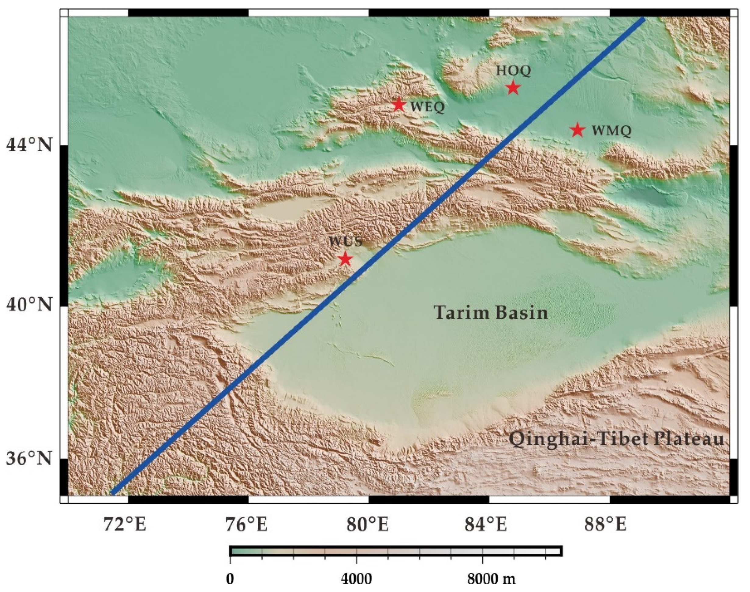
Figure 1. Location of geomagnetic observation stations. The red star represents the station; the blue solid line is the position of the vertical section of the primary wave velocity disturbance obtained by Huang [2].
Applsci 11 00893 g001
Figure 2. Three-component geomagnetic field recording signals from the WUS, WMQ, WEQ, and HOQ stations.
Applsci 11 00893 g002
Figure 3. C-responses at HOQ, WMQ, WEQ, and WUS stations estimated by the BIRRP software package [33]. The top panel shows the square consistency; middle and bottom panels are real and imaginary parts of the C-responses.
Applsci 11 00893 g003
Figure 4. The influence of the model constraint ranges on the SA inversion results. The shaded area denotes the parameter constraint range, the dashed line represents the theoretical real value (black or red), and the solid lines represent the convergence of two inversion variables in the SA inversion.
Applsci 11 00893 g004
Figure 5. The log-normal distribution histogram of the σ4 samples in the SA inversion. The inset is the P-P graph of the lognormal probability distribution of the σ4 samples. The abscissa of the subgraph is the measured cumulative probability density, and the ordinate is the expected cumulative probability density.
Applsci 11 00893 g005
Figure 6. The ISA inversion fitting of the C-response over WMQ (a), WUS (b), WEQ (c), and HOQ (d) stations.
Applsci 11 00893 g006
Figure 7. Conductivity depth profiles beneath HOQ, WEQ, WUS, and WMQ stations obtained by ISA inversion. The shaded zone is the parameter variation range; the dashed line indicates the reliability intervals estimated after inversion.
Applsci 11 00893 g007
Figure 8. The C response of the theoretical model in the inset. The shaded part in the sub-picture is the change interval of the conductivity parameter.
Applsci 11 00893 g008
Figure 9. The parameters of the theoretical model change in the SA inversion. (a) RMS; (b) σ1; (c) σ2; (d) σ3; (e) σ4; (f) σ5.
Applsci 11 00893 g009
Figure 10. Stability assessments of the ISA inversion method. (a) The fit of the C-response obtained by SA and ISA inversion; (b) The conductivity model obtained by SA and ISA inversion; the blue dashed line (three bars) represents the SA inversion result; the red solid line represents the ISA inversion results (three lines basically coincide), the red dotted line represents the reliable interval of the ISA results.
Applsci 11 00893 g010
Figure 11. The C-response inversion and fitting under different noise levels. (a) Noise is 5%; (b) Noise is 10%; (c) Noise is 12%.
Applsci 11 00893 g011
Figure 12. Inversion results of data containing different levels of noise. (a) The P-P diagram of the inversion results of the conductivity of the five layers at three noise levels, in which the circle, square, triangle, and cross correspond to σ1, σ2, σ3, σ4, σ5 in turn; (b) The final inversion model; the dashed lines corresponding to different colors are the reliability intervals.
Applsci 11 00893 g012
Figure 13. Vertical cross-sections of P wave velocity perturbations along the profiles shown in Figure 1 [2]. The surface along the profile is shown at the top of the cross section. White dots show the earthquakes that occurred within a 50-km radius from each profile. The velocity perturbation scale is shown at the bottom. The dashed black lines denote the 410 km and 660 km discontinuities. The red dots are a projection along latitude.
Applsci 11 00893 g013
Figure 14. Conductivity at 660–900 km. The global average conductivity profile is from [11]. Four orange dashed lines represent the conductivity corresponding to increasing temperatures.
Applsci 11 00893 g014
Table 1. Information of the four geomagnetic stations in Northwest China.
CodeStationGG-Lat (°)GG-Long (°)GM-Lat (°)GM-Long (°)Length
WuShiWUS41.20179.21632.168154.712007–2016
WenQuanWEQ44.96181.00435.780156.732007–2016
HongQianHOQ45.35984.79135.930160.062007–2016
UrumqiWMQ44.36086.94034.811161.822007–2018
GG, geodetic geographic coordinate system; GM, coordinate system.
Table 2. The parameter values used in the petrophysical model in Formula (18).
MineralσOH(S/m)HH(eV)σOP(S/m)Hp0(eV)α
Wadsleyite399(311)149(10)7.74(4.08)0.68(3)0.02(2)
Ringwoodite838(442)1.36(5)27.7(9.6)1.12(3)0.67(3)
Publisher’s Note: MDPI stays neutral with regard to jurisdictional claims in published maps and institutional affiliations.