Article

Analysis of Polygonal Vortex Flows in a Cylinder with a Rotating Bottom

1
Physics Department, NRCN, P.O.B. 9001, Beer-Sheva 84190, Israel
2
Department of Mechanical Engineering, Ben-Gurion University of the Negev, Beer-Sheva 84105, Israel
3
Technology Division, NRCN, P.O.B. 9001, Beer-Sheva 84190, Israel
4
DEN-STMF, CEA, Université Paris-Saclay, F-91191 Gif-sur-Yvette, France
*
Author to whom correspondence should be addressed.
Appl. Sci. 2021, 11(3), 1348; https://doi.org/10.3390/app11031348
Submission received: 1 January 2021 / Revised: 23 January 2021 / Accepted: 27 January 2021 / Published: 2 February 2021
(This article belongs to the Section Mechanical Engineering)

Abstract

:
The present paper provides a physically sound numerical modeling of liquid flows experimentally observed inside a vertical circular cylinder with a stationary envelope, rotating bottom and open top. In these flows, the resulting vortex depth may be such that the rotating bottom disk becomes partially exposed, and rather peculiar polygon shapes appear. The parameters and features of this work are chosen based on a careful analysis of the literature. Accordingly, the cylinder inner radius is 145 mm and the initial water height is 60 mm. The experiments with bottom disk rotation frequencies of 3.0, 3.4, 4.0 and 4.6 Hz are simulated. The chosen frequency range encompasses the regions of ellipse and triangle shapes as observed in the experimental studies reported in the literature. The free surface flow is expected to be turbulent, with the Reynolds number of O(105). The Large Eddy Simulation (LES) is adopted as the numerical approach, with a localized dynamic Subgrid-Scale Stresses (SGS) model including an energy equation. Since the flow obviously requires a surface tracking or capturing method, a volume-of-fluid (VOF) approach has been chosen based on the findings, where this method provided stable shapes in the ranges of parameters found in the corresponding experiments. Expected ellipse and triangle shapes are revealed and analyzed. A detailed character of the numerical results allows for an in-depth discussion and analysis of the mechanisms and features which accompany the characteristic shapes and their alterations. As a result, a unique insight into the polygon flow structures is provided.

1. Introduction

Fluid flows that include vortices widely occur in nature and in many engineering applications. The basic theory of vortex flows is well established, e.g., [1,2], and numerous basic solutions with some simplifications are available in the literature. For vortex flows in free surface liquids, deformation due to a submerged fluid vortex results in very complex, clearly asymmetric and thus three-dimensional flow fields, which are changing in space and time. Therefore, even very common and familiar-to-all cases, like a bathtub vortex, are rather difficult for analysis, and their theoretical studies are rare, e.g., [3].
One of the interesting model cases, for the first time apparently reported in the available literature in [4], is a vertical circular cylinder with a stationary side wall, rotating bottom and open top, as shown schematically in Figure 1a. This case is characterized by peculiar shapes, created by the free surface, including partial exposure of the rotating bottom, as illustrated in the figure using an example from the present study. As was pointed out in [4], “The receding water exposed part of the surface of the disk to air, whereby the line of intersection between the surfaces of the solid disk and the liquid outlined Kelvin’s static shapes of the core” (see [5]). In the three decades that followed, this phenomenon has been studied very extensively by a number of research groups. These studies have resulted in a significant body of work, from impressive images produced via visualization to quantitative characteristics related to rotation frequencies, shape transitions, hydrodynamic stability etc. Yet, an apparent absence in the literature of any numerical results for the highly distorted free surface vortex flows over partially exposed surfaces obviously impedes their better understanding.
In the present study, an attempt is made, for the first time in the available literature, to model numerically the free surface vortex flows over a rotating exposed bottom. The reported modeling is done based on a scrupulous analysis of the existing literature, especially the experimental works published on the subject during the last three decades.

1.1. Experimental Studies

The major experimental studies from the literature are summarized in Table 1. First experiments with water inside a stationary cylinder with a rotating bottom were reported in [4]. Under certain conditions, it was observed that the free surface reached the rotating disk and partially exposed it, producing shapes of polygons with varying numbers of corners, N. These shapes were stable for up to N = 6, such that if perturbed or even fully destroyed, they would restore their initial configurations. In [4], the polygons were mapped by their number of corners, “wave numbers”, as a function of the disk velocities and initial water heights. A range of disk velocities was found for each wave number. The experimental work [6] dealt with the impact of liquid viscosity on the phenomenon of free surface polygon formation, as two additional liquids, with the viscosities of 56.7 and 640 times higher than that of water, were used. The lower and upper boundaries of disk velocity for each range were found to increase linearly with the initial water height. Between two adjacent stable states, a mixed, time-dependent state was observed. This state was a superposition of the corresponding wave numbers, and was not stable, because each shape, with different wave number, was rotating at a different speed.
Free surface polygon formation, similar to the one earlier reported in [4,6], was independently confirmed in [7]. The experiments were conducted with water and ethylene glycol which has a 15 times higher viscosity and similar density, as compared with water. A phase diagram, showing the wave numbers as function of the initial height and the disk frequency, was reported. Linear dependence between the initial height and the limit frequencies for each range reported in [6] was observed in [7]. Close to the upper limit of the frequency range for each polygon, a transition state, in which the corners of the polygon changed periodically from N to N + 1 (in particular between N = 2 and N = 3), was observed. For N > 2, the free surface exposed typically the rotating disk and thus created a “dry” polygon [7]. For N = 2 and in some sub-cases of N = 3, the rotating disk was completely covered with water, creating a “wet” polygon. However, in their phase diagram, dry and wet polygons were not distinguished. Surface tension effects by adding surfactant into the fluid, also reported in [7], did not change the phase diagram significantly. Spiraling vortices, observed in the corners of the polygons, were interpreted as Görtler vortices. It was argued that the secondary flow was highly dependent on the singular corners created by the proximity of the rotating disk and the cylinder fixed walls. This makes the details of the flow very complicated, as noted in [7]. In a similar but smaller experimental set-up, the switching between circular and elliptical cross sections, N = 0 and N = 2, was investigated in [8]. Measuring the free surface height above the center of the rotating disk, several free surface states depending on the Reynolds number (defined as Re = ωR2/ν, where ω is the disk angular velocity, R is the cylinder radius and ν is the kinematic viscosity) were identified [8]. The results from the above studies indicate that the creation of the polygons, their shapes, stability and rotating velocity depend on the geometry of the experiment and on the Reynolds number. In an additional communication, the use of the Froude number, defined as Fr = ωr/(gr)0.5, where r is the bottom disk radius, was suggested in [12], which looks quite reasonable because free surface flows are considered. With the same experimental device and flow parameters as of [8], the free surface cross section transition by visualizing the flow pattern using anisotropic flakes was studied in [13]. The vertical cross section along the centerline of the cylinder was recorded. The orientation of the flakes, which were arranged along the principal strain in the flow, was used to observe the flow patterns. The measurements of the free surface level at the cylinder axis and the radial velocity profile, and the computation of the turbulent intensity as function of Re, were reported in [14].
The same experimental set-up as in [4,6], but with several rotating disk diameters, was employed in [15]. Beside the main vortex, secondary vortices were observed in the corners of the rotating polygons, as was previously reported in [7]. It was suggested that when the velocity of the disk is increased, the main and the secondary spiraling vortices intensify and cause the liquid to recede, thus forming a dry polygon. In other words, a polygon with N corners is equivalent to N secondary point vortices rotating around the main polygon, forming the vortex. In the experiments of [4,6,7,15], the highest wave number polygon observed was with N = 6. It was argued that the reason for not showing polygons with the wave numbers higher than 6 is that the secondary vortices are not stable according to [16,17]. The ratio of the polygon to disk angular velocities was found to decrease with an increase in the Froude number (with the initial height as the characteristic length) and to increase with N [15].
Different parameters affecting creation and transition of the polygons were studied in [18,19,20]. In particular, it was indicated that a smoother surface delays the creation of the polygons. Then, the radial distance from the center to the pattern was determined for each azimuthal angle as function of time, using image processing. The functions were transformed to the frequency domain for each angle and averaged. It was found that before the transition, the dominant frequency corresponded to the rotation of the N polygon. Other frequencies were few orders of magnitude lower than the N frequency. Increasing the rotating disk frequency caused the frequency of N + 1 to be more dominant than the frequency of N, whereas these two frequencies are coupled.
The study [21] focused their attention on the formation of dry and wet polygons with N = 3, i.e., a triangle. Their experimental device was similar to that of [7]. Similar to [4,15], it was observed that the formation of dry polygons did not depend on the initial conditions: the same shape was obtained when starting from the rest or from a circular shape, or when destroying the stable polygon without changing the disk rotation speed. To investigate the evolution of the dry triangle polygon, the Fourier coefficients of the contour radial coordinate were computed with time, and it was shown that the polygon formation is caused by linear instability. In the circular state prior to the formation of the triangle, the azimuthal and radial velocities on the free surface were measured. It was shown that the azimuthal velocity has a profile of Rankine vortex, as predicted analytically assuming the flow is inviscid. In the triangle state the angular velocity was much higher than the one that results from three-point vortices at the corners of the triangle in the triangle rotating reference frame. Thus, it was argued that the point secondary vortices used in the Havelock’s model [17] without a central vortex cannot describe the flow. In an additional communication, it was shown that the maximum vorticity was obtained in the center of the spiraling (secondary) vortices, and a plateau of the vorticity exists between them [21]. Using the experimental set-up of [15], it was argued in [22] that the velocity of the N spiraling vortices causes the circular shape of the primary vortex to deform to the polygon shapes. Using PIV, the rotation rate of the polygon was measured and compared with Havelock’s model of point vortices [17]. It was found that taking into account the angular velocity of the flow from the solid body rotation region, in addition to the angular velocity proposed in [17], yields good agreement with the angular velocity at the center of the spiraling vortices extracted from PIV measurements.
The formation of polygons in a cylinder in which the bottom plate and the vertical walls could be rotated independently was investigated experimentally in [10]. The results for stationary walls were compared with those of [4,6,7]. “Excitability” of the polygons was explored. Similar to the works [4,6,7], multi-stability was observed in the experiments: for most of the parameters, a stable state, which did not depend on the initial conditions, was found; however, in some of the transitions, two or more stable states were observed, for the same frequency. The suggested explanation for this effect was the dependence on initial conditions at these certain frequencies. The excitability was evident by a number of unstable states when perturbing the flow.
An experimental set-up with a cylinder radius in between the radii used by [7] was employed in [23]. They also observed a linear dependence between the initial water height and the transition disk rotation frequency. Like in [4,15], it was found that the transition between an ellipse and a triangle was unstable, with changes between a distorted ellipse and an elongated triangle, which also rotated at different rates.
The issue of the viscosity effect regained attention in [11]. The reason is that the main assumption in most analytical works (surveyed below) is that the fluid is inviscid. It was argued that in addition to Froude number, the Taylor number (which is the ratio of the centrifugal force to the viscosity force) is governing the flow. It was found that increasing the viscosity of the fluid during rotation results in decreasing the range of disk velocities for patterns with higher N. The viscosity had no effect on the ratio between the frequencies of the polygons and the disk. In [24], it was shown experimentally that increasing the viscosity of the fluid does not influence the transition mechanism presented by [18,20], thus arguing that the behavior of the flow can be described as rotating point vortices, as shown in [15].
The above surveyed experimental studies on free surface flows in cylinders with rotating bottom disk show mostly qualitative rather than quantitative agreement in the observed phenomena: same polygon shapes in the stable states, linear dependence between the initial water height and the disk frequencies for the transition between the neighboring polygon shapes, and independence of the stable states of the initial conditions for the most of experimental conditions. In some studies, the transition between the shapes was gradual (as in [6,15]) and in others it occurred in an oscillatory manner (as in [7]) or periodically (as in [25]). In any case, the transition was characterized by combined N and N + 1 shapes.

1.2. Analytical Modeling

Along with the experimental works, analytical models were developed in an attempt to understand the phenomena involved in polygon shapes’ formation and transition. Two-dimensional rotating flow was considered in [26] in two cases: a hollow potential vortex (which simulates a dry polygon) and a Rankine vortex (which simulates a wet polygon). By applying a linear stability analysis, they obtained the phase velocity (defined as the ratio of the angular velocity, ω, to the wave number, N) and the polygon shape for each case. The predicted phase velocities in stable states for N = 3 and N = 4 showed reasonable agreement with the measurements reported in [6].
A hollow potential vortex but with three-dimensional perturbations was also considered in [27]. They solved numerically the corresponding Laplace equation along with the boundary conditions in a three-dimensional domain, and also suggested a simplified solution based on separate two-dimensional problems concerning rotation at the plane of the bottom disk and at the cylindrical surface, respectively. The linear stability analysis was applied to these two problems, yielding two types of waves: centrifugal waves for the first problem and gravity waves for the second one. It is shown that the instability occurs when the frequencies of the two kinds of waves are equal and the centrifugal wave travels backward relative to the mean wave. The predicted transition frequencies, obtained using both two- and three-dimensional models, reasonably agreed with the experimental results of [7]. In addition, the gravity waves were similar to the waves observed in [23]. The experimental findings of [28] support the predictions of [27] for transition between a circle and an ellipse shapes, with small discrepancies attributed to the region of solid body rotation that were not taken in account in the model. The model of [27] neglects the singular point between the rotating bottom and the fixed cylinder walls, implying that the instability is not affected by the flow details in the vicinity of the singular point. To support this idea, an experiment with liquid nitrogen rotating inside a hot kitchen pot was conducted [27]. The hot pot boiled the nitrogen layer in its immediate vicinity and thus practically eliminated the friction between the liquid and the boundaries, hence precluding singularity. Polygons were still observed, thus supporting the model assumption.
The model presented in [27] was extended in [29] and considered the Rankine vortex, rather than the potential vortex. It was suggested in [30] that rotating waves are cnoidal waves which result from the nonlinear equation of Korteweg–de Vries. The free surface polygon shapes instability was also a subject of analytical study in [31]. The global stability problem of [27] was extended further in [32]—more complex wave structures were found.

1.3. Numerical Modeling

Analytical modeling for the problem in question is obviously limited. Thus, numerical simulation should be very appealing. Remarkably, the literature that might be considered relevant in this sense is rather limited.
There exist numerical works on the configuration in question but they were focused on another phenomenon. It was experimentally observed, for Re < 4000 and h/R ≤ 4, where h is the initial water height, that the vortex, created by a rotating bottom disk, can be broken into recirculating bubbles [33]. This vortex breakdown is laminar and occurs under steady flow conditions. A possible bifurcation of streamline structures as function of Re and h/R, assuming axisymmetric flow and flat top surface was numerically derived in [34]. In [35], the flow was investigated numerically by direct solution of the Navier–Stokes equations without any symmetry assumption but again with flat free surface. It was shown that at Re = 6000, the flow is divided into two regions: in the inner region, the flow behaves as solid body rotation, while the flow in the outer region behaves as a jet along the cylinder wall and turns into the radial direction towards the inner region, causing unstable azimuthal modes. The same problem but allowing the free surface to deform slightly, corresponding to Fr = 0.1 and relative surface deformation of 0.012, was modeled in [36].
Modeling the problem with a flat free surface imposes a reflection symmetry on the flow, where the free surface serves as the reflection plane, as studied in [37,38]. Thus, a cylinder with double height (relative to the experimental cylinder) and with two co-rotating end-walls (Fr = 0) was modeled. Two aspect ratios were considered: a deep system with h/R = 2 and a shallow system with h/R = 0.25. It is shown that in the shallow system, solid body rotation exists in the inner region and meridional flow occurs in the outer region, whereas the deep system has meridional flow throughout the cylinder. The area near the axis consists of recirculation bubbles, as observed in [33]. The behavior was assumed to be of Hopf bifurcation type, studied earlier in, e.g., [34,39,40] for similar cases, and in [41] for stationary and rotating disks. The mechanism for the symmetry breaking in the deep system is due to azimuthal instability of the shear layer that is turning to the interior from the stationary cylinder, as was argued in [42]. The symmetry breaking has a reflection symmetry, therefore the flat free surface modeling, which imposes that reflection symmetry, can predict symmetry breaking of the experiments. For the shallow system, the instability mechanism is due to azimuthal instability in the interface between the solid body rotation zone and the meridional flow zone. In this case, the symmetry breaking has no reflection plane and cannot be predicted by the flat free surface model. It is worth noting that as shown experimentally, increasing the surface tension could stabilize the flow into axisymmetric state [37].
Obviously, numerical modeling at low Reynolds numbers cannot describe the experimentally observed free surface symmetry breaking and polygon shape formation where the typical Reynolds numbers are of the order of 105, as described in detail above. However, to the best of our knowledge, only very few studies have started to go in that direction. Moreover, significant simplifications continue to be used. Experiments with small h/R ratio (see Table 1) were conducted in [9]. A polygonal flow structure was reported to be created by spiraling vortices in the corners of the polygon. Experiments reported in [9] were modeled in [43] with direct numerical simulation (DNS) at Re up to 27,000 without free surface distortion. The model predicted well the first symmetry breaking from the experimental work of [9] for large h/r, but large discrepancies were obtained for small h/r. This was first attributed to the assumption of the flat free surface, but as was shown in [44] adding the deformation of the free surface did not improve the results. In [43], it was suspected that surface tension might be the cause for this disagreement. Following the definition given in [45] for the critical Reynolds number (ReNM = VL/ν) that governs the instability, they showed that, for every Reynolds number, ReNM remains constant by taking the characteristic velocity, V, as maximum velocity of the disk and the characteristic length, L, as the thickness of the shear layer, estimated as L = (Eh/4)1/4h, where Eh = ν/(ωh2) is the Ekman number.
The base flow, before the first symmetry breaking, was numerically simulated in [46] by direct solution of the Navier–Stokes equations, assuming a stream function. The equations were coupled to the free surface deformation and solved by an iterative process. The free surface deformation results agreed with those reported in [47] for Re = 900, but there was disagreement with the results of [36] for Re = 900 and 1500. In addition, the free surface deformation reported in [4,8], was qualitatively compared in [46] for the case before the symmetry breaking and without reaching the rotating disk. It was found that, due to the solid body rotation near the axis, the free surface deformed as a parabola and the free surface level decreased as the Reynolds number increased. To validate the results, experiments with Re of the order 1000 and Fr~1 were also conducted in [46]. It was shown that the experimentally found free surface deformation agreed with the numerical results.
Most recently, the base flow was studied numerically in [48], using the experimental conditions of [21]. First, the effects of the Fr and Re on the flow field were investigated [48]. It was found that for Froude number in the range of 0.01 to 1 (where the fluid almost touches the rotating disk in the latter case), the flow field far from the cylinder axis is not significantly influenced. Thus, beyond some exploratory computations dealing with perfectly symmetrical free surface vortices, the work in [48] concentrated on flow with flat free surface, thus reducing computational efforts. Accordingly, the attention focuses on meridional circulation, providing further confirmation of the computed boundary layers at Re = 1500 [49,50] and at higher Re (>10,000) [27].
The discussion presented above suggests that a detailed numerical analysis of rotating polygons should be used to shed new light on this challenging problem. Such simulation, which encompasses the appropriate ranges of the governing parameters, is reported in the present study. This work focuses on conditions where stable states were observed experimentally. The meaning of “stable” in this context is that for a given set of conditions, a certain shape is attained, and though it may vary, it always remains within the same polygon type (constant N).

2. Numerical Modeling

The experiments reported in [10] are chosen to be modeled in the present study. This means that the geometrical and flow parameters of their system were carefully reconstructed in this work. According to their results, the frequencies chosen for numerical modeling are within the ranges of stable ellipses and triangles observed experimentally. The simulations are done using the ANSYS Fluent -r19.0.0 software platform (2019) [51]. This software employing VOF technique to model free surface flows was found reliable in capturing the phenomena relevant to the present study—see, e.g., a recent publication [52].

2.1. Choice of the Numerical Approach

For the range of experimental conditions analyzed in the present study, the free surface of the rotating fluid was strongly deformed. Hence, the errors associated with employing non-deformable free shear boundary conditions might be expected to be significant. Moreover, as the free surface for the range of the experimental conditions modeled in the present study has assumed, among other cases, the shapes of ellipses and triangles (as in [10]), full asymmetric 3D calculations are performed. The flow in question is expected to be a turbulent free surface flow. As the Reynolds number based on the disk radius is of the order of 105, direct numerical simulation (DNS) is impractical. Employing Reynolds-averaged Navier-Stokes (RANS) equations, unsteady simulations have proven to be unrealistic as, in a preliminary study, they revealed no asymmetry in the shape of the free surface (these results are not shown for the sake of brevity). It was thus decided to use Large Eddy Simulation (LES). The essential specific details of the adopted approach are presented below.
Subgrid-Scale Stresses (SGS) model has to complement any LES calculation. A number of models for SGS calculation are available [53]. A localized dynamic model including an energy equation [54] was employed in the present study. The model solves a transport equation for the subgrid kinetic energy, while model coefficients are obtained using a localized dynamic procedure. The subgrid-scale kinetic energy, as implemented in Fluent, is defined as
k s g s = 1 2 u k 2 ¯ u ¯ k 2
which is obtained by contracting the subgrid-scale stress
τ i j ρ u i u j ¯ ρ u i ¯ u j ¯
The subgrid-scale eddy viscosity, μ t , is computed using k s g s as
μ t = C k ρ k s g s 1 / 2 Δ f S i j ¯
where Δ f is the filter size computed from the cell volume, Δ f V 1 / 3 . The subgrid-scale stress can be then written as follows:
τ i j 2 3 ρ k s g s δ i j = 2 C k ρ k s g s 1 / 2 Δ f S i j ¯
The subgrid-scale kinetic energy is obtained solving the following transport equation:
ρ k s g s ¯ t + ρ u j ¯ k s g s ¯ x j = τ i j u j ¯ x j C ε ρ k s g s 3 / 2 Δ f + x j μ t σ k k s g s x j
where C k and C ε are determined dynamically and σ k = 1 .
The localized dynamic model was found to be particularly important since it implies that in high-Reynolds-number flows, a relatively coarser grid (when compared with the algebraic LES model) can be used [54]. This model was successfully applied for modeling rotating shear flows [55].
Free surface fluid flows are usually computed employing interface capturing methods [56]. Two methods are widely employed: volume-of-fluid (VOF) approach [57] and level set method (LSM, [58]). The main strength of VOF methods is their ability to preserve mass [59], while the advantage of those based on level set is the accurate representation of the free surface normals and curvature [60].
The ability of combined LES and free surface capturing methods to predict free surface turbulent flows is demonstrated in a number of publications (e.g., [56]). The LSM was employed in [61] in conjunction with LES for turbulent open channel flow over fixed dunes. Two subgrid-scale models, namely, dynamic Smagorinsky and dynamic two-parameter one, were used. It was observed that the method was able to accurately and realistically calculate the unsteady free surface motion and also provided evidence of boils, upwelling and downdraft at the water surface. The results were relatively insensitive to the choice of the subgrid-scale model. Calculations on the flow past a cylinder protruding from the water surface at the Reynolds number Re = 2.7 × 10⁴ and the Froude numbers Fr = 0.2 and 0.8 were reported in [62]. A Lagrangian dynamic subgrid-scale model, complemented with LSM for capturing the free surface, was employed. The mean interface level and the root mean square (r.m.s.) of interface fluctuations from the simulation were reported to be in excellent agreement with the experimental results. Along with VOF and LSM methods, a number of hybrid techniques were developed for interface capturing. The coupled level set/volume-of-fluid (CLSVOF) method, as developed in [63], is applied when the free surface is expected to be highly complex. Results of a very recent work which deals with mechanisms of air-core vortex evolution in an intake flow are reported in [64].
Based on the literature analysis, the localized dynamic SGS model for LES turbulence model was used in the present study for simulating flows in an open static cylinder with a rotating bottom, partially filled with water. As for resolving the interface, this study started with employing the CLSVOF approach. However, an extensive investigation for the frequencies where stable ellipse and triangle polygons were experimentally observed in [10] revealed that the hybrid CLSVOF, while successfully capturing these shapes, could not ensure their stability. For this reason, the VOF method was used instead. This method was recently successfully applied in [65] to modeling of rotating free surface turbulent flow in a whirlpool including the phenomenon of phase separation. The tracking of the air–water interface is accomplished by the solution of an explicitly discretized continuity equation for the volume fraction. Geometric reconstruction scheme is used for the cells near the water–air interface. The scheme represents the interface between fluids using a piecewise-linear approach.
The VOF technique is employed to air and water immiscible fluids by solving a single set of momentum equations and tracking the volume fraction of each of the fluids throughout the domain. The tracking of the interface between the phases is accomplished by the solution of a continuity equation for the volume fraction of one of the two phases. For one of the phases, assuming incompressible fluids without mass transfer between the phases and without sources, this equation has the following form:
t α a + v ¯ a · α a = 0
As only air and water phases are present, the volume fractions of the two phases sum up to unity in each control volume:
α w + α a = 1
Implicit volume fraction formulation is chosen for time discretization in the present study. The following equation is solved for the secondary phase (water in this case) at each time step to obtain the face fluxes for all cells, including the interface:
α a n + 1 α a n Δ t V + f U f n + 1 α a , f n + 1 = 0
A single momentum equation is solved for the two phases with the properties, e.g., density, being calculated as void fraction weighted average of the two components. In the present work, VOF method is combined with a constant contact angle treatment (found appropriate in a number of applications—e.g., [66]) for the moving water boundaries on vertical walls and rotating bottom. Alternative treatment of the contact angle parameter can also be considered—e.g., recently published work [67] on application of dynamic contact angle formulation along with VOF method.
As will be demonstrated below, the chosen approach makes it possible to obtain stable shapes while all other simulated features correspond well with the experimental observations.

2.2. Computational Details

The experimental apparatus employed in [10] allowed simultaneous rotation of both the bottom disk and the cylindrical wall. In the present study, we focus on the cases where the cylindrical wall was kept static. The cylinder inner radius in the experiment was 145 mm. Experiments with only bottom plate rotation were performed with varying filling heights, from 30 to 80 mm. This study focuses on modeling the case with the initial water height of 60 mm. The experiments with bottom disk rotation frequencies of 3.0, 3.4, 4.0 and 4.6 Hz are simulated. The chosen frequency range encompasses the regions of ellipse and triangle shapes (two frequencies for each case) as observed in the experiment—see [10]. The explored values of governing dimensionless groups and other parameters are listed in Table 1, along with the corresponding data for the existing works.
The computational domain and grid employed in the present study are presented in Figure 1b. The base grid consisted of 1.1 million hexahedral cells built employing the O-grid technique. Appropriate mesh morphology generation is vital for an accurate solution, faster convergence and reduction in numerical diffusion. Hexahedra structured O-grid employed in the present study is characterized by regular connectivity and high space efficiency. The chosen grid is aligned in the main rotational direction of the flow in question, where possible, leading to more accurate results and a better convergence. The minimal orthogonal quality of the computational domain was 0.75 with the maximal grid aspect ratio being 12 in the limited region of the stationary cylinder boundary layer, where the prevailing flow direction is azimuthal, this aligned with the longer edge of the computational cells. Such a grid resolution, being fine in the radial direction, ensures correct representation of the flow in the boundary layer at the stationary cylinder walls. The grid was refined close to the rotating bottom disk and vertical stationary cylinder wall to capture better the flow details in the Ekman and Stewartson layers, respectively.
It is obvious that grid and time-step choice are of crucial importance for a reliable simulation of the expected complex flow fields. In this work, the following approach was adopted: the grid was refined using the LES index of quality (LESIQν), introduced in [68], as the criterion. The LESIQν is a dimensionless number between zero and unity, reflecting the ratio between resolved and total turbulent kinetic energy. According to [68,69], based on [70], an index of quality greater than 0.8 is considered a good LES, while 0.95 and higher may be considered a DNS. Figure 2a,b show the contours of instantaneous values of LESIQν for the fastest case of the present investigation, namely, of 4.6 Hz. Figure 2a shows the values of LESIQν for the free surface of the liquid, while Figure 2b shows its values in the vertical cross-section of the flow. One can see from the figures that LESIQν is above 0.8 practically everywhere, and in most locations, it is close to or above 0.9. A parameter, which may be used for ensuring temporal resolution of the simulation, is the Courant number. One can see from Figure 2c, for the same complex case of Figure 2b, that the Courant number is smaller than unity practically all over the simulated flow field. The only exceptions are the “corners”, i.e., the locations where the rotating disk meets with the stationary wall, but this effect does not influence the outcome of the simulations. Calculation using a grid refined further by the factor of 1.5 in all the three directions (3.3 times global refinement) was done with no appreciable difference in the results.
No-slip and no-penetration boundary conditions are applied on the rotating bottom disk and the vertical cylinder wall. The top boundary of the computational domain was defined as pressure outlet. As the domain height in all the computations was larger than the uppermost height reached by the water level, only air flow crossed the top boundary, without the liquid being “spilled” out from the computational domain. In fact, instantaneous velocity field shows some of the air leaving the computational domain, while the same amount is drawn back due to continuity constraint, since the flow is treated as incompressible.
For all the calculations performed for the current study, the initial water level was set to 60 mm by setting the volume fraction value to be unity below this height and zero in the volume above it. All the computations were initialized with both air and water being at rest with zero velocity field patched to the whole computational domain. A zero value of subgrid-scale kinetic energy field was set to the fluids at the beginning of each calculation. The cylinder bottom disc initial velocity was set to its desired value from the beginning of each calculation. The flow field was allowed to develop from the described initial conditions until a quasi-periodic state was reached. All the flow conditions discussed in the present study were observed after the initial developing stage was over.
The solution controls for the discretization of the governing equations were as follows. The Pressure-Implicit with Splitting of Operators (PISO) pressure–velocity coupling scheme was employed. This modification of Semi-Implicit Method for Pressure Linked Equations (SIMPLE) algorithm assures new velocities and fluxes satisfy momentum balance after the pressure correction is performed to fulfill the continuity constraint. Gradients of the scalar fields were computed using least squares cell-based algorithm. As VOF algorithm was employed for most part of the present study, and considering swirling flow field expected in the domain, the PREssure STaggering Option (PRESTO!) scheme was used for pressure interpolation. A second order central differencing scheme was chosen for momentum equation discretization. Subgrid kinetic energy was discretized using second order upwind scheme. Compressive volume fraction discretization was employed. Time formulation was bounded second-order implicit, employing 0.001 s time steps with 30 iterations per step. Under-relaxation factors for pressure, density, body-forces, momentum, volume fraction, subgrid kinetic energy and turbulent viscosity are chosen at their default values as 0.3, 1.0, 1.0, 0.7, 0.5, 0.8 and 1.0, respectively. Complete data files were saved every 0.1 s, while the animation of the free surface height contour maps and mesh view visualization were saved every 0.01 s. The chosen calculation scheme resulted in the continuity residuals drop at the end of every time step to the values of the order of 10−4 for the continuity equation, while the residuals were as low as about 10−8 for the rest of the conservation equations solved.

3. Results and Discussion

Figure 3 shows circumferentially and time-averaged water surface height, simulated in the present study, vs. measurements from the literature [10]. It can be seen that as the disk frequency increases, the average height increases too. In addition, as the frequency increases, the shapes transform from a circle (N = 0) to an ellipse and then triangle. The different shapes obtained for 3.0 and 3.4 Hz (ellipse) and 4.0 and 4.6 Hz (triangle) are in accordance with the polygon shapes observed in the experiments. It can be seen that the obtained average heights are very close to the experimental heights, in addition to the same shapes obtained in the numerical solution.
Below, we present a detailed analysis of the numerical results for one frequency at each simulated shape, namely, 3.4 Hz for the ellipse and 4.6 Hz for the triangle. For each frequency, the following results are reported: top views of the instantaneous free surface height maps (iso-surfaces of volume fraction of 0.5), instantaneous horizontal free surface cross-section contour lines at six heights above the bottom, top view diagrams of the ensemble-averaged radial, axial and normalized tangential velocities at four heights, and finally vertical symmetry plane contours of the ensemble-averaged radial, axial and normalized tangential velocities.

3.1. Flow Patterns

It can be seen from the figures that for both frequencies of 3.4 Hz and 4.6 Hz, the horizontal cross section of the free surface at the level of the rotating disk (zero height) is in the shape of a “dry” polygon (that is, the rotating disk is partially exposed) with N corners: N = 0 corresponds to a circle (not shown), N = 2 to an ellipse (Figure 4) and N = 3 to a triangle (Figure 5).
Figure 4 shows that for the rotating disk frequency of 3.4 Hz, a dry ellipse is predicted, and it rotates steadily—the time span shown in the figure is 14 s taken arbitrarily from about 10 times longer computation. It is worth noting that the frequency of 3.4 Hz lies in the range of steady ellipse shapes reported in [10]. In addition, the ellipse shapes from Figure 4 are very similar to the observations of [10] (see Figure 3b in [10]), at the same disk frequency and initial water level.
At 4.6 Hz, see Figure 5, the resulting polygons have three corners. The curvature of the corners remains constant with the rotation, as illustrated in the figure for the time span of 14 s, again taken arbitrarily from a much longer computation, like in the ellipse case. It is worth noting that the frequency of 4.6 Hz lies inside the triangle interval reported in [10]. The shapes of the triangles are very similar to Figure 3c in [10] for 4.6 Hz disk frequency, with predicted exposed bottom disc portions being slightly larger than those observed in the experiments.

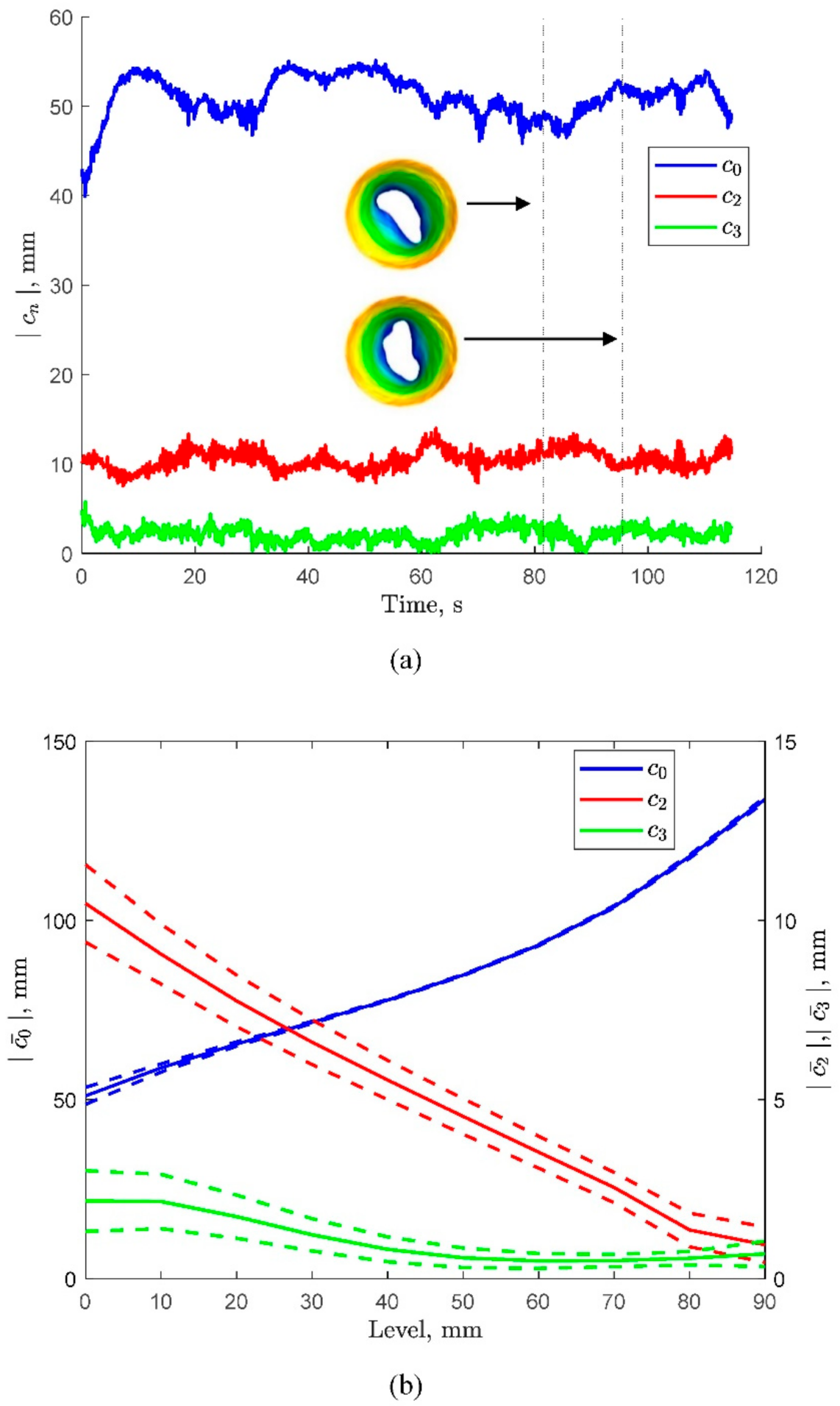
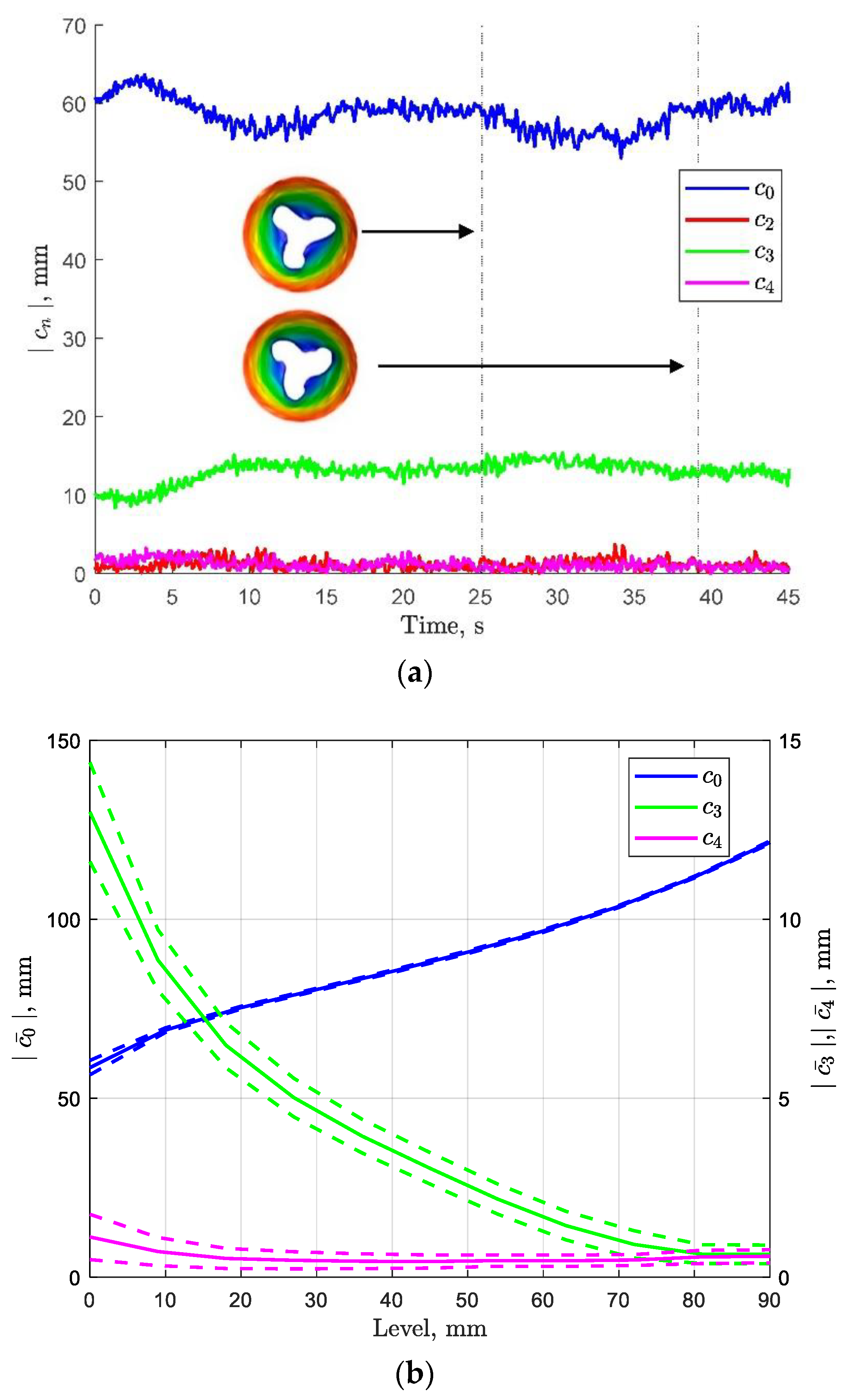
3.2. Pattern Stability
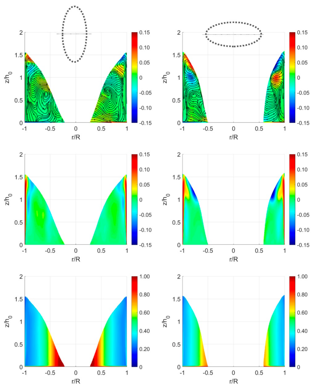
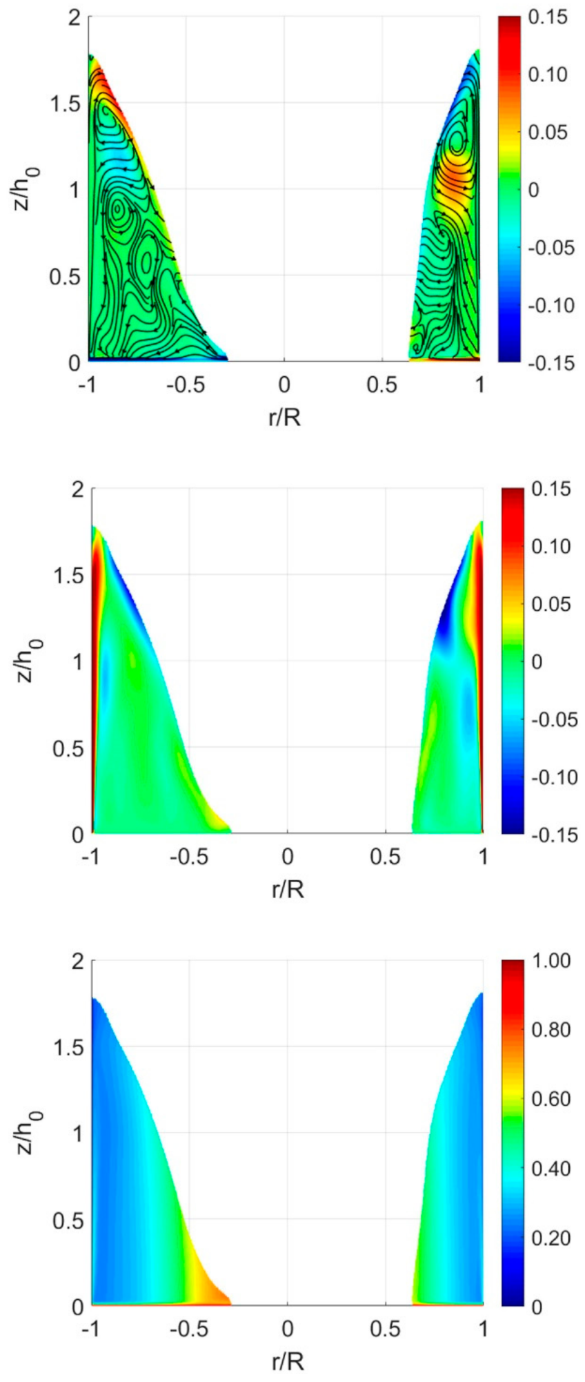
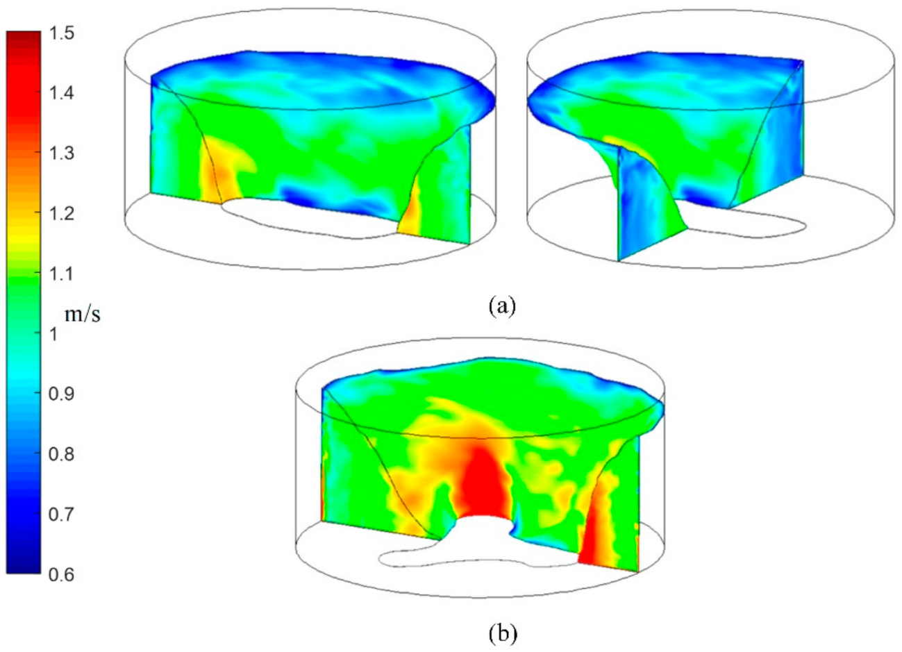
The numerical tool allows obtaining the free surface contours at different heights above the rotating disk. Figure 6 and Figure 7 show the free surface contours at six heights for 3.4 Hz and 4.6 Hz, respectively. For a given height above the disk, the contours as function of time are extracted and rotated to obtain the maximum correlation with the contour at t = 0 (taken arbitrarily). Each contour was plotted on top of the previous ones, forming a color “braid”. The composite contours in Figure 6 and Figure 7 represent the results of combining 1085 contours, which correspond to 108.5 s of computation, and 365 contours (36.5 s of computation), for the frequencies of 3.4 and 4.6 Hz, respectively. It can be seen that ellipses/triangles are getting larger and transform into circles with the increase in the plane height. The “braids” at each height, which contain hundreds of contours, have the same shape after rotation. This shows the stability of the shapes in time. Comparing between the contours at each height, it can be seen that the width of the “braid” of contours decreases with the increase in the height above the cylinder bottom. This shows that raising the height results in more stable shapes. It is also seen, as expected, that the higher the free surface cross-section is taken, the closer to circle shape the contour is, regardless of the underlying shape being ellipse or triangle, eventually converging to a circle with the diameter equal to that of the stationary cylinder (not shown in the figures for brevity).

3.3. Velocity Field

Figure 8 presents top views of radial, axial and normalized tangential average velocities at four heights: 5, 10, 30 and 60 mm, above the disk rotating at 3.4 Hz, where ellipses on the disk surface are observed. Each view is a result of 1085 fields, taken from 108.5 s of computation time. Each field was rotated to best correlate to the t = 0 contour chosen arbitrarily. An average velocity value is shown at a given point if 50% or more frames are occupied by water, otherwise a white color is assigned. This threshold is arbitrary, setting the size of the white “dry spot,” but the mean velocity field around it is captured correctly. In order to expose the velocity field features, the color scales are adjusted to the specific cases, and generally are not kept constant. It can be seen from the left column in Figure 8 that the radial velocity vanishes near the stationary cylinder walls at all the four heights. Closer to the ellipse shape, there are two regions of positive radial velocity and two regions of negative radial velocity. The non-zero velocity regions are positioned such that every apex is surrounded by positive and negative velocity regions. As expected, closer to the rotated disk, the non-zero radial velocities are higher in their absolute values and decrease with height. The maximum absolute radial velocities in the non-zero regions are 0.5, 0.4, 0.2 and 0.1 m/s at 5, 10, 30 and 60 mm above the disk, respectively.
The middle column in Figure 8 presents the average axial velocity at the same four heights. It can be seen that near the stationary walls inside the Stewartson layer the liquid is moving upward with decreasing velocity at greater heights. The upward velocity results from the momentum given to the liquid by the rotating disk in radial direction and the restraint by the stationary cylinder walls. The regions surrounding the ellipse shape are characterized by positive and negative axial velocities. At greater heights the regions of positive velocities become larger at the expense of the negative-velocity regions. The absolute maximum values of axial velocities increase with the increase in height. For example, at 5 mm the maximum value is 0.02 m/s, whereas at 60 mm the velocity is 0.06 m/s. It can be seen from observation of the radial and axial velocities, that near the apex of the ellipse, the liquid is moving radially outward/inward and at the same time upward/downward, correspondingly.
The right column of Figure 8 presents the normalized tangential velocity to highlight the difference between the solid body rotation of the fluid on the rotating disk and the vanishing velocity on the side wall. It can be seen that near the ellipse shape the tangential velocity is approaching the maximum tangential velocity, i.e., the local disk velocity. The tangential velocity of water decreases with radius and vanishes as expected at the stationary cylinder walls. The tangential velocity does not change significantly with height.
Figure 9 presents front cross-sectional views of radial, axial and normalized tangential average velocities. Each view represents averaging of 950 frames which are 95 s of computation. An average velocity value is shown at a given point if 50% or more frames are occupied by water, otherwise a white color is assigned. The velocities at the left column are shown in the vertical plane crossing the water volume through the minor axis of the ellipse, as illustrated at the head of the column. Similarly, the right column represents the velocities in the vertical plane crossing the major axis of the ellipse. It can be seen from the radial velocity distribution and superimposed flow field illustration that the liquid moves radially outward close to the surface of the rotating disk inside the Ekman boundary layer, and then stops at the stationary cylinder. The liquid near the stationary walls is directed upward, as can be seen from the axial velocity, forming a Stewartson boundary layer. The flow is then turning downwards and outward near the surface, as can be seen from the radial and axial velocities. The tangential velocity is getting its local maximum values at the rotating disk and near the axis of rotation; it decreases gradually towards the stationary walls.
Similar to Figure 8, Figure 10 shows the radial, axial and normalized tangential velocities at four heights above the disk rotating at 4.6 Hz. An average velocity value is shown at a given point if 50% or more frames are occupied by water, otherwise a white color is assigned. The computation time is 36.5 s forming 365 datasets. The contours were correlated and rotated as described in the discussion of Figure 8 above. The radial velocity presented in the left column vanishes near the stationary walls for the four heights, similar to Figure 8. However, three regions of non-zero velocities are located aside each triangle arm. Each arm is surrounded by positive and negative radial velocity which decreases with height. For the height of 5 mm, the maximum absolute velocity is 0.5 m/s and for 60 mm the maximum velocity is 0.1 m/s. These radial velocities are similar to the radial velocities obtained for the ellipse shape with 3.4 Hz rotating disk. From the axial velocities in the middle column of Figure 10, it can be seen that the liquid moves upward in a thin layer near the stationary walls and almost remains stationary far from the cylinder walls. However, close to free surface the axial velocity attains both positive and negative values. These regions are located at the same spots around free surface as the non-zero regions of the radial velocity. Thus, it can be observed that the liquid moves inward and downward near each triangle arm and also outward and upward at the other side of each arm. The radial velocity values are quite similar to the ones obtained for the ellipse shape (3.4 Hz) but the axial velocity is higher, reaching values of 0.1 m/s at all heights.
The normalized tangential velocity presented on the right side of Figure 10 shows high values on the valleys of each triangle arm at 5 and 10 mm heights. For all heights, the tangential velocity decreases with radius and does not change significantly with height.
Figure 11 presents front view contours of radial, axial and normalized tangential velocities for three vertical cross-sections positioned 120 degrees from one another. As in Figure 10, each picture is representing averages of 36.5 s of computation time, meaning 365 data sets. From each set, three planes are used for averaging. It can be seen from the contours and superimposed flow field illustration that the fluid is moving radially outward at the rotating disk, then goes up near the stationary walls and moves downward again when approaching the free surface. It is also evident from the tangential velocity distribution that the normalized tangential velocity is higher close to the axis and decreases gradually close to the stationary walls. The tangential velocity does not change significantly with the height. Both Figure 9 and Figure 11 show vortical structures, similar to those attributed to Taylor–Couette flow described in [71]. Secondary flow structures of similar nature were also reported in [72,73].
Figure 12 presents water surface and vertical symmetry plane instantaneous tangential velocity contour maps superimposed onto the water height and rotating bottom disk dry polygon contour lines, for the two shapes observed in the present study: (a) ellipse and (b) triangle. Figure 12a presents the views of two perpendicular planes crossing the water domain along the major (left) and the minor (right) axes of the ellipse, respectively. As can be seen from Figure 12, the water surface angular velocity for the case of ellipse, Figure 12a is almost independent of angular coordinate, showing a marginal increase towards the rotating disk mid-radius, and it decreases further towards the stationary cylinder wall. The same feature is observed also in the trough portion of the triangle polygon, as seen on the right side of Figure 12b. Additionally, as it is seen from Figure 12a, water angular velocity increases towards the ellipse major axis and decreases towards the minor one. This can be attributed to the continuity constraint, as the vertical plane’s effective flow cross-section decreases near the major axis and increases near the minor one, respectively. Similar behavior is observed in Figure 12b for the case of the triangle polygon: the angular velocity intensifies around the triangle polygon crests and decreases towards its troughs.

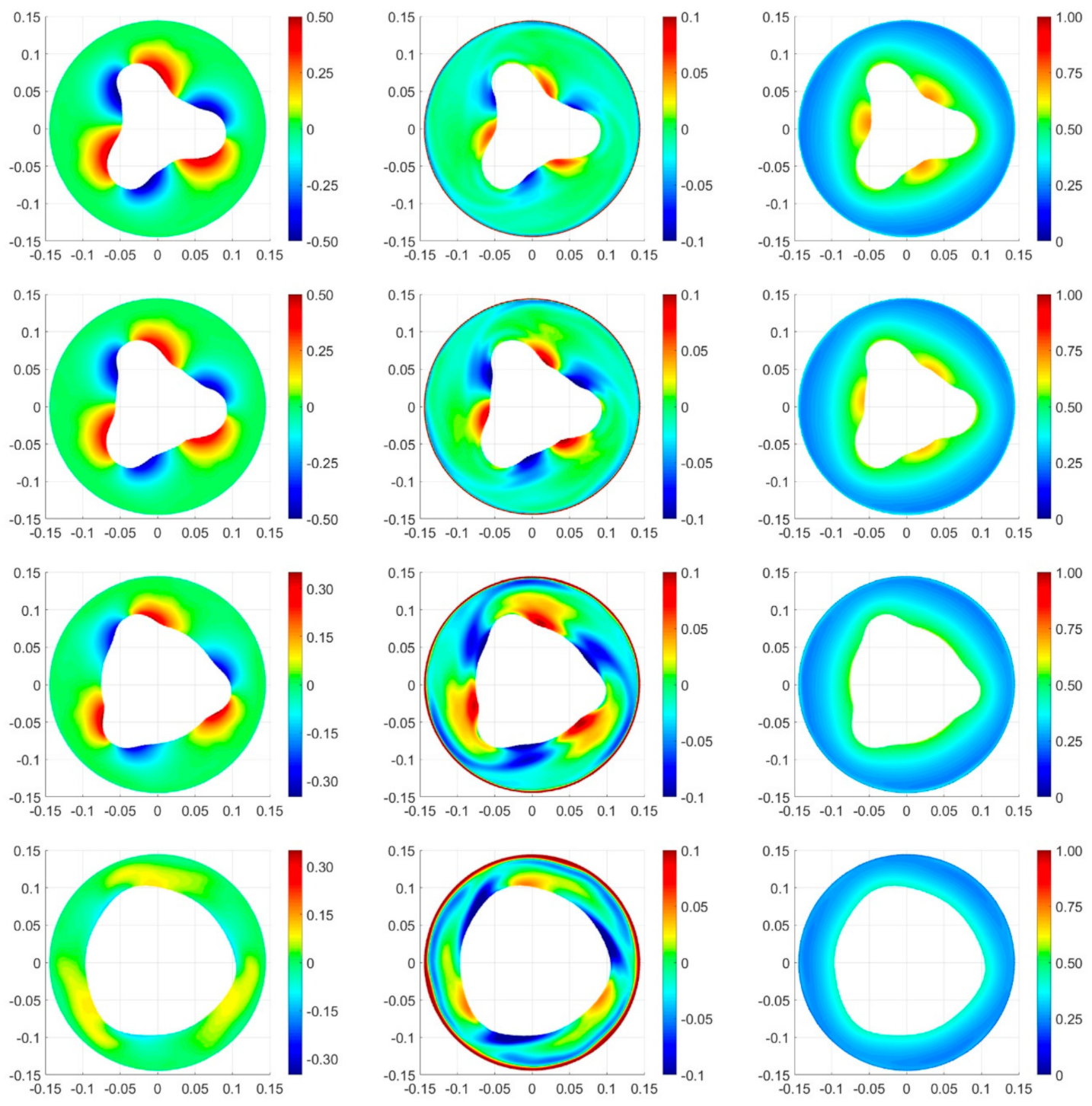
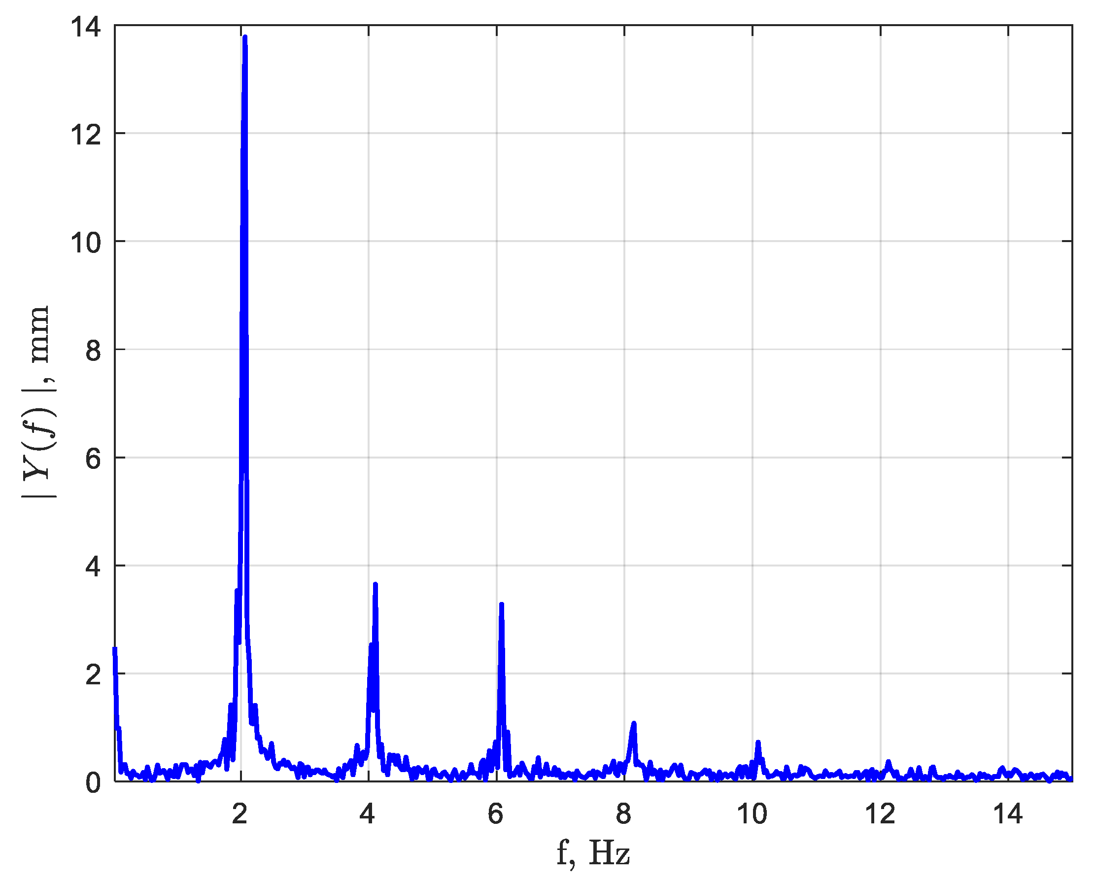
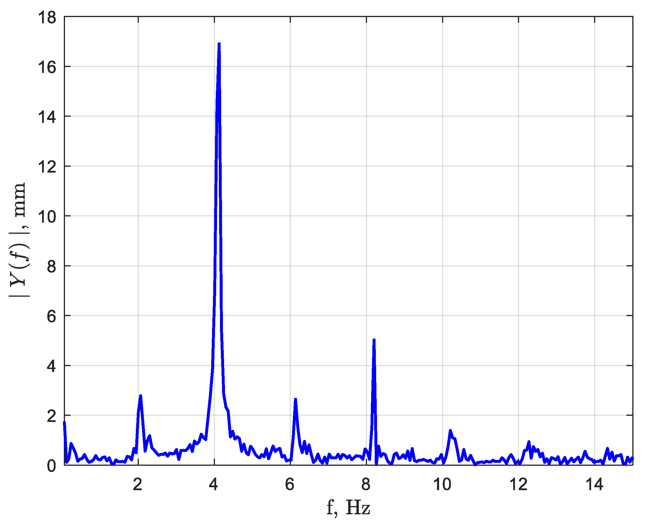
3.4. Fourier Analysis

In addition to the visual representation of Figure 4 and Figure 5, results of Fourier analysis, presented in Figure 13 and Figure 14, enable the identification of the polygon patterns for the frame sequences deduced from the numerical computation. In order to quantify the polygon patterns, a Fourier decomposition is employed, following the procedure of [21]. The contours of the free surface at the level of the rotating disk (zero height) are analyzed by computing their Fourier coefficients as a function of time, where each coefficient corresponds to one polygon pattern expressed by the number of corners, N. The Fourier analysis enables the identification of the dominant pattern at a given instant, and analysis of the stability of the patterns over time. The results are then compared with the frames in Figure 4 and Figure 5 and with the literature.
The polygon rotation frequency is computed for every rotating disk frequency. This is done by analyzing the radius of the free surface contour at the rotating disk level, at one static azimuthal angle as function of time. A Fast Fourier Transform (FFT) is then applied for this function to identify the frequency of the polygon and other features, like the transition between polygon shapes. It is worth noting that in the literature, the polygon frequency measurements were limited to the exposed rotating disk. In the present work, we also computed the frequencies for different heights above the disk, which can be used to quantify the illustrative results of Figure 6 and Figure 7.
The Fourier coefficients c n = 1 2 π 0 2 π r θ e i n θ d θ are computed for the rotating disk frequencies of 3.4 and 4.6 Hz, where r θ is the radius of the free surface contour at the angle θ for selected height. Each coefficient corresponds to a specific polygon pattern. Thus, c0 is the average radius of the polygon; c1 corresponds to the transition of the center of the shape; c2 represents an ellipse and c3 a triangle. In Figure 13 and Figure 14, the dominant and adjacent coefficients are presented for each rotating disk frequency. In order to juxtapose the values of the coefficients and the visual representation of the free surface shapes, Figure 13a and Figure 14a are accompanied with top views at certain times. The dashed lines show the time interval chosen for the free surface level contours presented in Figure 4 and Figure 5.
Figure 13a presents the coefficients c0, c2 and c3 computed at the surface of the 3.4 Hz frequency, as function of time. It can be seen that c0, which corresponds to the average radius of the polygon, is the most dominant coefficient; c2 is the next most dominant coefficient, suggesting that the polygon shape is closer to an ellipse; c3, which corresponds to a triangle, is noticeably smaller than c2. All other coefficients are smaller than c3 and therefore are not presented. The ellipse shapes remain dominant in all computation times. This shows that the ellipse patterns are very stable. The dashed lines show the time interval selected for Figure 4, and first and last figures in Figure 4 are also presented in Figure 13a. Figure 13b shows the dependence of the height on the Fourier coefficients. At each height, the average coefficient in time (solid line) is plotted together with its standard deviation (dashed lines). Since c0 is larger than c2 and c3 by about an order of magnitude, the left vertical axis corresponds to c0 and the right vertical axis corresponds to c2 and c3. It can be seen that as the height above the disk increases, the average radius of the shapes becomes larger and the ellipse coefficient, c2, becomes smaller. This corresponds to the results in Figure 6 where the ellipse transforms into a larger circle when the height increases. In addition, the standard deviations decrease with the height, indicating that the shapes are more stable as the height increases. Accordingly, the widths of the contours (“braids”) in Figure 6 decrease with the height.
Regarding Figure 14a that shows Fourier series coefficients for the rotating disk frequency of 4.6 Hz, it can be seen that the values of c3 become higher than c2. On the other hand, coefficient c4 that corresponds to the next polygon (square) is much smaller than c3, too. This shows quantitatively that the dominant pattern is triangle, as it was shown in Figure 5. In addition, all coefficients remain around their certain values for all computation time. This shows again that the patterns are stable. The dash lines relate Figure 14 to the first and last shapes in Figure 5. Similar to Figure 13b, Figure 14b shows that the shape is getting larger with the height while c3, which is the dominant coefficient (except of course c0), is getting smaller.
The appearance of the two main components of the Fourier series, c0 and c3, obtained numerically in the present study for 4.6 Hz where the triangle polygon shape prevails, was previously reported in [21]—see Figure 4 in that work. The triangle polygon shapes reported in [21] for the initial water height of 40 mm and the rotating disk frequency of 2.4 Hz (Figure 3 in their paper) closely resemble the shapes presented in Figure 5 of the present study. This points at a strong similarity between the triangle shapes obtained experimentally and numerically.
To compute polygon rotation rate, the values of r(θ = 0) at the disk level were stored for each time step of 0.01s, and the FFT was applied to the function. The results in the frequency domain are plotted in Figure 15 and Figure 16, for the disk rotation frequencies of 3.4 Hz and 4.6 Hz, respectively, and at the level of the rotating disk. Only at this height is it possible to compare the present results with the experimental findings from the literature, where image processing was used to compute the rotation rate of the polygons: it was used only on the exposed rotating disk where the contrast between the liquid and the exposed solid surface was large enough, see [10,18,19]. It is worth noting that the numerical calculations are not restricted by this limitation on the image processing.
Figure 15 shows the amplitude Y of each mode for the rotating disk frequency of 3.4 Hz. The largest peak, 2.07, represents the rotation rate of the polygon (ellipse). Since the dominant Fourier coefficient is c2 (see Figure 13), the rotation rate of the polygon is computed by dividing the dominant frequency, 2.07 Hz, by the two polygon “corners” (N = 2), which results in a rotation rate of 1.035 Hz and a ratio of 0.304 between the rotation velocities of the polygon and the disk. The second dominant frequency, 4.11 Hz by the results of Figure 15, corresponds to the next polygon—a triangle. Then, additional peaks, corresponding to higher values of N, are observed. The relative magnitude of the second peak may indicate that the disk rotating frequency is close to a transition between an ellipse and a triangle, as indeed was demonstrated by [10] and can be seen from Figure 3. It may be noted that the computed ratio of frequencies in our case is also close to the value observed by [19].
For the disk frequency of 4.6 Hz, the dominant Fourier coefficient (other than c0) is c3, and its peak frequency from the computation, 4.13 Hz, see Figure 16, should be divided by three, resulting in the ratio of 0.299 between the polygon and the disk rotation velocities. Again, this is very close to the results of [10], where it is reported that the ratios should be within 1/4 to 1/3 [15,19] (see Figure 5 in [19]). It is curious that for the triangular shape, Figure 16, the next peak is smaller than that corresponding to the one at an adjacent higher frequency. It may be speculated that the circles observed in [10], between the triangles and squares, and also maybe those above the squares, are in fact a superposition of a number of polygon shapes. It should be stressed that this study has focused on the ellipse and triangle shapes, hence the higher-order Fourier coefficients (beyond c3) would be explored in a future study.
In fact, the numerical tool allows us to use the same procedure on different heights and not only at the exposed rotating disk as done by the experimental studies. The results show that the polygon frequency as well as the ratio between the dominant frequencies do not change with the height.

4. Conclusions

In the present paper, highly distorted free surface shapes, observed experimentally during the last three decades in liquid flows inside a vertical circular cylinder with a stationary envelope, rotating bottom and open top at the Reynolds numbers of the order of 105, were modeled numerically for the first time in the literature. The parameters and features of this work were chosen based on a scrupulous examination of the existing knowledge, which was extensively presented and analyzed in detail. Accordingly, the cylinder inner radius was 145 mm and the initial water height in it was 60 mm. Following some representative experiments from the literature, bottom disk rotation frequencies of 3.0, 3.4, 4.0 and 4.6 Hz, corresponding to ellipse and triangle shapes, were chosen for the present simulation.
The complexity of the problem in question—highly distorted, turbulent free surface flow—required a carefully chosen combination of state-of-the-art numerical methods. The Large Eddy Simulation (LES) was adopted as the numerical approach, with a localized dynamic Subgrid-Scale Stresses (SGS) model including an energy equation. Since the flow obviously required a surface tracking or capturing method, a volume-of-fluid (VOF) approach was chosen for the present study, based on a careful comparison with the well-known experiments.
The results of the numerical modeling were both extensively visualized and analyzed quantitatively. This was done using radial, axial and tangential velocity fields and average velocity components in different directions. Furthermore, a Fourier analysis was applied to analyze additional features of considerable interest, including the ratio of polygon rotation speed to the bottom rotation speed.
The reported numerical simulations have succeeded to capture all important features of the investigated flow configurations. It was demonstrated that the distorted free surface attained rather distinctive polygon shapes, and that the free surface could become deep enough to expose partially the rotating bottom disk itself, creating “dry” polygons. As expected, the chosen range of geometry and flow parameters included the regions of ellipse and triangle shapes, as observed in the corresponding experimental studies reported in the literature.
The numerical results were found to match the existing experimental observations and measurements, both in terms of the shapes and ranges predicted and in the details of the corresponding flow fields. In most of the simulated cases, the agreement with the existing experimental findings was remarkable. A detailed character of the numerical results allowed for a comprehensive discussion of the underlying physical mechanisms for the characteristic shapes and their transitions. Thus, a unique insight into the free surface flows with rotating polygon shapes was provided.
In our opinion, the significance of the present study goes much beyond the specific type of model flows that it addressed. The reported work presents a considerable step toward better understanding of rotating free surface flows in general. The outcomes of the present investigation indicate that these flows, widely encountered in both nature and engineering systems, can be predicted based on a careful choice of state-of-the-art numerical tools.

Author Contributions

Conceptualization, A.R.; methodology, A.R.; software, U.B.; validation, A.R.; formal analysis, S.D.A.; investigation, A.R. and S.D.A.; writing—original draft preparation, S.D.A.; writing—review and editing, A.R., U.B. and G.Z.; supervision, G.Z.; funding acquisition, A.R. and G.Z. All authors have read and agreed to the published version of the manuscript.

Funding

This research was sponsored by Pazy Foundation.

Institutional Review Board Statement

Not applicable.

Informed Consent Statement

Not applicable.

Data Availability Statement

Not applicable.

Acknowledgments

This study is a part of an ongoing research effort sponsored by Pazy Foundation. The authors would like to express their gratitude to Barak Ostraich for his kind support and assistance in maintaining the computer cluster availability.

Conflicts of Interest

The authors report no conflict of interest.

References

  1. Lugt, H.J. Introduction to Vortex Theory; Vortex Flow Press: Potomac, MD, USA, 1996. [Google Scholar]
  2. Childs, P.R.N. Rotating Flows; Butterworth-Heinemann (Elsevier): Oxford, UK, 2011. [Google Scholar]
  3. Andersen, A.; Bohr, T.; Stenum, B.; Rasmussen, J.J.; Lautrup, B. The bathtub vortex in a rotating container. J. Fluid Mech. 2006, 556, 121–146. [Google Scholar] [CrossRef] [Green Version]
  4. Vatistas, G.H. A note on liquid vortex sloshing and Kelvin’s equilibria. J. Fluid Mech. 1990, 217, 241–248. [Google Scholar] [CrossRef]
  5. Kelvin, L. Vibrations of a columnar vortex. Philos. Mag. 1880, 10, 155–168. [Google Scholar]
  6. Vatistas, G.H.; Wang, J.; Lin, S. Experiments on waves induced in the hollow core of vortices. Exp. Fluids 1992, 13, 377–385. [Google Scholar] [CrossRef]
  7. Jansson, T.R.N.; Haspang, M.P.; Jensen, K.H.; Hersen, P.; Bohr, T. Polygons on a rotating fluid surface. Phys. Rev. Lett. 2006, 96, 174502. [Google Scholar] [CrossRef] [Green Version]
  8. Suzuki, T.; Iima, M.; Hayase, Y. Surface switching of rotating fluid in a cylinder. Phys. Fluids 2006, 18, 101701. [Google Scholar] [CrossRef]
  9. Poncet, S.; Chauve, M.P. Shear-layer instability in a rotating system. J. Flow Vis. Image Process. 2007, 14, 85–105. [Google Scholar] [CrossRef]
  10. Bach, B.; Linnartz, E.C.; Vested, M.H.; Andersen, A.; Bohr, T. From Newton’s bucket to rotating polygons: Experiments on surface instabilities in swirling flows. J. Fluid Mech. 2014, 759, 386–403. [Google Scholar] [CrossRef]
  11. Abderrahmane, H.A.; Fayed, M.; Ng, H.D.; Vatistas, G.H. Synchronization of traveling waves within a hollow-core vortex. IJMEM 2017, 11, 742–746. [Google Scholar]
  12. Vatistas, G.H. Comment on “Surface switching of rotating fluid in a cylinder” [Phys. Fluids 18, 101701 (2006)]. Phys. Fluids 2007, 19, 069101. [Google Scholar] [CrossRef] [Green Version]
  13. Tasaka, Y.; Ito, K.; Iima, M. Visualization of a rotating flow under large-deformed free surface using anisotropic flakes. J. Vis. 2008, 11, 163–172. [Google Scholar] [CrossRef]
  14. Tasaka, Y.; Iima, M. Flow transitions in the surface switching of rotating fluid. J. Fluid Mech. 2009, 636, 475–484. [Google Scholar] [CrossRef] [Green Version]
  15. Vatistas, G.H.; Abderrahmane, H.A.; Siddiqui, M.H.K. Experimental confirmation of Kelvin’s equilibria. Phys. Rev. Lett. 2008, 100, 174503. [Google Scholar] [CrossRef]
  16. Thomson, J.J. A Treatise on the Motion of Vortex Rings—An Essay to Which the Adams Prize Was Adjudged in 1882, in the University of Cambridge; Macmillan: London, UK, 1883. [Google Scholar]
  17. Havelock, T.H. LII. The stability of motion of rectilinear vortices in ring formation. Lond. Edinb. Dublin Philos. Mag. J. Sci. 1931, 7, 617–633. [Google Scholar] [CrossRef]
  18. Abderrahamne, H.A.; Siddiqui, K.; Vatistas, G.H. Transition between Kelvin’s equilibria. Phys. Rev. E 2009, 80, 066305. [Google Scholar] [CrossRef]
  19. Abderrahmane, H.A.; Siddiqui, K.; Vatistas, G.H. Rotating waves within a hollow vortex core. Exp. Fluids 2011, 50, 677–688. [Google Scholar] [CrossRef]
  20. Abderrahmane, H.A.; Siddiqui, K.; Vatistas, G.H.; Fayed, M.; Ng, H.D. Symmetrization of a polygonal hollow-core vortex through beat-wave resonance. Phys. Rev. E 2011, 83, 056319. [Google Scholar] [CrossRef] [PubMed] [Green Version]
  21. Bergmann, R.P.H.M.; Tophøj, L.; Homan, T.A.M.; Hersen, P.; Andersen, A.; Bohr, T. Polygon formation and surface flow on a rotating fluid surface. J. Fluid Mech. 2011, 679, 415, Erratum in 2012, 691, 605. [Google Scholar] [CrossRef] [Green Version]
  22. Abderrahmane, H.A.; Fayed, M.; Ng, H.D.; Vatistas, G.H. A note on relative equilibria in a rotating shallow water layer. J. Fluid Mech. 2013, 724, 695–703. [Google Scholar] [CrossRef] [Green Version]
  23. Iga, K.; Yokota, S.; Watanabe, S.; Ikeda, T.; Niino, H.; Misawa, N. Various phenomena on a water vortex in a cylindrical tank over a rotating bottom. Fluid Dyn. Res. 2014, 46, 031409. [Google Scholar] [CrossRef]
  24. Abderrahmane, H.A.; Fayed, M.; Ng, H.D.; Vatistas, G.H. New experimental confirmation of Kelvin’s equilibria. Eur. Phys. J. Plus 2018, 133, 339. [Google Scholar] [CrossRef]
  25. Jansson, T.R.N.; Haspang, M.P.; Jensen, K.H. Symmetry Breaking in the Free Surface of Rotating Fluids with High Reynolds Numbers. Bachelor’s Project, University of Copenhagen, Copenhagen, Denmark, December 2004. [Google Scholar]
  26. Vatistas, G.H.; Wang, J.; Lin, S. Recent findings on Kelvin’s equilibria. ACTA Mech. 1994, 103, 89–102. [Google Scholar] [CrossRef]
  27. Tophoj, L.; Mougel, J.; Bohr, T.; Fabre, D. Rotating polygon instability of a swirling free surface flow. Phys. Rev. Lett. 2013, 110, 194502. [Google Scholar] [CrossRef] [PubMed] [Green Version]
  28. Iima, M.; Tasaka, Y. Dynamics of flow structures and surface shapes in the surface switching of rotating fluid. J. Fluid Mech. 2016, 789, 402–424. [Google Scholar] [CrossRef] [Green Version]
  29. Fabre, D.; Mougel, J. Generation of three-dimensional patterns through wave interaction in a model of free surface swirling flow. Fluid Dyn. Res. 2014, 46, 061415. [Google Scholar] [CrossRef]
  30. Amaouche, M.; Abderrahmane, H.A.; Vatistas, G.H. Nonlinear modes in the hollow-cores of liquid vortices. Eur. J. Mech. B/Fluids 2013, 41, 133–137. [Google Scholar] [CrossRef]
  31. Yellin-Bergovoy, R.; Heifetz, E.; Umurhan, O.M. Physical mechanism of centrifugal-gravity wave resonant instability in azimuthally symmetric swirling flows. Phys. Rev. Fluids 2017, 2, 104801. [Google Scholar] [CrossRef]
  32. Mougel, J.; Fabre, D.; Lacaze, L.; Bohr, T. On the instabilities of a potential vortex with a free surface. J. Fluid Mech. 2017, 824, 230–264. [Google Scholar] [CrossRef] [Green Version]
  33. Spohn, A.; Mory, M.; Hopfinger, E.J. Observations of vortex breakdown in an open with a rotating bottom. Exp. Fluids 1993, 14, 70–77. [Google Scholar] [CrossRef]
  34. Brøns, M.; Voigt, L.K.; Sørensen, J.N. Topology of vortex breakdown bubbles in a cylinder with a rotating bottom and a free surface. J. Fluid Mech. 2001, 428, 133–148. [Google Scholar] [CrossRef]
  35. Bouffanais, R.; Jacono, D.L. Transitional cylindrical swirling flow in presence of a flat free surface. Comput. Fluids 2009, 38, 1651–1673. [Google Scholar] [CrossRef] [Green Version]
  36. Bouffanais, R.; Jacono, D.L. Unsteady transitional swirling flow in the presence of a moving free surface. Phys. Fluids 2009, 21, 64107. [Google Scholar] [CrossRef] [Green Version]
  37. Miraghaie, R.; Lopez, J.M.; Hirsa, A.H. Flow induced patterning at the air–water interface. Phys. Fluids 2003, 15, L45. [Google Scholar] [CrossRef] [Green Version]
  38. Lopez, J.M.; Marques, F.; Hirsa, A.H.; Miraghaie, R. Symmetry breaking in free-surface cylinder flows. J. Fluid Mech. 2004, 502, 99–126. [Google Scholar] [CrossRef] [Green Version]
  39. Valentine, D.T.; Jahnke, C.C. Flows induced in a cylinder with both end walls rotating. Phys. Fluids 1994, 6, 2702–2710. [Google Scholar] [CrossRef]
  40. Lopez, J.M. Unsteady swirling flow in an enclosed cylinder with reflectional symmetry. Phys. Fluids 1995, 7, 2700–2714. [Google Scholar] [CrossRef] [Green Version]
  41. Gelfgat, A.; Bar-Yoseph, P.Z.; Solan, A. Three-dimensional instability of axisymmetric flow in a rotating lid–cylinder enclosure. J. Fluid Mech. 2001, 438, 363–377. [Google Scholar] [CrossRef] [Green Version]
  42. Marques, F.; Lopez, J.M. Precessing vortex breakdown mode in an enclosed cylinder flow. Phys. Fluids 2001, 13, 1679–1682. [Google Scholar] [CrossRef] [Green Version]
  43. Poncet, S. The stability of a thin water layer over a rotating disk revisited. Eur. Phys. J. Plus 2014, 129, 167. [Google Scholar] [CrossRef]
  44. Kahouadji, L. Analyse de Stabilité Linéaire D’écoulements Tournants en Présence de Surface Libre. Ph.D. Thesis, Université Pierre et Marie Curie, Paris, France, 2011. [Google Scholar]
  45. Niino, H.; Misawa, N. An Experimental and theoretical study of barotropic instability. J. Atmos. Sci. 1984, 41, 1992–2011. [Google Scholar] [CrossRef] [Green Version]
  46. Kahouadji, L.; Witkowski, L.M. Free surface due to a flow driven by a rotating disk inside a vertical cylindrical tank: Axisymmetric configuration. Phys. Fluids 2014, 26, 072105. [Google Scholar] [CrossRef] [Green Version]
  47. Piva, M.; Meiburg, E. Steady axisymmetric flow in an open cylindrical container with a partially rotating bottom wall. Phys. Fluids 2005, 17, 063603. [Google Scholar] [CrossRef]
  48. Yang, W.; Delbende, I.; Fraigneau, Y.; Witkowski, L.M. Axisymmetric rotating flow with free surface in a cylindrical tank. J. Fluid Mech. 2018, 861, 796–814. [Google Scholar] [CrossRef] [Green Version]
  49. Iga, K. Axisymmetric flow in a cylindrical tank over a rotating bottom. Part I. Analysis of boundary layers and vertical circulation. Fluid Dyn. Res. 2017, 49, 065502. [Google Scholar] [CrossRef]
  50. Iga, K.; Yokota, S.; Watanabe, S.-I.I.; Ikeda, T.; Niino, H.; Misawa, N. Axisymmetric flow in a cylindrical tank over a rotating bottom. Part II. Deformation of the water surface and experimental verification of the theory. Fluid Dyn. Res. 2017, 49, 065501. [Google Scholar] [CrossRef] [Green Version]
  51. Ansys® Fluent, Release 19.0.0; ANSYS Inc.: Canonsburg, PA, USA, 2019.
  52. Silva, M.F.; Campos, J.B.L.M.; Miranda, J.M.; Araújo, J.D.P. Numerical study of single Taylor bubble movement through a microchannel using different CFD packages. Processes 2020, 8, 1418. [Google Scholar] [CrossRef]
  53. Sagaut, P. Large Eddy Simulation for Incompressible Flows: An Introduction, 3rd ed.; Springer: Berlin/Heidelberg, Germany, 2005. [Google Scholar]
  54. Kim, W.W.; Menon, S. An unsteady incompressible Navier–Stokes solver for large eddy simulation of turbulent flows. Int. J. Numer. Methods Fluids 1999, 31, 983–1017. [Google Scholar] [CrossRef]
  55. Pallares, J.; Davidson, L. Large-eddy simulations of turbulent flow in a rotating square duct. Phys. Fluids 2000, 12, 2878. [Google Scholar] [CrossRef]
  56. McSherry, R.J.; Chua, K.V.; Stoesser, T. Large eddy simulation of free-surface flows. J. Hydrodyn. 2017, 29, 1–12. [Google Scholar] [CrossRef]
  57. Hirt, C.; Nichols, B. Volume of fluid (VOF) method for the dynamics of free boundaries. J. Comput. Phys. 1981, 39, 201–225. [Google Scholar] [CrossRef]
  58. Osher, S.; Sethian, J.A. Fronts propagating with curvature-dependent speed: Algorithms based on Hamilton-Jacobi formulations. J. Comput. Phys. 1988, 79, 12–49. [Google Scholar] [CrossRef] [Green Version]
  59. Gopala, V.R.; van Wachem, B.G. Volume of fluid methods for immiscible-fluid and free-surface flows. Chem. Eng. J. 2008, 141, 204–221. [Google Scholar] [CrossRef]
  60. Sethian, J.A.; Smereka, P. Level set methods for fluid interfaces. Annu. Rev. Fluid Mech. 2003, 35, 341–372. [Google Scholar] [CrossRef] [Green Version]
  61. Yue, W.; Lin, C.-L.; Patel, V.C. Large eddy simulation of turbulent open-channel flow with free surface simulated by level set method. Phys. Fluids 2005, 17, 25108. [Google Scholar] [CrossRef]
  62. Suh, J.; Yang, J.; Stern, F. The effect of air–water interface on the vortex shedding from a vertical circular cylinder. J. Fluids Struct. 2011, 27, 1–22. [Google Scholar] [CrossRef]
  63. Sussman, M.; Puckett, E.G. A coupled level set and volume-of-fluid method for computing 3D and axisymmetric incompressible two-phase flows. J. Comput. Phys. 2000, 162, 301–337. [Google Scholar] [CrossRef] [Green Version]
  64. Zi, D.; Xuan, A.; Wang, F.; Shen, L. Numerical study of mechanisms of air-core vortex evolution in an intake flow. Int. J. Heat Fluid Flow 2020, 81, 108517. [Google Scholar] [CrossRef]
  65. Stachnik, M.; Jakubowski, M. Multiphase model of flow and separation phases in a whirlpool: Advanced simulation and phenomena visualization approach. J. Food Eng. 2020, 274, 109846. [Google Scholar] [CrossRef]
  66. McCraney, J.; Weislogel, M.; Steen, P. OpenFOAM Simulations of late stage container draining in microgravity. Fluids 2020, 5, 207. [Google Scholar] [CrossRef]
  67. Tembely, M.; Alameri, W.S.; Alsumaiti, A.M.; Jouini, M.S. Pore-scale modeling of the effect of wettability on two-phase flow properties for newtonian and non-newtonian fluids. Polymers 2020, 12, 2832. [Google Scholar] [CrossRef]
  68. Celik, I.B.; Cehreli, Z.N.; Yavuz, I. Index of resolution quality for large eddy simulations. J. Fluids Eng. 2005, 127, 949–958. [Google Scholar] [CrossRef]
  69. Klein, M.; Meyers, J.; Geurts, B.J. Assessment of LES quality measures using the error landscape approach. In Direct and Large-Eddy Simulation VII; Springer Nature: Berlin/Heidelberg, Germany, 2008; Volume 12, pp. 131–142. [Google Scholar]
  70. Pope, S.B. Turbulent Flows. Meas. Sci. Technol. 2001, 12, 2020–2021. [Google Scholar] [CrossRef]
  71. Mulligan, S.; De Cesare, G.; Casserly, J.; Sherlock, R. Understanding turbulent free-surface vortex flows using a Taylor-Couette flow analogy. Sci. Rep. 2018, 8, 824. [Google Scholar] [CrossRef] [PubMed] [Green Version]
  72. Jakubowski, M.; Diakun, J. Simulation investigations of the effects of whirlpool dimensional ratios on the state of secondary whirls. J. Food Eng. 2007, 83, 106–110. [Google Scholar] [CrossRef]
  73. Jakubowski, M.; Wyczalkowski, W.; Poreda, A. Flow in a symmetrically filled whirlpool: CFD modelling and experimental study based on Particle Image Velocimetry (PIV). J. Food Eng. 2015, 145, 64–72. [Google Scholar] [CrossRef]
Figure 1. The system addressed in the present study: (a) physical model and an example of a polygon created on the disk surface; (b) computational domain and grid (front and top views).
Applsci 11 01348 g001
Figure 2. Evaluation of Large Eddy Simulation (LES) quality for a typical instant flow field: (a) LES index of quality (LESIQν) for a free distorted surface shown in top view; (b) LESIQν for a vertical cross-section of the same flow field; (c) the Courant number for the same cross-section.
Applsci 11 01348 g002
Figure 3. Circumferentially and time-averaged water height, simulated in the present study, vs. measurements from the literature.
Applsci 11 01348 g003
Figure 4. Top view of the free surface height above rotating disk for 3.4 Hz, from top left to bottom right, equally spaced within about 14 s of computation.
Applsci 11 01348 g004
Figure 5. Top view contours of the free surface height above rotating disk for its rotation frequency of 4.6 Hz, from top left to bottom right, equally spaced within 14 s of computation.
Applsci 11 01348 g005
Figure 6. Free surface contours at six heights for 3.4 Hz disk rotation frequency. Each contour is rotated to the contour of t = 0 s using maximum correlation between the shapes. For each height 1085 contours are plotted representing results for 108.5 s.
Applsci 11 01348 g006
Figure 7. Free surface contours at six levels for 4.6 Hz disk rotation frequency. Each contour is rotated to the contour of t = 0 s using maximum correlation between the shapes. For each height 360 contours are plotted, representing results for 36 s.
Applsci 11 01348 g007
Figure 8. Top view of the radial, axial (both in m/s) and normalized tangential average velocities at four heights (from top to bottom: 5, 10, 30 and 60 mm) above the 3.4 Hz rotating disk. Each contour is rotated to the contour of t = 0 s using maximum correlation between the shapes. Velocity values are averaged if the specific location was occupied by water more than 50% of the frames, otherwise white color is assigned.
Applsci 11 01348 g008
Figure 9. Front view contours of the radial, axial (both in m/s) and normalized tangential velocities in the two vertical cross-sections corresponding to the main axes of the ellipse at the disk rotation frequency of 3.4 Hz. Each velocity field is averaged over 950 frames which represent 95 s of a transient.
Applsci 11 01348 g009
Figure 10. Top view contours of the radial, axial (both in m/s) and normalized tangential velocities at four heights (from top to bottom: 5, 10, 30 and 60 mm) above the 4.6 Hz rotating disk. Each contour is rotated to the contour of t = 0 s using maximum correlation between the shapes. Velocity values are averaged if the specific location was occupied by water more than 50% of the frames, otherwise white color is assigned.
Applsci 11 01348 g010
Figure 11. Front view contours of the radial, axial (both in m/s) and normalized tangential velocities for the vertical cross-section of the triangle, at the at the disk rotation frequency of 4.6 Hz. Each picture represents averaging of 1095 planes which are taken over the time span of 36.5 s (3 planes for every 0.1 s).
Applsci 11 01348 g011
Figure 12. Instantaneous tangential velocity contours: (a) elliptical polygon for 3.4 Hz, (b) triangular polygon for 4.6 Hz.
Applsci 11 01348 g012
Figure 13. The Fourier coefficients, c0 to c3 for 3.4 Hz rotating disk frequency: (a) the Fourier coefficients as function of time at the surface of the rotating disk. (b) The average and standard deviation of the Fourier coefficients for the time interval presented in (a) at different heights above the rotating disk. The left vertical axis corresponds to c0 and the right vertical axis corresponds to c2 and c3.
Applsci 11 01348 g013
Figure 14. The Fourier coefficients, c0 to c4, for 4.6 Hz rotating disk frequency: (a) the Fourier coefficients as function of time at the surface of the rotating disk. (b) The average and standard deviation of the Fourier coefficients for the time interval presented in (a) at different heights above the rotating disk. The left vertical axis corresponds to c0 and the right vertical axis corresponds to c2 and c3.
Applsci 11 01348 g014
Figure 15. Fourier transform for rotating disk frequency of 3.4 Hz.
Applsci 11 01348 g015
Figure 16. Fourier transform for rotating disk frequency of 4.6 Hz.
Applsci 11 01348 g016
Table 1. Previous experiments and present study: parameters and dimensionless numbers.
r
mm
R
mm
h
mm
ω
rad/s
ν × 106
m2/s
Re = ωr2/νFr = ωr/(gh)0.5h/Rr/RDetectable Polygons—N
Vatistas [4]126142.515025.11 a3.99 × 1052.611.050.88No, periodic sloshing without surface exposed
126142.529381.71.30 × 1066.072.060–2, periodic sloshing with surface exposed from circular to elliptical cross section
101 a142.56310.5–31.41.07 × 105–3.20 × 1051.35–4.040.44 0.710–6
691.29–3.860.480–5
Vatistas et al. [6]12614224, 275.2–25.118.31 × 104–4.16 × 1051.28–6.800.17–0.190.890–6
518.8–31.456.75.28 × 103–8.80 × 10310.72–17.870.045–11
715.7–25.14.40 × 103–7.04 × 1037.55–12.080.055–10
1019.9–30.45.57 × 103–8.50 × 1038.00–12.220.074–8
2215.7–27.24.40 × 103–1.09 × 1050.61–7.380.150–8
>100>83.8640>2.08 × 10³>10.660.700
Jansson et al. [7] 144 b145b25–1003.1–44.01 c6.51 × 104–9.12 × 1050.46–12.790.17–0.690.990–6
154.34 × 10³–6.08 × 1040–3
19319425–953.1–31.41 c1.17 × 105–1.17 × 1060.61–12.240.13–0.520–5
Suzuki et al. [8]4242.540<146.41<2.58 × 10⁵<9.82 0.940.990–2, surface exposed from circular to elliptical cross sections
Poncet and Chauve [9]140140.85 ± 0.052.5–150–6.21≤1.21 × 1052.25–5.52≤0.110.990–8 without 2
Bach et al. [10]14414530-802.5–40.815.21 × 104 – 8.47 × 1050.41–10.480.21–0.550.990-5
Ait Abderrahmane et al. [11]14014220, 30, 407.9–28.01-22 d7.00 × 103–5.48 × 1051.76–8.840.14–0.280.990–6
Present study1451456018.8, 21.4, 25.1, 28.913.96 × 105–6.08 × 1053.56–5.460.4110–3
a Value not specified exactly in the text. The disk radius was obtained from [10]. b Obtained from [10] with the same experimental set-up. c Value not specified exactly in the text. d Under the assumption of equal density to water.
Publisher’s Note: MDPI stays neutral with regard to jurisdictional claims in published maps and institutional affiliations.

