Binary Spring Search Algorithm for Solving Various Optimization Problems

Abstract

One of the most powerful tools for solving optimization problems is optimization algorithms (inspired by nature) based on populations. These algorithms provide a solution to a problem by randomly searching in the search space. The design’s central idea is derived from various natural phenomena, the behavior and living conditions of living organisms, laws of physics, etc. A new population-based optimization algorithm called the Binary Spring Search Algorithm (BSSA) is introduced to solve optimization problems. BSSA is an algorithm based on a simulation of the famous Hooke’s law (physics) for the traditional weights and springs system. In this proposal, the population comprises weights that are connected by unique springs. The mathematical modeling of the proposed algorithm is presented to be used to achieve solutions to optimization problems. The results were thoroughly validated in different unimodal and multimodal functions; additionally, the BSSA was compared with high-performance algorithms: binary grasshopper optimization algorithm, binary dragonfly algorithm, binary bat algorithm, binary gravitational search algorithm, binary particle swarm optimization, and binary genetic algorithm. The results show the superiority of the BSSA. The results of the Friedman test corroborate that the BSSA is more competitive.

1. Introduction

The optimization of a process or system is a concept that has critical applications in many fields of science. Many optimization algorithms have been introduced [1,2,3], which has led to greater availability of heuristic optimization techniques in recent years and their application in various fields, such as energy [4,5], protection [6], electrical engineering [7,8,9,10,11], filter design [12], and energy carriers [13,14], to achieve the optimal solution (under specific criteria). Lately, these methods have been modified, achieving better yields [15,16,17].

An optimization algorithm is intelligent when its approach is to find an adequate solution to an optimization problem in the shortest possible time with the least detailed information [18]. The word “heuristics” in ancient Greek means “to know,” “to discover,” “to find,” or “a clue for an investigation” [19]. The heuristic approach ignores some of the information to make faster decisions with the maximum saving of time and utmost precision compared to complex approaches [20]. Processes in nature inspire many heuristic algorithms (biological processes, animals or groups of animals, and physics theories).

Optimization algorithms can be classified in different ways, using a widely accepted structure of four categories, based on the main design. These categories are physics-based, swarm, game-based, and evolution-based optimization algorithms.

Physics-based optimization algorithms are designed according to the simulation of various phenomena and laws of physics. Momentum Search Algorithm (MSA) is one of the algorithms belonging to this group. MSA is based on the simulation of momentum and motion laws. Members of the MSA population are balls with different weights that move in the direction of a ball with a suitable position based on the impulse [1]. Simulated Annealing (SA) algorithm is one of the oldest algorithms in physics. SA is inspired by the process of smelting and cooling materials in metallurgy. Under controlled temperature conditions, the materials are subjected to a heat treatment that causes the molecular structures to go through different phases to change their mechanical properties. The previous phenomenon increases the strength and durability of the material. Heating the material increases its atoms’ energy. It allows them to move freely, and the slow cooling process allows a new, lower-energy, higher-strength configuration to be discovered and exploited [21]. This algorithm’s efficiency is due to an essential connection between statistical mechanics and optimization processes (multivariate or combinatorial in nature).

The analogous behavior of these processes lays the foundations for defining values that optimize the properties of extensive and/or complex systems, which is where the use of this algorithm is mainly justified.

Some other popular physics-based optimization algorithms include Galaxy-based Search Algorithm (GbSA) [22], Charged System Search (CSS) [23], Curved Space Optimization (CSO) [24], Artificial Chemical Reaction Optimization Algorithm (ACROA) [25], Ray Optimization (RO) algorithm [26], Small World Optimization Algorithm (SWOA) [27], Black Hole (BH) [28], Central Force Optimization (CFO) [29], and Big-Bang Big-Crunch (BBBC) [30].

Swarm-based optimization algorithms have been developed based on the simulation of natural processes, movements, and behavior of animals and other living things. Particle Swarm Optimization (PSO) is the most famous optimization algorithm and is often used by researchers. Particle swarm optimization is a heuristic global optimization method that was proposed in 1995 [31]. It is based on the intelligence of swarms and emulates the behavior patterns of birds/fish when looking for food. One of the birds smells food and communicates it to the rest; this coordination reproduces successful behavior due to the cooperation of each bird. This algorithmically structured idea, due to its simplicity and ease of implementation, is widely exploited for optimization in many different areas of knowledge.

Some of the other swarm-based algorithms are Bat-inspired Algorithm (BA) [32], Artificial Bee Colony (ABC) [33], Doctor and Patient Optimization (DPO) [34], Cuckoo Search (CS) [35], Spotted Hyena Optimizer (SHO) [36], Multi Leader Optimizer (MLO) [37], Group Optimization (GO) [38], Monkey Search (MS) [39], Grey Wolf Optimizer (GWO) [40], Artificial Fish-Swarm Algorithm (AFSA) [41], Hunting Search (HS) [42], Moth-Flame Optimization Algorithm (MFO) [43], Emperor Penguin Optimizer (EPO) [44], Dolphin Partner Optimization (DPO) [45], Donkey Theorem Optimization (DTO) [46], Rat Swarm Optimizer (RSO) [47], Grasshopper Optimization Algorithm (GOA) [48], Coupled Spring Forced Bat Algorithm (SFBA) [49], and Following Optimization Algorithm (FOA) [50].

Game-based optimization algorithms are introduced and designed based on the simulation of different game rules and player behavior. Football Game-Based Optimization (FGBO) is a game-based optimization algorithm developed based on football league simulations and club performance [51]. Some of the other game-based algorithms are Binary Orientation Search Algorithm (BOSA) [52], Darts Game Optimizer (DGO) [53], Orientation Search Algorithm (OSA) [54], Shell Game Optimization (SGO) [55], Dice Game Optimizer (DGO) [56], and Hide Objects Game Optimization (HOGO) [57].

Evolutionary-based optimization algorithms are developed based on the combination of natural selection and continuity of coordination. These algorithms are based on structures that simulate the rules of selection, recombination, change, and survival. Genetic Algorithm (GA) is one of the oldest and most popular evolutionary-based optimization algorithms [58]. Some other evolutionary-based algorithms include Improved Quantum-Inspired Differential Evolution Algorithm (IQDE) [59], Differential Evolution (DE) [60], Biogeography-Based Optimizer (BBO) [61], Evolutionary Programming (EP) [62], Evolution Strategy (ES) [63], and Genetic Programming (GP) [64].

These algorithms use a kind of statistical feature and random phenomena in their structure. Some central force optimization algorithms that are metaphors for the global law of gravity do not use such random phenomena. Such algorithms have certainty characteristics [29].

Population-based approaches have been inspired by social interactions between members of a community.

Based on the experience learned and the neighborhood particle guides, every particle tries to move towards the search space’s best position [65]. Physical and biological processes and nature have inspired heuristic search algorithms. The majority of them act as population-based algorithms.

Unlike classical techniques, heuristic search techniques act randomly and search space in parallel; they do not use spatial gradient information. These algorithms use only fitness functions to guide the search process, but they can discover the solution thanks to their swarm intelligence. Swarm intelligence appears in cases where there is a population of non-expert factors. These factors have a simple behavior/pattern in certain situations/conditions and interact locally. These localized relationships/interactions between members cause unexpected ultralocal interactions and guide the search to the optimal solution. This allows the system/process to find a solution without the need for a central controller. The members’ behavior/performance organizes the system internally, generating characteristics such as positive feedback, negative feedback, balanced exploration-exploitation, and multiple interactions of a different order. This effect is called the self-organizing impact [66,67].

Although heuristic algorithms have been developed, improved, and used, no algorithm has been introduced that provides an efficient solution for optimizing engineering problems or problems in other sciences. This article analyzes/discusses a new heuristic algorithm that solves the traditional shortcomings. An optimization algorithm based on the well-known Hooke’s law is proposed, and preliminary results are presented [68].

The optimization algorithm called Binary Spring Search Algorithm (BSSA) is described and analyzed. The rest of the paper is organized as follows. In the first section, a brief introduction to heuristic-based optimization algorithms is presented. The spring force law is discussed in the second section, and the binary version of the spring search algorithm is introduced in Section 3. The main features of the BBSA are shown in Section 4, and a computational complexity analysis is presented in Section 5. The proposed algorithm’s exploration and exploitation characteristics are explained in Section 6, and the results are given in Section 7. Finally, concluding remarks are listed in the last section.

2. Spring Search Algorithm

The BSSA is a physics-based optimization algorithm that can be used to solve various optimization problems. The BSSA has a population matrix whose members are different weights that are moved in the search space in order to achieve the optimal solution. All desired weights are connected to each other in this system by a unique spring whose stiffness coefficient is determined based on the value of the objective function. The main idea of the proposed BSSA is to use Hooke’s law between the weights and springs in order to reach the equilibrium point (solution).

Hooke’s law is defined using Equation (1). All springs follow Hooke’s law as long as they are not deformed [69].

$$F_s=-kx$$

(1)

Here, $F_s$ is the spring force, $k$ is the spring constant, and $x$ is the spring compression or stretch.

2.1. BSSA Formulation

In this section, the mathematical formulation of the BSSA is modeled according to Hooke’s law. Similar to population-based algorithms, the BSSA has a population matrix in which each row represents a member of the population as a weight. Thus, every member of the population is a vector, where each vector element determines the value of a variable of the optimization problem. In the BSSA, each member of the population is introduced using Equation (2).

$$X_i=\left(x_i^1,\dots ,x_i^d,\dots ,x_i^m\right) \mathrm{for}i=1, 2, \dots , N,$$

(2)

Here, $X_i$ is the i’th member of population matrix, $x_i^d$ is the status of the d’th dimension of the i’th member of the population matrix, m is the number of the problem’s variables, and N is the number of members of the population. The initial position of each member of the population is randomly considered in the search space of the problem. Then, based on the forces that the spring exerts on the weights, the members of the population move in the search space. The force of the springs is proportional to the spring constant, which is updated in each iteration using Equation (3).

$$K_{i,j}=K_{max}\left|F_n^i-F_n^j\right|max\left(F_n^i,F_n^j\right)$$

(3)

Here, $K_{i,j}$ is the spring constant of a specified spring that connects weight i to weight j, $K_{max}$ is the maximum value of the spring constant for all springs, and its value is 1, and $F_n$ is the normalized objective function, in which $F_n^i$ means a normalized objective function for the i’th member. In the BSSA, objective functions are normalized using Equations (4) and (5).

$${F^{\prime }}_n^i=\frac{f_{obj}^i}{\min \left(f_{obj}\right)},$$

(4)

$$F_n^i=\frac{\min \left({F^{\prime }}_n^i\right)}{{F^{\prime }}_n^i}$$

(5)

where $f_{obj}$ is the vector of the objective function, in which $f_{obj}^i$ means an objective function for the i’th member. An m-variable problem has an m-dimensional search space. Therefore, the search space has m coordinate axes corresponding to each variable. Each member of the population has a value on each axis. For each member of the population in each axis, the fixed points on the right and left are defined. Fixed points for a member are members who have a better objective function than that member. This causes two separate forces to be applied to each member on each axis from the left and right, which can be determined using Equations (6) and (7).

$$F_{{total}_R}^{j_{,d}}={\displaystyle \sum }_{i=1}^{n_R^d}{K}_{i,j} x_{i,j}^d$$

(6)

$$F_{{total}_L}^{j_{,d}}={\displaystyle \sum }_{l=1}^{n_L^d}{K}_{l,j} x_{l,j}^d$$

(7)

where $F_{{total}_R}^{j,d}$ and $F_{{total}_L}^{j,d}$ are respectively the total of the forces exerted on the d’th dimension of the i’th member of the population matrix from the right and left,$n_R^d$ is the number of fixed points on the right in the d’th axis or dimension, and $n_L^d$ is the number of fixed points on the left in the d’th axis or dimension. Now, according to Hooke’s law, the amount of displacement to the right and left side for each member in each axis can be calculated using Equations (8) and (9).

$$d{X}_R^{j,d}=\frac{F_{{total}_R}^{j,d}}{K_{{equal}_R}^j}$$

(8)

$$d{X}_L^{j,d}=\frac{F_{{total}_L}^{j,d}}{K_{{equal}_L}^j}$$

(9)

where $d{X}_R^{j,d}$ is the amount of displacement to the right side for the j’th member in the d’th axis or dimension, and $d{X}_L^{j,d}$ is the amount of displacement to the left side for the j’th member in the d’th axis or dimension. In this case, the final displacement value can be calculated by merging Equations (8) and (9) according to Equation (10).

$$d{X}^{j,d}=d{X}_R^{j,d}+d{X}_L^{j,d}$$

(10)

where $d{X}^{j,d}$ is the final displacement for the j’th member in the d’th axis or dimension. After determining the amount of displacement, the new position of each member in the search space is updated using Equation (11).

$$X^{j,d}=X_0^{j,d}+r_1 \times d{X}^{j,d}$$

(11)

where $X_0^{j,d}$ is the previous position of the j’th member in the d’th dimension, and $r_1$ is a random number with a normal distribution in the range of $\left[0-1\right]$.

2.2. BSSA Implantation

In the BSSA, the population of the algorithm is first defined randomly. Then, in each iteration, the position of each member of the population is updated according to Equations (3)–(10). Additionally, the spring constant coefficient is updated in each iteration according to Equation (3). This process is repeated until the algorithm reaches the stopping condition. Therefore, the various steps of implementing the BSSA can be expressed as follows:

Start

Step 1: Define the problem and determine the search space of the problem.

Step 2: Create the initial population randomly.

Step 3: Evaluate and normalize the objective function.

Step 4: Update the spring constant.

Step 5: Calculate the amount of left and right displacement according to Hooke’s law.

Step 6: Calculate final displacement.

Step 7: Update population.

Step 8: Repeat steps 3–7 until the stop condition is reached.

Step 9: Return best solution for objective function.

End

3. Binary Spring Search Algorithm (BSSA)

In this section, a binary version of the spring search algorithm is developed. In the binary version of SSA, real values are displayed in binary using the numbers zero and one. The search space is discrete, and the appropriate number of binary values must be used to display each variable on the axis. Given that in the binary version, there are only two numbers (zero and one), the concept of displacement is defined as changing the status from zero to one or changing the status from one to zero. In order to implement this concept of displacement in the binary version, a probability function is used. Based on the value of this probability function, the new position of each member in each dimension of the problem may be change or remain unchanged. Therefore, in the BSSA, $d{X}^{j,d}$ is the probability of $X^{j,d}$ becoming zero or one. The method of calculating the spring forces, the constant values of the springs, the amount of displacement per member of the population, and the update steps are similar in both the binary and real versions. The difference between the two versions is in how the population is updated. Given that the probability function must be a number between zero and one, the probability of changing the position for each dimension of each member is calculated using Equation (12).

$$S\left(d{X}^{j,d}\left(t\right)\right)=\left|\tan \mathrm{h}\left(d{X}^{j,d}\left(t\right)\right)\right|$$

(12)

Therefore, based on the values of the probability function, the new position of each dimension of each member is updated using Equation (13).

$$\begin{gathered} \mathrm{If}rand<S\left(d{X}^{j,d}\left(t\right)\right)\mathrm{Then}{X}^{j,d}\left(t+1\right)=\mathrm{complement}(X^{j,d}\left(t\right)) \\ \mathrm{Else}{X}^{j,d}\left(t+1\right)=X^{j,d}\left(t\right) \end{gathered}$$

(13)

According to Equation (13), each member of population changes its position with a probability; the higher the value of $d{X}^{j,d}$, the higher the probability of object $j$ moving in dimension $d$. $rand$ is a random number with a normal distribution in the range $of \left[0-1\right]$.

The different steps of the BSSA are shown as flowcharts in Figure 1.

In order to clearly illustrate how the proposed method seeks the optimal solution, let us consider the following standard function:

$$f\left(x\right)={\displaystyle \sum }_{i=1}^2{x}_i^2$$

This problem is solved for two dimensions with 50 iterations and 10 bodies as the problem population. In the first iteration, the members of the population are randomly placed in the problem space. It is observed in Figure 2 that the proposed algorithm extensively searches the search space in the initial iterations to cover the defined space of the problem with high search capacity. Over time, it is seen that the proposed algorithm converges towards an optimal solution, and members of the population are concentrated in the vicinity of this optimal solution. The high capacity of the algorithm is presented for a quick exploration of the optimal solution. The numerical results of the test function in different iterations are shown in

Table 1. Numerical results for the test function at different iterations.

Iteration = 1			Iteration = 2			Iteration = 3
${\mathit{X}}_1$	${\mathit{X}}_2$	F(x)	${\mathit{X}}_1$	${\mathit{X}}_2$	F(x)	${\mathit{X}}_1$	${\mathit{X}}_2$	F(x)
4.13E+01	−3.70E+01	3.07E+03	−1.90E+01	−9.82E+00	4.59E+02	3.01E+01	−9.82E+00	1.00E+03
−4.72E+01	−8.09E+01	8.77E+03	−3.49E+01	−6.17E+01	5.02E+03	2.47E+00	−4.32E+01	1.87E+03
1.13E+01	3.96E+01	1.70E+03	−3.69E+01	−2.55E+01	2.01E+03	−3.44E+01	−1.65E+01	1.46E+03
7.58E+01	1.93E+01	6.11E+03	2.60E+01	1.93E+01	1.05E+03	−3.62E+00	7.90E+00	7.55E+01
−3.72E+01	−2.03E+01	1.80E+03	9.97E+00	−1.65E+01	3.73E+02	−1.10E+01	−4.78E+00	1.44E+02
4.90E+01	7.61E+01	8.20E+03	6.19E+00	7.57E+01	5.77E+03	6.19E+00	2.10E+01	4.78E+02
3.68E+01	5.27E+01	4.13E+03	7.16E+00	2.89E+01	8.85E+02	−1.65E+01	2.13E+01	7.24E+02
−9.73E+01	−8.21E+01	1.62E+04	−2.97E+01	−6.76E+01	5.45E+03	−2.16E+00	−8.32E+00	7.39E+01
−9.95E+00	−8.96E+01	8.13E+03	−9.95E+00	−2.38E+01	6.63E+02	2.23E+01	−1.52E+01	7.29E+02
3.74E+01	−9.96E+01	1.13E+04	−2.04E+01	−2.28E+01	9.37E+02	9.06E+00	3.67E+01	1.43E+03
Iteration = 4			Iteration = 5			Iteration = 10
$X_1$	$X_2$	F(x)	$X_1$	$X_2$	F(x)	$X_1$	$X_2$	F(x)
2.41E+00	3.35E+01	1.13E+03	−3.54E+01	1.38E+01	1.45E+03	−5.37E+00	2.83E+00	3.68E+01
−1.08E+01	−3.98E+01	1.70E+03	1.16E+01	−2.78E+01	9.10E+02	−8.39E+00	2.79E−01	7.05E+01
−3.47E+00	1.06E−01	1.20E+01	3.05E+01	1.06E−01	9.32E+02	7.56E+00	1.06E−01	5.71E+01
7.98E+00	−1.21E+01	2.11E+02	−7.97E+00	1.45E+01	2.75E+02	1.13E+01	−9.93E−01	1.29E+02
2.27E+01	−4.78E+00	5.40E+02	2.06E+01	1.54E+01	6.64E+02	−4.43E+00	7.19E−01	2.02E+01
−2.05E+01	1.93E+01	7.89E+02	1.26E+01	−1.54E+01	3.96E+02	5.68E+00	1.53E+00	3.46E+01
−1.43E+01	−4.64E+00	2.26E+02	1.77E+01	2.61E+01	9.96E+02	7.86E+00	−4.35E+00	8.08E+01
−2.16E+00	1.64E+01	2.73E+02	−2.16E+00	−1.74E+01	3.08E+02	−5.92E+00	−8.32E+00	1.04E+02
−1.52E+01	3.26E+01	1.30E+03	1.92E+01	2.42E+01	9.55E+02	1.20E−01	−3.89E+00	1.51E+01
−3.94E+01	5.31E+00	1.58E+03	−1.23E+01	−3.17E+01	1.16E+03	−9.92E+00	7.80E−01	9.89E+01
Iteration = 20			Iteration = 30			Iteration = 50
$X_1$	$X_2$	F(x)	$X_1$	$X_2$	F(x)	$X_1$	$X_2$	F(x)
−6.49E−01	−2.71E−02	4.21E−01	−7.88E−04	8.56E−03	7.39E−05	−2.14E−06	−1.58E−03	2.49E−06
3.51E−01	−3.30E−01	2.32E−01	−2.12E−02	−1.86E−02	7.95E−04	−3.02E−06	1.64E−05	2.79E−10
8.31E−03	3.10E−02	1.03E−03	6.29E−03	−3.22E−03	4.99E−05	−1.50E−06	9.95E−06	1.01E−10
2.81E−01	1.34E−01	9.70E−02	−1.65E−02	−1.36E−02	4.60E−04	−7.90E−06	−7.15E−06	1.14E−10
−9.40E−02	−4.12E−02	1.05E−02	1.36E−02	−1.55E−02	4.25E−04	3.76E−06	1.10E−04	1.21E−08
−2.46E−01	1.16E−01	7.39E−02	2.40E−03	1.02E−03	6.82E−06	−3.30E−05	−2.45E−06	1.09E−09
−1.76E−01	2.19E+00	4.84E+00	−1.56E−02	2.82E−01	8.00E−02	−1.99E−03	2.34E−01	5.50E−02
−6.43E−02	2.03E−01	4.52E−02	−4.90E−04	−4.00E−02	1.60E−03	8.19E−06	−9.05E−06	1.49E−10
4.60E−01	7.55E−02	2.18E−01	1.66E−02	2.87E−03	2.82E−04	2.56E−05	−1.30E−05	8.27E−10
−8.30E−02	3.75E−01	1.47E−01	−3.15E−02	−8.20E−03	1.06E−03	−7.89E−04	−2.61E−06	6.22E−07

.

4. Features of the BSSA

In the proposed BSSA, a new optimizer was designed using the simulation of the spring force law. In the BSSA, the population members are a set of interconnected weights that move through the problem search space. The spring force is the tool for exchanging information between members of the population. Each object has a rough understanding of the surrounding area affected by other objects’ position, so an optimization algorithm must be designed to improve the position of population members during successive repetitions and over time. This is accomplished by adjusting the spring stiffness coefficient during the iterations of the algorithm. A spring with a higher coefficient of stiffness connects to objects with a better fitness function and draws other objects towards it. For any object, a force proportional to the size of that object is applied. Objects that are in better positions should have shorter and slower steps. To achieve this goal, a spring with a higher stiffness coefficient is attributed to better weights. This process makes the weights of an enhanced fitness function more carefully search the space around them. The coefficient of the springs’ stiffness and, as a result, the force of the springs decrease over time. As can be seen, objects accumulate around better positions over time, and a space with smaller steps and more precision needs to be found. The stiffness of the spring decreases over time. Figure 3 shows a visualization of the forces applied to the system and the performance of the algorithm.

5. Computational Complexity

The time and space complexities of the proposed BSSA are discussed in this section.

5.1. Time Complexity

The initialization process of the BSSA takes O(n) times.

It takes O(c) times to convert the algorithm into a binary version.

The number of population members and objective function require O(p) and O(f) times.

The whole process will be simulated until a maximum number of iterations, which requires O(Maxiterations) times.

Overall, the time complexity of the proposed BSSA algorithm is O(n+c*p*f*Maxiterations).

5.2. Space Complexity

The proposed BSSA’s space complexity is its initialization process, which requires O(n) times.

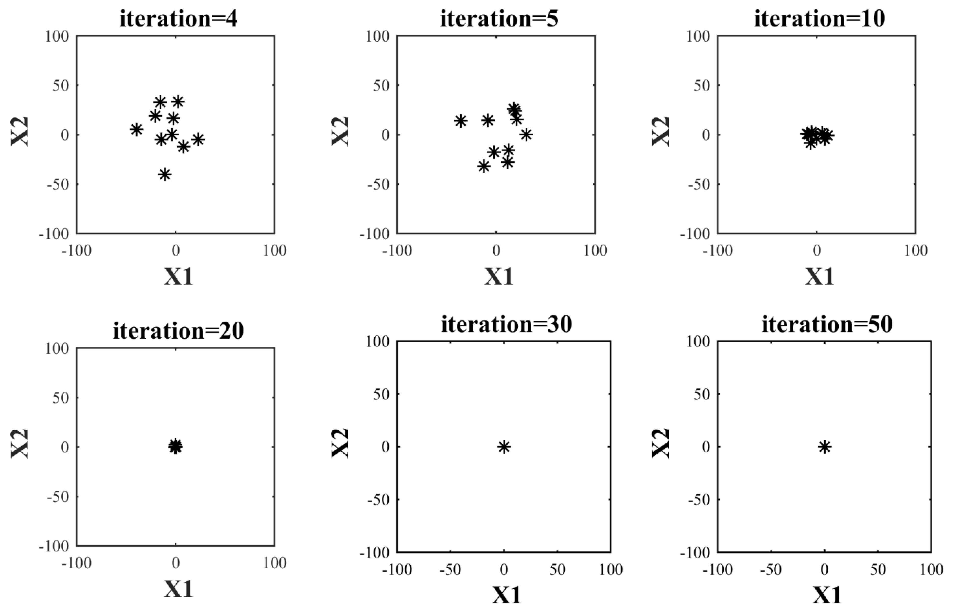
6. Exploration and Exploitation of the BSSA

The two most important indicators recommended for evaluating the performance of different optimization algorithms in optimizing optimization problems are exploitation power and exploration power. The exploitation index is used to analyze the ability of optimization algorithms to achieve the optimal solution. In fact, an algorithm that can provide a solution closer to the original solution has a higher power of exploitation. The exploration index is used for the analysis of the power of optimization algorithms in the exact search of the defined search space of a specific optimization problem. This indicator is especially important for optimization problems that have several local optimal points. Thus, an algorithm that can effectively scan the entire search space is able to extract the population of the algorithm from the local optimal points and direct it to the main optimal areas. Therefore, according to the definition of the mentioned indicators, it is better that the optimization algorithms have more exploratory power in the first iterations to examine different areas of the search space. Then, as the algorithm approaches the final iterations, the exploitation power of the algorithm must be adjusted to provide the appropriate solution [70,71].

The BSSA is able to accurately scan the search space according to the appropriate population members. The main parameter considered in the BSSA to maintain the balance between the two important indicators of exploitation and exploration is the spring constant. The equation of the spring constant in the BSSA is designed to have large values in the initial iterations and, as a result, according to Hooke’s law and spring force, different areas of the search space are scanned by members of the population. Then, by increasing the iterations of the algorithm and getting closer to the final iterations, the spring constant has smaller values and searches the optimal areas more carefully in order to provide the most appropriate solution possible. The above procedure is included in Equation (11) to adjust the spring constant and maintain the balance between the exploitation power and the exploration power.

7. Simulation Results

The performance of the BSSA was evaluated on 23 benchmark fitness test functions [72], as defined in

Table 2. Unimodal test functions.

$F_1\left(x\right)={{\displaystyle \sum }}_{i=1}^m{x}_i^2$	${\left[-100,100\right]}^m$
$F_2\left(x\right)={{\displaystyle \sum }}_{i=1}^m\left|x_i\right|+{{\displaystyle \prod }}_{i=1}^m\left|x_i\right|$	${\left[-10,10\right]}^m$
$F_3\left(x\right)={{\displaystyle \sum }}_{i=1}^m{\left({{\displaystyle \sum }}_{j=1}^i{x}_i\right)}^2$	${\left[-100,100\right]}^m$
$F_4\left(x\right)=max\left\{\left|x_i\right| , 1\le i\le m \right\}$	${\left[-100,100\right]}^m$
$F_5\left(x\right)={{\displaystyle \sum }}_{i=1}^{m-1}\left[100{\left(x_{i+1}-x_i^2\right)}^2+{\left(x_i-1\right)}^2)\right]$	${\left[-30,30\right]}^m$
$F_6\left(x\right)={{\displaystyle \sum }}_{i=1}^m{\left(\left[x_i+0.5\right]\right)}^2$	${\left[-100,100\right]}^m$
$F_7\left(x\right)={{\displaystyle \sum }}_{i=1}^{m}i{x}_i^4+random\left(0,1\right)$	${\left[-1.28,1.28\right]}^m$

,

Table 3. Multimodal test functions.

$F_8\left(x\right)={{\displaystyle \sum }}_{i=1}^m-x_i \sin \left(\sqrt{\left|x_i\right|}\right)$	${\left[-500,500\right]}^m$
$F_9\left(x\right)={{\displaystyle \sum }}_{i=1}^m\left[ x_i^2-10\cos \left(2\pi x_i\right)+10\right]$	${\left[-5.12,5.12\right]}^m$
$F_{10}\left(x\right)=-20\exp \left(-0.2\sqrt{\frac{1}{m}{{\displaystyle \sum }}_{i=1}^m{x}_i^2}\right)-\exp \left(\frac{1}{m}{{\displaystyle \sum }}_{i=1}^{m}cos\left(2\pi x_i\right)\right)+20+e$	${\left[-32,32\right]}^m$
$F_{11}\left(x\right)=\frac{1}{4000}{{\displaystyle \sum }}_{i=1}^m{x}_i^2-{{\displaystyle \prod }}_{i=1}^{m}cos\left(\frac{x_i}{\sqrt{i}}\right)+1$	${\left[-600,600\right]}^m$
$F_{12}\left(x\right)=\frac{\pi }{m} \left\{10\sin \left(\pi y_1\right)+{{\displaystyle \sum }}_{i=1}^m{\left(y_i-1\right)}^2\left[1+10{\sin }^2\left(\pi y_{i+1}\right)\right]+{\left(y_n-1\right)}^2\right\}+{{\displaystyle \sum }}_{i=1}^{m}u\left(x_i,10,100,4\right)$ $u\left(x_i,a,i,n\right)=\{\begin{array}{c}k{\left(x_i-a\right)}^n x_i>-a\\ 0 -a<x_i<a\\ k{\left(-x_i-a\right)}^n x_i<-a\end{array}$	${\left[-50,50\right]}^m$
$F_{13}\left(x\right)=0.1\left\{ {\sin }^2\left(3\pi x_1\right)+{{\displaystyle \sum }}_{i=1}^m{\left(x_i-1\right)}^2\left[1+{\sin }^2\left(3\pi x_i+1\right)\right]+{\left(x_n-1\right)}^2\left[1+{\sin }^2\left(2\pi x_m\right)\right]\right\}+{{\displaystyle \sum }}_{i=1}^{m}u\left(x_i,5,100,4\right)$	${\left[-50,50\right]}^m$

and

Table 4. Multimodal test functions with fixed dimensions.

$F_{14}\left(x\right)={\left(\frac{1}{500}+{{\displaystyle \sum }}_{j=1}^{25}\frac{1}{j+{{\displaystyle \sum }}_{i=1}^2{\left(x_i-a_{ij}\right)}^6}\right)}^{-1}$	${\left[-65.53,65.53\right]}^2$
$F_{15}\left(x\right)={{\displaystyle \sum }}_{i=1}^{11}{\left[a_i-\frac{x_1\left(b_i^2+b_i{x}_2\right)}{b_i^2+b_i{x}_3+x_4}\right]}^2$	${\left[-5,5\right]}^4$
$F_{16}\left(x\right)=4x_1^2-2.1x_1^4+\frac{1}{3}{x}_1^6+x_1{x}_2-4x_2^2+4x_2^4$	${\left[-5,5\right]}^2$
$F_{17}\left(x\right)={\left(x_2-\frac{5.1}{4{\pi }^2}{x}_1^2+\frac{5}{\pi }{x}_1-6\right)}^2+10\left(1-\frac{1}{8\pi }\right)cos{x}_1+10$	[–5,10] $\times$ [0,15]
$F_{18}\left(x\right)=\left[1+{\left(x_1+x_2+1\right)}^2\left(19-14x_1+3x_1^2-14x_2+6x_1{x}_2+3x_2^2\right)\right]\times \left[30+{\left(2x_1-3x_2\right)}^2\times \left(18-32x_1+12x_1^2+48x_2-36x_1{x}_2+27x_2^2\right)\right]$	${\left[-5,5\right]}^2$
$F_{19}\left(x\right)=-{{\displaystyle \sum }}_{i=1}^4{c}_i\exp \left(-{{\displaystyle \sum }}_{j=1}^3{a}_{ij}{\left(x_j-P_{ij}\right)}^2\right)$	${\left[0,1\right]}^3$
$F_{20}\left(x\right)=-{{\displaystyle \sum }}_{i=1}^4{c}_i\exp \left(-{{\displaystyle \sum }}_{j=1}^6{a}_{ij}{\left(x_j-P_{ij}\right)}^2\right)$	${\left[0,1\right]}^6$
$F_{21}\left(x\right)=-{{\displaystyle \sum }}_{i=1}^5{\left[\left(X-a_i\right){\left(X-a_i\right)}^T+6c_i\right]}^{-1}$	${\left[0,10\right]}^4$
$F_{22}\left(x\right)=-{{\displaystyle \sum }}_{i=1}^7{\left[\left(X-a_i\right){\left(X-a_i\right)}^T+6c_i\right]}^{-1}$	${\left[0,10\right]}^4$
$F_{23}\left(x\right)=-{{\displaystyle \sum }}_{i=1}^{10}{\left[\left(X-a_i\right){\left(X-a_i\right)}^T+6c_i\right]}^{-1}$	${\left[0,10\right]}^4$

.

The performance of the BSSA was compared with other algorithms, such as Binary Genetic Algorithm (BGA) [73], Binary Particle Swarm Optimization (BPSO) [65], Binary Gravitational Search Algorithm (BGSA) [74], Binary Bat Algorithm (BBA) [75], Binary Dragonfly Algorithm (BDA) [76], and Binary Grasshopper Optimization Algorithm (BGOA) [77].

Each optimization algorithm was applied independently 20 times, and the results were averaged. As can be seen from

Table 5. Results for the BSSA and other algorithms in unimodal test functions.

		BSSA	BGOA	BMOA	BBA	BDA	BGSA	BPSO	BGA
F1	Ave	6.74E−35	5.71E−28	4.61E−23	7.86E−10	2.81E−01	1.16E−16	4.98E−09	1.95E−12
	std	9.17E−36	8.31E−29	7.37E−23	8.11E−09	1.11E−01	6.10E−17	1.40E−08	2.01E−11
F2	Ave	7.78E−45	6.20E−40	1.20E−34	5.99E−20	3.96E−01	1.70E−01	7.29E−04	6.53E−18
	std	3.48E−45	3.32E−40	1.30E−34	1.11E−17	1.41E−01	9.29E−01	1.84E−03	5.10E−17
F3	Ave	2.63E−25	2.05E−19	1.00E−14	9.19E−05	4.31E+01	4.16E+02	1.40E+01	7.70E−10
	std	9.83E−27	9.17E−20	4.10E−14	6.16E−04	8.97E+00	1.56E+02	7.13E+00	7.36E−09
F4	Ave	4.65E−26	4.32E−18	2.02E−14	8.73E−01	8.80E−01	1.12E+00	6.00E−01	9.17E+01
	std	4.68E−29	3.98E−19	2.43E−14	1.19E−01	2.50E−01	9.89E−01	1.72E−01	5.67E+01
F5	Ave	5.41E−01	5.07E+00	2.79E+01	8.91E+02	1.18E+02	3.85E+01	4.93E+01	5.57E+02
	std	5.05E−02	4.90E−01	1.84E+00	2.97E+02	1.43E+02	3.47E+01	3.89E+01	4.16E+01
F6	Ave	8.03E−24	7.01E−19	6.58E−01	8.18E−17	3.15E−01	1.08E−16	9.23E−09	3.15E−01
	std	5.22E−26	4.39E−20	3.38E−01	1.70E−18	9.98E−02	4.00E−17	1.78E−08	9.98E−02
F7	Ave	3.33E−08	2.71E−05	7.80E−04	5.37E−01	2.02E−02	7.68E−01	6.92E−02	6.79E−04
	std	1.18E−06	9.26E−06	3.85E−04	1.89E−01	7.43E−03	2.77E+00	2.87E−02	3.29E−03

,

Table 6. Results for the BSSA and other algorithms in multimodal test functions.

		BSSA	BGOA	BMOA	BBA	BDA	BGSA	BPSO	BGA
F8	Ave	−1.2E+04	−8.76E+02	−6.14E+02	−4.69E+01	−6.92E+02	−2.75E+02	−5.01E+02	−5.11E+02
	std	9.14E−12	5.92E+01	9.32E+01	3.94E+01	9.19EE+01	5.72E+01	4.28E+01	4.37E+01
F9	Ave	8.76E−04	6.90E−01	4.34E−01	4.85E−02	1.01E+02	3.35E+01	1.20E−01	1.23E−01
	std	4.85E−02	4.81E−01	1.66E+00	3.91E+01	1.89E+01	1.19E+01	4.01E+01	4.11E+01
F10	Ave	8.04E−20	8.03E−16	1.63E−14	2.83E−08	1.15E+00	8.25E−09	5.20E−11	5.31E−11
	std	3.34E−18	2.74E−14	3.14E−15	4.34E−07	7.87E−01	1.90E−09	1.08E−10	1.11E−10
F11	Ave	4.23E−10	4.20E−05	2.29E−03	2.49E−05	5.74E−01	8.19E+00	3.24E−06	3.31E−06
	std	5.11E−07	4.73E−04	5.24E−03	1.34E−04	1.12E−01	3.70E+00	4.11E−05	4.23E−05
F12	Ave	6.33E−08	5.09E−03	3.93E−02	1.34E−05	1.27E+00	2.65E−01	8.93E−08	9.16E−08
	std	4.71E−04	3.75E−03	2.42E−02	6.23E−04	1.02E+00	3.14E−01	4.77E−07	4.88E−07
F13	Ave	0.00E+00	1.25E−08	4.75E−01	9.94E−08	6.60E−02	5.73E−32	6.26E−02	6.39E−02
	std	0.00E+00	2.61E−07	2.38E−01	2.61E−07	4.33E−02	8.95E−32	4.39E−02	4.49E−02

and

Table 7. Results for the BSSA and other algorithms in multimodal test functions with fixed dimensions.

		BSSA	BGOA	BMOA	BBA	BDA	BGSA	BPSO	BGA
F14	Ave	9.98E−01	1.08E+00	3.71E+00	1.26E+00	9.98E+01	3.61E+00	2.77E+00	4.39E+00
	std	7.64E−12	4.11E−02	3.86E+00	6.86E−01	9.14E−1	2.96E+00	2.32E+00	4.41E−02
F15	Ave	3.3E−04	8.21E−03	3.66E−02	1.01E−02	7.15E−02	6.84E−02	9.09E−03	7.36E−02
	std	1.25E−05	4.09E−03	7.60E−02	3.75E−03	1.26E−01	7.37E−02	2.38E−03	2.39E−03
F16	Ave	−1.03E+00	−1.02E+00	−1.02E+00	−1.02E+00	−1.02E+00	−1.02E+00	−1.02E+00	−1.02E+00
	std	5.12E−10	9.80E−07	7.02E−09	3.23E−05	4.74E−08	0.00E+00	0.00E+00	4.19E−07
F17	Ave	3.98E−01	3.98E−01	3.98E−01	3.98E−01	3.98E−01	3.98E−01	3.98E−01	3.98E−01
	std	4.56E−21	5.39E−05	7.00E−07	7.61E−04	1.15E−07	1.13E−16	9.03E−16	3.71E−17
F18	Ave	3.00E+00	3.00E+00	3.00E+00	3.00E+00	3.00E+00	3.00E+00	3.00E+00	3.00E+00
	std	1.15E−18	1.15E−08	7.16E−06	2.25E−05	1.48E+01	3.24E−02	6.59E−05	6.33E−07
F19	Ave	−3.86E+00	−3.86E+00	−3.84E+00	−3.75E+00	−3.77E+00	−3.86E+00	−3.80E+00	−3.81E+00
	std	5.61E−10	6.50E−07	1.57E−03	2.55E−03	3.53E−07	4.15E−01	3.37E−15	4.37E−10
F20	Ave	−3.32E+00	−2.81E+00	−3.27E+00	−2.84E+00	−3.23E+00	−1.47E+00	−3.32E+00	−2.39E+00
	std	4.29E−05	7.11E−01	7.27E−02	3.71E−01	5.37E−02	5.32E−01	2.66E−01	4.37E−01
F21	Ave	−10.15E+00	−8.07E+00	−9.65E+00	−2.28E+00	−7.38E+00	−4.57E+00	−7.54E+00	−5.19E+00
	std	1.25E−02	2.29E+00	1.54E+00	1.80E+00	2.91E+00	1.30E+00	2.77E+00	2.34E+00
F22	Ave	−10.40E+00	−10.01E+00	−1.04E+00	−3.99E+00	−8.50E+00	−6.58E+00	−8.55E+00	−2.97E+00
	std	3.65E−07	3.97E−02	2.73E−04	1.99E+00	3.02E+00	2.64E+00	3.08E+00	1.37E−02
F23	Ave	−10.53E+00	−3.41E+00	−1.05E+01	−4.49E+00	−8.41E+00	−9.37E+00	−9.19E+00	−3.10E+00
	std	5.26E−06	1.11E−02	1.81E−04	1.96E+00	3.13E+00	2.75E+00	2.52E+00	2.37E+00

, the BSSA provides better results for most functions.

The seven objective functions F1–F7 are suitable for evaluating the exploitation rate. Based on the optimization results presented, Table 5 shows that the proposed algorithm is the best. The objective functions F8–F23 were selected to study and analyze the scan index. The optimization of the objective functions in Table 6 and Table 7 shows the exploitability of the algorithm.

Statistical Testing

Although the simulation and optimization results, reported as the average of the best solution and standard deviation, indicate the superiority of the proposed BSSA, these results alone are not sufficient to guarantee the proposed algorithm’s superiority. Although all algorithms were run independently 20 times, it is still possible that the advantage occurs by chance despite its low probability in 20 runs. Therefore, the Friedman rank test [78] was applied to analyze the results further. This statistical test has two approaches to achieving the same goal. A quantitative variable is recorded two or more times in the same sample. In the other objective, the quantitative variables are measured from the same sample. In these objectives, the Friedman test compares the distributions (of the two or more quantitative variables). The results of this test are presented in

Table 8. Results of the Friedman rank test.

Test Function			BGA	BPSO	BGSA	BDA	BBA	BMOA	BGOA	BSSA
1	Unimodal (F1–F7)	Friedman value	39	39	42	46	38	26	14	7
		Friedman rank	5	5	6	7	4	3	2	1
2	Multimodal (F8–F13)	Friedman value	25	21	36	40	28	31	22	6
		Friedman rank	4	2	7	8	5	6	3	1
3	Multimodal with fixed dimensions (F14–F23)	Friedman value	52	31	42	44	44	34	29	10
		Friedman rank	7	3	5	6	6	4	2	1
4	All 23 test functions	Friedman value	116	91	120	130	110	91	65	23
		Friedman rank	5	3	6	7	4	3	2	1

and are specified for all three different groups of objective functions: unimodal, multimodal, and multimodal with fixed dimension test functions and all objective test functions. Based on these results, the proposed algorithm for all three different test functions is positioned first in the Friedman rank test. Furthermore, the overall results of all the test functions (F₁–F₂₃) show that the BSSA is significantly superior to the other algorithms.

8. Conclusions

There are many optimization problems that must be solved by using a suitable method. Different heuristic optimization algorithms have been proposed to overcome the shortcomings of traditional methods, such as Linear Programming (LP), non-linear LP, and differential programming. Most of these algorithms are population-based using the randomness of natural phenomena. A heuristic optimization algorithm called Binary Spring Search Algorithm (BSSA) is proposed, which uses laws of the spring force law. The proposal was mathematically modeled, and its efficiency was evaluated using 23 standard test functions. These test functions were selected from three different types: unimodal, multimodal, and multimodal with fixed dimension test functions to evaluate different aspects of the proposed algorithm. Seven optimization algorithms (binary genetic algorithm, binary particle swarm optimization, binary gravitational search algorithm, binary dragonfly algorithm, binary bat algorithm, and binary grasshopper optimization algorithm) were compared to evaluate the performance of the proposed algorithm. Compared to the other algorithms, in all cases, the BSSA produces nearly optimal solutions. Friedman’s rank test was used to further analyze the performance of the BSSA. The results obtained from this test show the clear superiority of the proposed algorithm in the three different types of test functions. The overall results of all test functions (F1–F23) show that the BSSA is significantly superior to the other algorithms and ranks first among them. Based on the optimization results and the Friedman rank test results, it is clear that the proposed BSSA performs well in solving optimization problems and is more competitive than similar algorithms.

References

1. Dehghani, M.; Samet, H. Momentum search algorithm: A new meta-heuristic optimization algorithm inspired by momentum conservation law. SN Appl. Sci. 2020, 2, 1720. [Google Scholar] [CrossRef]
2. Dehghani, M.; Montazeri, Z.; Dehghani, A.; Samet, H.; Sotelo, C.; Sotelo, D.; Ehsanifar, A.; Malik, O.P.; Guerrero, J.M.; Dhiman, G.; et al. DM: Dehghani Method for Modifying Optimization Algorithms. Appl. Sci. 2020, 10, 7683. [Google Scholar] [CrossRef]
3. Dehghani, M.; Montazeri, Z.; Dhiman, G.; Malik, O.P.; Morales-Menendez, R.; Ramirez-Mendoza, R.A.; Dehghani, A.; Guerrero, J.M.; Parra-Arroyo, L. A Spring Search Algorithm Applied to Engineering Optimization Problems. Appl. Sci. 2020, 10, 6173. [Google Scholar] [CrossRef]
4. Dehghani, M.; Montazeri, Z.; Malik, O. Energy Commitment: A Planning of Energy Carrier Based on Energy Consumption. Electr. Eng. Electromech. 2019, 4, 69–72. [Google Scholar] [CrossRef]
5. Dehghani, M.; Mardaneh, M.; Malik, O.P.; Guerrero, J.M.; Sotelo, C.; Sotelo, D.; Nazari-Heris, M.; Al-Haddad, K.; Ramirez-Mendoza, R.A. Genetic Algorithm for Energy Commitment in a Power System Supplied by Multiple Energy Carriers. Sustainability 2020, 12, 10053. [Google Scholar] [CrossRef]
6. Ehsanifar, A.; Dehghani, M.; Allahbakhshi, M. Calculating the leakage inductance for transformer inter-turn fault detection using finite element method. In Proceedings of the 2017 Iranian Conference on Electrical Engineering (ICEE), Tehran, Iran, 2–4 May 2017; pp. 1372–1377. [Google Scholar]
7. Dehghani, M.; Montazeri, Z.; Malik, O.P. Optimal Sizing and Placement of Capacitor Banks and Distributed Generation in Distribution Systems Using Spring Search Algorithm. Int. J. Emerg. Electr. Power Syst. 2020, 21. [Google Scholar] [CrossRef] [Green Version]
8. Dehghani, M.; Montazeri, Z.; Malik, O.P.; Al-Haddad, K.; Guerrero, J.M.; Dhiman, G. A New Methodology Called Dice Game Optimizer for Capacitor Placement in Distribution Systems. Electr. Eng. Electromech. 2020, 1, 61–64. [Google Scholar] [CrossRef] [Green Version]
9. Dehbozorgi, S.; Ehsanifar, A.; Montazeri, Z.; Dehghani, M.; Seifi, A. Line loss reduction and voltage profile improvement in radial distribution networks using battery energy storage system. In Proceedings of the 2017 IEEE 4th International Conference on Knowledge-Based Engineering and Innovation (KBEI), Tehran, Iran, 22–22 December 2017; pp. 0215–0219. [Google Scholar]
10. Montazeri, Z.; Niknam, T. Optimal Utilization of Electrical Energy from Power Plants Based on Final Energy Consumption Using Gravitational Search Algorithm. Electr. Eng. Electromech. 2018, 4, 70–73. [Google Scholar] [CrossRef] [Green Version]
11. Dehghani, M.; Mardaneh, M.; Montazeri, Z.; Ehsanifar, A.; Ebadi, M.J.; Grechko, O. Spring Search Algorithm for Simultaneous Placement of Distributed Generation and Capacitors. Electr. Eng. Electromech. 2018, 6, 68–73. [Google Scholar] [CrossRef]
12. Pelusi, D.; Mascella, R.; Tallini, L.G. A Fuzzy Gravitational Search Algorithm to Design Optimal IIR Filters. Energies 2018, 11, 736. [Google Scholar] [CrossRef] [Green Version]
13. Dehghani, M.; Montazeri, Z.; Ehsanifar, A.; Seifi, A.; Ebadi, M.; Grechko, O.M. Planning of Energy Carriers Based on Final Energy Consumption Using Dynamic Programming and Particle Swarm Optimization. Electr. Eng. Electromech. 2018, 5, 62–71. [Google Scholar] [CrossRef] [Green Version]
14. Montazeri, Z.; Niknam, T. Energy carriers management based on energy consumption. In Proceedings of the 2017 IEEE 4th International Conference on Knowledge-Based Engineering and Innovation (KBEI), Tehran, Iran, 22–22 December 2017; pp. 0539–0543. [Google Scholar]
15. Pelusi, D.; Mascella, R.; Tallini, L.G.; Nayak, J.; Naik, B.; Deng, Y. Improving exploration and exploitation via a Hyperbolic Gravitational Search Algorithm. Knowl. Based Syst. 2020, 193, 105404. [Google Scholar] [CrossRef]
16. Pelusi, D.; Mascella, R.; Tallini, L.G.; Nayak, J.; Naik, B.; Deng, Y. An Improved Moth-Flame Optimization algorithm with hybrid search phase. Knowl. Based Syst. 2020, 191, 105277. [Google Scholar] [CrossRef]
17. Pelusi, D.; Mascella, R.; Tallini, L.G.; Nayak, J.; Naik, B.; Abraham, A. Neural network and fuzzy system for the tuning of Gravitational Search Algorithm parameters. Expert Syst. Appl. 2018, 102, 234–244. [Google Scholar] [CrossRef]
18. Gigerenzer, G.; Todd, P.M. Simple Heuristics that Make Us Smart; Oxford University Press: New York, NY, USA, 1999. [Google Scholar]
19. Lazar, A. Heuristic knowledge discovery for archaeological data using genetic algorithms and rough sets. Heuristics Optim. Knowl. Discov. 2002, 263. [Google Scholar] [CrossRef]
20. Gigerenzer, G.; Gaissmaier, W. Heuristic Decision Making. Annu. Rev. Psychol. 2011, 62, 451–482. [Google Scholar] [CrossRef] [Green Version]
21. Kirkpatrick, S.; Gelatt, C.D.; Vecchi, M.P. A heuristic algorithm and simulation approach to relative location of facilities. Optim. Simulated Annealing 1983, 220, 671–680. [Google Scholar]
22. Shah-Hosseini, H. Principal components analysis by the galaxy-based search algorithm: A novel metaheuristic for continuous optimisation. Int. J. Comput. Sci. Eng. 2011, 6, 132. [Google Scholar] [CrossRef]
23. Kaveh, A.; Talatahari, S. A novel heuristic optimization method: Charged system search. Acta Mech. 2010, 213, 267–289. [Google Scholar] [CrossRef]
24. Moghaddam, F.F.; Moghaddam, R.F.; Cheriet, M. Curved space optimization: A random search based on general relativity theory. arXiv 2012, arXiv:1208.2214. [Google Scholar]
25. Alatas, B. ACROA: Artificial Chemical Reaction Optimization Algorithm for global optimization. Expert Syst. Appl. 2011, 38, 13170–13180. [Google Scholar] [CrossRef]
26. Kaveh, A.; Khayatazad, M. A new meta-heuristic method: Ray Optimization. Comput. Struct. 2012, 112, 283–294. [Google Scholar] [CrossRef]
27. Du, H.; Wu, X.; Zhuang, J. Small-World Optimization Algorithm for Function Optimization. In Proceedings of the Second International Conference on Advances in Natural Computation; Springer: Berlin/Heidelberg, Germany, 2006; pp. 264–273. [Google Scholar]
28. Hatamlou, A. Black hole: A new heuristic optimization approach for data clustering. Inf. Sci. 2013, 222, 175–184. [Google Scholar] [CrossRef]
29. Formato, R.A. Central force optimization: A new nature inspired computational framework for multidimensional search and optimization. In Nature Inspired Cooperative Strategies for Optimization (NICSO 2007); Springer: Berlin/Heidelberg, Germany, 2008; pp. 221–238. [Google Scholar]
30. Erol, O.K.; Eksin, I. A new optimization method: Big Bang–Big Crunch. Adv. Eng. Softw. 2006, 37, 106–111. [Google Scholar] [CrossRef]
31. Kennedy, J.; Eberhart, R. Particle swarm optimization. In Proceedings of the IEEE International Conference on Neural Networks, Perth, Australia, 27 November–1 December 1995; IEEE Service Center: Piscataway, NY, USA, 1942; Volume 1948. [Google Scholar]
32. Yang, X.-S. A new metaheuristic bat-inspired algorithm. In Nature Inspired Cooperative Strategies for Optimization (NICSO 2010); Springer: Berlin/Heidelberg, Germany, 2010; pp. 65–74. [Google Scholar]
33. Karaboga, D.; Basturk, B. Artificial bee colony (ABC) optimization algorithm for solving constrained optimization, problems. In Proceedings of the 12th International Fuzzy Systems Association World Congress on Foundations of Fuzzy Logic and Soft Computing; Springer: Berlin/Heidelberg, Germany, 2007. [Google Scholar]
34. Dehghani, M.; Mardaneh, M.; Guerrero, J.M.; Malik, O.P.; Ramirez-Mendoza, R.A.; Matas, J.; Vasquez, J.C.; Parra-Arroyo, L. A New “Doctor and Patient” Optimization Algorithm: An Application to Energy Commitment Problem. Appl. Sci. 2020, 10, 5791. [Google Scholar] [CrossRef]
35. Gandomi, A.H.; Yang, X.-S.; Alavi, A.H. Cuckoo search algorithm: A metaheuristic approach to solve structural optimization problems. Eng. Comput. 2013, 29, 17–35. [Google Scholar] [CrossRef]
36. Dhiman, G.; Kumar, V. Spotted hyena optimizer: A novel bio-inspired based metaheuristic technique for engineering applications. Adv. Eng. Softw. 2017, 114, 48–70. [Google Scholar] [CrossRef]
37. Dehghani, M.; Montazeri, Z.; Dehghani, A.; Mendoza, R.R.; Samet, H.; Guerrero, J.M.; Dhiman, G. MLO: Multi Leader Optimizer. Int. J. Intell. Eng. Syst. 2020, 13, 364–373. [Google Scholar] [CrossRef]
38. Dehghani, M.; Montazeri, Z.; Dehghani, A.; Malik, O.P. GO: Group Optimization. GAZI Univ. J. Sci. 2020, 33, 381–392. [Google Scholar] [CrossRef]
39. Mucherino, A.; Seref, O. Monkey Search: A Novel Metaheuristic Search for Global Optimization. AIP Conf. Proc. 2007, 953, 162–173. [Google Scholar]
40. Mirjalili, S.; Mirjalili, S.M.; Lewis, A. Grey wolf optimizer. Adv. Eng. Softw. 2014, 69, 46–61. [Google Scholar] [CrossRef] [Green Version]
41. Neshat, M.; Sepidnam, G.; Sargolzaei, M.; Toosi, A.N. Artificial fish swarm algorithm: A survey of the state-of-the-art, hybridization, combinatorial and indicative applications. Artif. Intell. Rev. 2014, 42, 965–997. [Google Scholar] [CrossRef]
42. Oftadeh, R.; Mahjoob, M.J.; Shariatpanahi, M. A novel meta-heuristic optimization algorithm inspired by group hunting of animals: Hunting search. Comput. Math. Appl. 2010, 60, 2087–2098. [Google Scholar] [CrossRef] [Green Version]
43. Mirjalili, S. Moth-flame optimization algorithm: A novel nature-inspired heuristic paradigm. Knowl. Based Syst. 2015, 89, 228–249. [Google Scholar] [CrossRef]
44. Dhiman, G.; Kumar, V. Emperor penguin optimizer: A bio-inspired algorithm for engineering problems. Knowl. Based Syst. 2018, 159, 20–50. [Google Scholar] [CrossRef]
45. Shiqin, Y.; Jianjun, J.; Guangxing, Y. A dolphin partner optimization. In Proceedings of the Global Congress on Intelligent Systems, Xiamen, China, 19–21 May 2009; pp. 124–128. [Google Scholar]
46. Dehghani, M.; Mardaneh, M.; Malik, O.P.; NouraeiPour, S.M. DTO: Donkey Theorem Optimization. In Proceedings of the 2019 27th Iranian Conference on Electrical Engineering (ICEE), Yazd, Iran, 30 April–2 May 2019; pp. 1855–1859. [Google Scholar]
47. Dhiman, G.; Garg, M.; Nagar, A.; Kumar, V.; Dehghani, M. A novel algorithm for global optimization: Rat Swarm Optimizer. J. Ambient. Intell. Humaniz. Comput. 2020. [Google Scholar] [CrossRef]
48. Saremi, S.; Mirjalili, S.; Lewis, A. Grasshopper Optimisation Algorithm: Theory and application. Adv. Eng. Softw. 2017, 105, 30–47. [Google Scholar] [CrossRef]
49. Zhang, H.; Hui, Q. A Coupled Spring Forced Bat Searching Algorithm: Design, Analysis and Evaluation. In Proceedings of the 2020 American Control Conference (ACC), Denver, CO, USA, 1–3 July 2020; pp. 5016–5021. [Google Scholar]
50. Dehghani, M.; Mardaneh, M.; Malik, O. FOA: ‘Following’ Optimization Algorithm for solving power engineering optimization problems. J. Oper. Autom. Power Eng. 2020, 8, 57–64. [Google Scholar]
51. Dehghani, M.; Mardaneh, M.; Guerrero, J.M.; Malik, O.P.; Kumar, V. Football Game Based Optimization: An Application to Solve Energy Commitment Problem. Int. J. Intell. Eng. Syst. 2020, 13, 514–523. [Google Scholar] [CrossRef]
52. Dehghani, M.; Montazeri, Z.; Malik, O.P.; Dhiman, G.; Kumar, V. BOSA: Binary Orientation Search Algorithm. Int. J. Innov. Technol. Explor. Eng. 2019, 9, 5306–5310. [Google Scholar]
53. Dehghani, M.; Montazeri, Z.; Givi, H.; Guerrero, J.M.; Dhiman, G. Darts Game Optimizer: A New Optimization Technique Based on Darts Game. Int. J. Intell. Eng. Syst. 2020, 13, 286–294. [Google Scholar] [CrossRef]
54. Dehghani, M.; Montazeri, Z.; Malik, O.P.; Ehsanifar, A.; Dehghani, A. OSA: Orientation Search Algorithm. Int. J. Ind. Electron. Control Optim. 2019, 2, 99–112. [Google Scholar]
55. Mohammad, D.; Zeinab, M.; Malik, O.P.; Givi, H.; Guerrero, J.M. Shell Game Optimization: A Novel Game-Based Algorithm. Int. J. Intell. Eng. Syst. 2020, 13, 246–255. [Google Scholar] [CrossRef]
56. Dehghani, M.; Montazeri, Z.; Malik, O.P. DGO: Dice Game Optimizer. GAZI Univ. J. Sci. 2019, 32, 871–882. [Google Scholar] [CrossRef] [Green Version]
57. Dehghani, M.; Montazeri, Z.; Saremi, S.; Dehghani, A.; Malik, O.P.; Al-Haddad, K.; Guerrero, J.M. HOGO: Hide Objects Game Optimization. Int. J. Intell. Eng. Syst. 2020, 13, 216–225. [Google Scholar] [CrossRef]
58. Holland, J.H. Genetic algorithms. Sci. Am. 1992, 267, 66–73. [Google Scholar] [CrossRef]
59. Deng, W.; Liu, H.; Xu, J.; Zhao, H.; Song, Y. An Improved Quantum-Inspired Differential Evolution Algorithm for Deep Belief Network. IEEE Trans. Instrum. Meas. 2020, 69, 7319–7327. [Google Scholar] [CrossRef]
60. Das, S.; Suganthan, P.N. Differential Evolution: A Survey of the State-of-the-Art. IEEE Trans. Evol. Comput. 2011, 15, 4–31. [Google Scholar] [CrossRef]
61. Simon, D. Biogeography-Based Optimization. IEEE Trans. Evol. Comput. 2008, 12, 702–713. [Google Scholar] [CrossRef] [Green Version]
62. Fogel, L.J.; Owens, A.J.; Walsh, M.J. Artificial Intelligence through Simulated Evolution; Wiley: NewYork, NY, USA, 1966. [Google Scholar]
63. Beyer, H.-G.; Schwefel, H.-P. Evolution strategies—A comprehensive introduction. Nat. Comput. 2002, 1, 3–52. [Google Scholar] [CrossRef]
64. Koza, J.R. Genetic programming as a means for programming computers by natural selection. Stat. Comput. 1994, 4, 87–112. [Google Scholar] [CrossRef]
65. Mirjalili, S. Particle Swarm Optimisation. In Evolutionary Algorithms and Neural Networks; Springer: Berlin/Heidelberg, Germany, 2019; pp. 15–31. [Google Scholar]
66. Tarasewich, P.; McMullen, P.R. Swarm intelligence: Power in numbers. Commun. ACM 2002, 45, 62–67. [Google Scholar] [CrossRef]
67. Kohonen, T. Self-Organization and Associative Memory; Springer Science & Business Media: Berlin/Heidelberg, Germany, 2012; Volume 8. [Google Scholar]
68. Dehghani, M.; Montazeri, Z.; Dehghani, A.; Nouri, N.; Seifi, A. BSSA: Binary spring search algorithm. In Proceedings of the 2017 IEEE 4th International Conference on Knowledge-Based Engineering and Innovation (KBEI), Tehran, Iran, 22–22 December 2017; pp. 220–224. [Google Scholar]
69. Halliday, D.; Resnick, R.; Walker, J. Fundamentals of Physics; John Wiley & Sons: Hoboken, NJ, USA, 2013. [Google Scholar]
70. Eiben, A.E.; Schippers, C.A. On Evolutionary Exploration and Exploitation. Fundam. Inform. 1998, 35, 35–50. [Google Scholar] [CrossRef]
71. Lynn, N.; Suganthan, P.N. Heterogeneous comprehensive learning particle swarm optimization with enhanced exploration and exploitation. Swarm Evol. Comput. 2015, 24, 11–24. [Google Scholar] [CrossRef]
72. Zhang, L.; Tang, Y.; Hua, C.; Guan, X. A new particle swarm optimization algorithm with adaptive inertia weight based on Bayesian techniques. Appl. Soft Comput. 2015, 28, 138–149. [Google Scholar] [CrossRef]
73. Castillo, O.; Aguilar, L.T. Genetic Algorithms. In Type-2 Fuzzy Logic in Control of Nonsmooth Systems; Springer: Berlin/Heidelberg, Germany, 2019; pp. 23–39. [Google Scholar]
74. Bala, I.; Yadav, A. Gravitational Search Algorithm: A State-of-the-Art Review. In Harmony Search and Nature Inspired Optimization Algorithms; Springer: Berlin/Heidelberg, Germany, 2019; pp. 27–37. [Google Scholar]
75. Mirjalili, S.; Mirjalili, S.M.; Yang, X.-S. Binary bat algorithm. Neural Comput. Appl. 2014, 25, 663–681. [Google Scholar] [CrossRef]
76. Mafarja, M.M.; Eleyan, D.; Jaber, I.; Hammouri, A.; Mirjalili, S. Binary Dragonfly Algorithm for Feature Selection. In Proceedings of the 2017 International Conference on New Trends in Computing Sciences (ICTCS), Amman, Jordan, 11–13 October 2017; pp. 12–17. [Google Scholar]
77. Mafarja, M.; Aljarah, I.; Faris, H.; Hammouri, A.I.; Ala’M, A.-Z.; Mirjalili, S. Binary grasshopper optimisation algorithm approaches for feature selection problems. Expert Syst. Appl. 2019, 117, 267–286. [Google Scholar] [CrossRef]
78. Daniel, W.W. Friedman two-way analysis of variance by ranks. In Applied Nonparametric Statistics; PWS-Kent: Boston, MA, USA, 1990; pp. 262–274. [Google Scholar]
Figure 1. The flowchart of the Binary Spring Search Algorithm (BSSA).
Applsci 11 01286 g001
Figure 2. Search space for the test function in the BSSA.
Applsci 11 01286 g002aApplsci 11 01286 g002b
Figure 3. Each object is displaced according to spring forces applied to it in the BSSA.
Applsci 11 01286 g003