1. Introduction and Motivations
The present work is placed in the context of the design of reliable algorithms for solving Data Assimilation (DA) for dynamic systems applications. DA is an uncertainty quantification technique by which measurements and model predictions are combined in order to obtain an accurate estimation of the state of the modelled system [
1]. In the past 20 years, DA methodologies, used, in principle, mainly in atmospheric models, has become a main component in the development and validation of mathematical models in meteorology, climatology, geophysics, geology, and hydrology (often these models are referred to with the term predictive to underline that these are dynamical systems). Recently, DA has also been applied to numerical simulations of geophysical applications [
2], medicine, and biological science [
3,
4] for improving the reliability of the numerical simulations. In practice, DA provides the answers to questions, such as: how well does the model under consideration represent the physical phenomena? What confidence can one have that the numerical results produced by the model are correct? How far can the calculated results be extrapolated? How can the predictability and/or extrapolation limits be extended and/or improved?
Accuracy in numerical models of dynamic systems does not come easily. The simulation errors come from three main sources: inaccurate input data, inaccurate physics models, and limited accuracy of the numerical solutions of the governing equations. Our ability to predict any physical phenomenon is determined by the accuracy of our input data and our modelling approach [
5]. Errors arise at the different stages of the solution process, namely, the uncertainty in the mathematical model, in the model’s solution, and in the measurements. These are the errors intrinsic to the DA problem. Moreover, there are the approximation errors that are introduced by the linearization, the discretization, and the model reduction. These errors incur when infinite-dimensional equations are replaced by a finite-dimensional system (that is, the process of discretization), or when simpler approximations to the equations are developed (e.g., by model reduction). Finally, given the numerical problem, an algorithm is developed and implemented as a mathematical software. At this stage, the inevitable rounding errors introduced by working in finite-precision arithmetic occur. These approaches are unable to fully overcome their unrealistic assumptions, particularly linearity, normality, and zero error covariances, despite the improvements in the complexity of the DA models to better match their application requirements and circumvent their implementation problems [
6].
With the rapid developments in recent years, DL shows great capability in approximating nonlinear systems, and extracting high dimensional features. As the foundation and main driving force of deep learning, DNN is concerned less about numerical modelling. DNN took a data driven approach, where the models are built by learning from data. Instead of being deterministic [
7,
8], DL models such as NN are stochastic. Thus, they can well succeed when applied to deterministic systems, but without ever learning the relationship between the variables. For e.g., ML algorithms do not know when they violate the physics laws of [
9,
10] in weather forecasting. Before they begin to produce accurate results, machine learning methods often need large quantities of data, and, the bigger the architecture, the more data are required. In a wide variety of applications, DL is successfully used when the conditions allow. However, in cases where the dimensions are either very large, the data are noisy or the data do not cover the entire domain adequately; these approaches still fail. Furthermore, the network will not perform well if the available information is too noisy, too scarce, or if there is a lack of prominent features to reflect the problem. This can occur either if there is a lack of good characteristics or a lack of data on good ground reality. For this reason, a good quality of the data (smaller errors) can help to generate a more reliable DNN. DA is the Bayesian approximation of the true state of some physical system at a given time by combining time-distributed observations with a dynamic model in an optimal way. In some sense, DA increases the meaningfulness of the data and reduces the forecasting errors. Therefore, it is interesting to investigate the mechanism where two data driven paradigms, DA and DNN, can be integrated.
In this context, we developed the Deep Data Assimilation (DDA) model. DDA is a new concept that combines the DNN and DA. It faces the problem to reduce both input data error (by DA) and modelling error (by ML).
Related Works and Contribution of the Present Work
This paper is placed in the imperfect models and sensitivity analysis context for data assimilation and deep neural network. Sensitivity Analysis (SA) refers to the determination of the contributions of individual uncertainty on data to the uncertainty in the solution [
11]. The sensitivity of the variational DA models has been studied in [
12], where an Adjoint modeling is used in order to obtain first and second-order derivative information. In [
13], sensitivity analysis is based on the Backward Error Analysis (B.E.A.), which figure out how much the errors propagation in DA process depend on the condition number of the background error covariance matrices. Reduced-order approaches are formulated in [
12] in order to alleviate the computational cost that is associated with the sensitivity estimation. This method makes rerunning less expensive, the parameters must still be selected a priori and, consequently, important sensitivities may be missed [
14]. For imperfect models, weak constraint DA (WCDA) can be employed [
15], in which the model error term in the covariance evolution equation acts to reduce the dependence of the estimate on observations and prior states that are well separated in time. However, the time complexity of the WCDA models is a big limit that makes these models often unusable.
ML algorithms are capable of assisting or replacing, without the assumptions of traditional methods, the aforementioned conventional methods in assimilating data, and producing forecasts. Because any linear or nonlinear functions can be approximated by neural networks, DA has been integrated as a supplement in various applications. The technology and the model presented in this paper are very general and they can be applied to any kind of dynamical systems. The use of ML in correcting model forecasts is promising in several geophysics applications [
16,
17]. Babovic [
18,
19,
20] applies neural network for error correction in forecasting. However, in this literature, the error correction neural network has not a direct relation with the system update model in each step and it does not train the results of the assimilation process. In [
21], DA and ML are also integrated and a surrogate model is used in order to replace the dynamical system. In this paper we do not replace the the dynamical system with a surrogate models, as this would add approximation errors. In fact, in real case scenarios (i.e., in some operational centres), data driven models are welcome to support Computational Fluid Dynamics simulations [
9,
10,
22], but the systems of Partial Differential Equations that are stably implemented to predict (weather, climate, ocean, air pollution, et al.) dynamics are not replaced due to the big approximations that this replacement would introduce. The technology that we propose in this paper integrates DA with ML in a way that can be used in real case scenarios for real world applications without changing the already implemented dynamical systems.
Other works have already explored the relationship between the learning, analysis, and implementation of data in ML and DA. These studies have concentrated on fusing methods from the two fields instead of taking a modular approach like the one implemented in this paper, thereby developing methods that are unique to those approaches. The integration of the DA and ML frameworks from a Bayesian perspective illustrates the interface between probabilistic ML methods and differential equations. The equivalence is formally presented in [
23] and it illustrates the parallels between the two fields. Here, the equivalence of four-dimensional VarDA (4D-Var) and Recurrent NN, and how approximate Bayesian inverse methods (i.e., VarDA in DA and back-propagation in ML) can be used to merge the two fields. These methods are also especially suited to systems involving Gaussian process, as presented in [
24,
25,
26]. These are developed data-driven algorithms that are capable, under a unified approach, of learning nonlinear, space-dependent cross-correlations, and of estimating model statistics. A DA method can be used via the DL framework to help the dynamic model (in this case, the ML model) to find optimal initial conditions. Although DA can be computationally costly, the recent dimensional reduction developments using ML substantially reduce this expense, while retaining much of the variance of the original [
27] model. Therefore, DA helps to develop the ML model, while [
28,
29] also benefits from the ML techniques. Methods that merge DA models, such as Kalman filters and ML, exist to overcome noise or to integrate time series knowledge. The authors account for temporal details in human motion analysis in [
30] by incorporating a Kalman filter into a neural network of LSTM. In [
31], the authors suggest a methodology that combines NN and DA for model error correction. Instead, in [
32], the authors use DA, in particular Kalman tracking, to speed up any learning-based motion tracking method to real-time and to correct some common inconsistencies in motion tracking methods that are based on the camera. Finally, in [
33], the authors introduce a new neural network for speed and replace the whole DA process.
In this paper, we proposed a new concept, called DDA, which combines the DL into the conventional DA. In recent years, DL gained great success both in academic and industrial areas. In function approximation, which has unknown model and high nonlinearity, it shows great benefit. Here, we use DNN to describe the model uncertainty and the assimilation process. In an end-to-end approach, the neural networks are introduced and their parameters are iteratively modified by applying the DA methods with upcoming observations. The resulting DNN model includes the features of the DA process. We prove that this implies a reduction of the model error, which decreases at each iteration.
We also prove that the DDA approach introduces an improvement in both DA and DNN. We introduce a sensitivity analysis that is based on the backward error analysis to compare the error in DDA result and the error in DA. We prove that the error in the results obtained by DDA is reduced with respect the DA. We also prove that the use of the results of DA to train the DL model introduces a novelty in the SA techniques used to evaluate which inputs are important in NN. The implemented approach can be compared to the ‘Weights’ Method [
34]. The distinction from the classical ’Weights’ method is that the weights between the nodes are given in our approach by the error covariance matrices that are determined in the DA phase.
In summary, we prove that the DDA approach
includes the features of the DA process into the DNN model with a consequent reduction of the model error;
introduces a reduction in the overall error in the assimilation solution with respect to the DA solution; and,
increases the reliability of the DNN model, including the error covariance matrices as weight in the loss function.
This paper is structured, as follows.
Section 2 provides preliminaries on DA. We proposed the DDA methodology in
Section 3, where we introduce the integration of deep learning with data assimilation. In
Section 4, numerical examples are provided in order to implement and verity the DDA algorithm and, in
Section 5, conclusions and future work are summarized.
2. Data Assimilation Process
Let
be a forecasting model, where
u denotes the state,
is a nonlinear map,
is a parameter of interest, and
denotes the time. Let
be an observation of the state
u, where
is an observation function and
denotes the measurement error.
Data Assimilation is concerned with how to use the observations in (
2) and the model in (
1) in order to obtain the best possible knowledge of the system as a function of time.The Bayes theorem conducts the estimation of a function
, which maximizes a probability density function, given the observation
v and a prior from
u [
1,
35].
For a fixed a time step
, let
denote the estimated system state at time
:
where the operator
M represents a discretization of a first order approximation of
in (
1). Let
be an observation of the state at time
and let
be the discretization of a first order approximation of the linearization of
in (
2). The DA process consists in finding
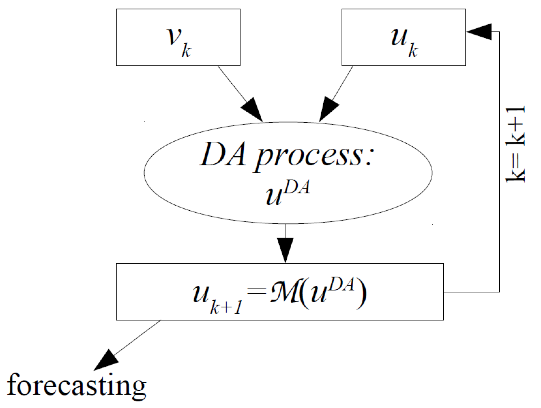
(called analysis) as an optimal tradeoff between the prediction made based on the estimated system state (called background) and the available observation. The state
u is then replaced by the function
, which includes the information from the observation
v in a prediction-correction cycle that is shown in
Figure 1.
The analysis
is computed as inverse solution of
subject to the constraint that
where
and
denote the observation error and model error, respectively,
denotes Gaussian distribution [
1], and
includes the measurement error
introduced in (
2). Both of the errors include the discretization, approximation and the other numerical errors.
Because
H is typically rank deficient, the (
5) is an ill posed inverse problem [
36,
37]. The Tikhonov formulation [
38] leads to an unconstrained least square problem, where the term in (
6) ensures the existence of a unique solution of the (
5). The DA process can be then described in Algorithm 1, where:
where
and
are the observation and model error covariance matrices, respectively:
with
and
I be the identity matrix,
with
background error deviation matrix [
13] being computed by a set of
historical data
available at time
and such that
where
and
| Algorithm 1 DA |
 |
The DA process, as defined in (
7), can be solved by several methods. Two main approaches that have gained acceptance as powerful methods for data assimilation on the last years are the variational approach and Kalman Filter (KF). The variational approach [
39] is based on the minimization of a functional, which estimates the discrepancy between numerical results and measures. The Kalman Filter [
40] is a recursive filtering instead. In both cases we seek an optimal solution. Statistically, KF seeks a solution with minimum variance. Variational methods seek a solution that minimizes a suitable cost function. In certain cases, the two approaches are identical and they provide exactly the same solution [
1]. However, the statistical approach, though often complex and time-consuming, can provide a richer information structure, i.e., an average and some characteristics of its variability (probability distribution).
Assuming the acquisition of the observations in a fixed time steps, the variational approach is named 3DVar [
1,
6], and it consists in computing the minimum of the cost function:
where
Potential problems of a variational method are mainly given by three main points: it heavily relies on correct matrices, it does not take system evolution into account, and it can end up in local minima.
Kalman Filter consists in computing the explicit solution of the normal equations:
where the matrix
is called Kalman gain matrix and where
is updated at each time step [
6]:
A potential problem of Kalman Filter is that is too large to store for large- dimensional problems.
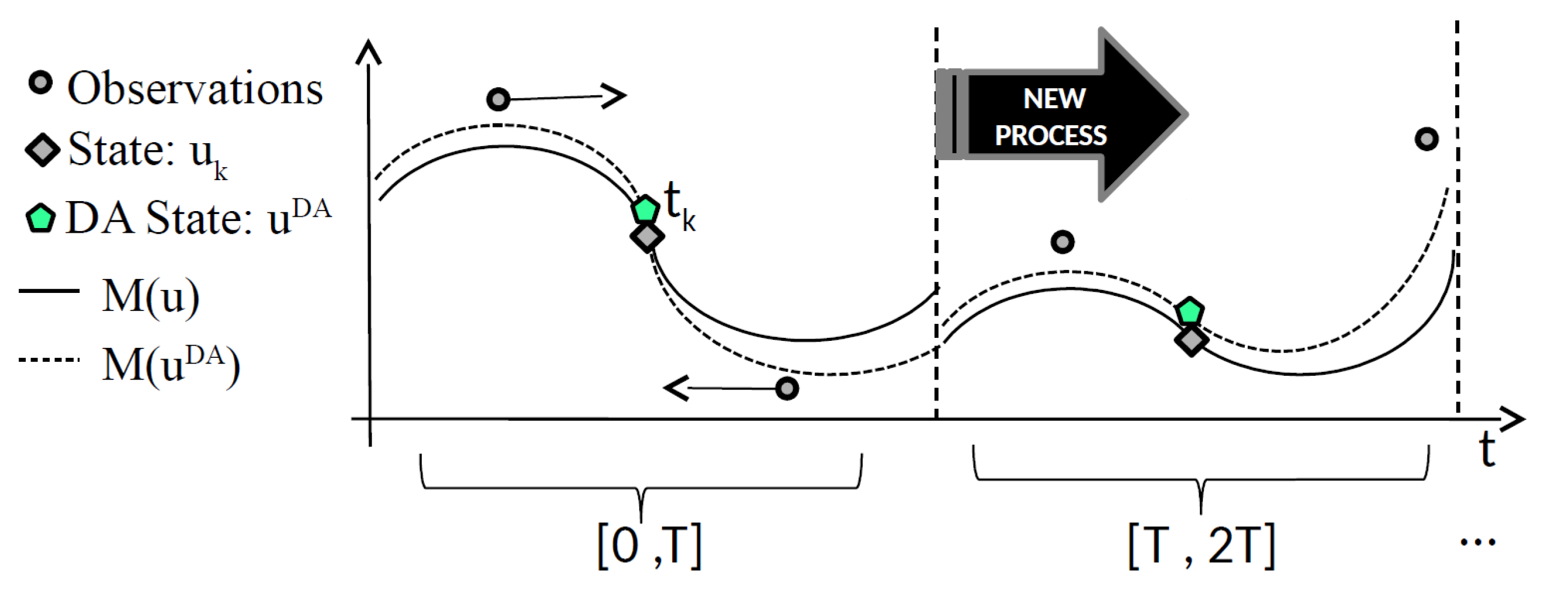
A common point of 3DVar and KF is that the observations that are defined in the window
(circle points in
Figure 2) are assimilated in the temporal point, where the state is defined (grey rhombus in
Figure 2 at time
). After the assimilation, a new temporal window
is considered and new observations are assimilated. Each process starts at the end point of the previous process and the two assimilation processes are defined in almost independent temporal windows. The result of the assimilation process
(green pentagons in
Figure 2), as computed by 3DVar or KF, is called analysis. The explicit expression for the analysis error covariance matrix, denoted as
, is [
1]:
where
I denotes the identity matrix.
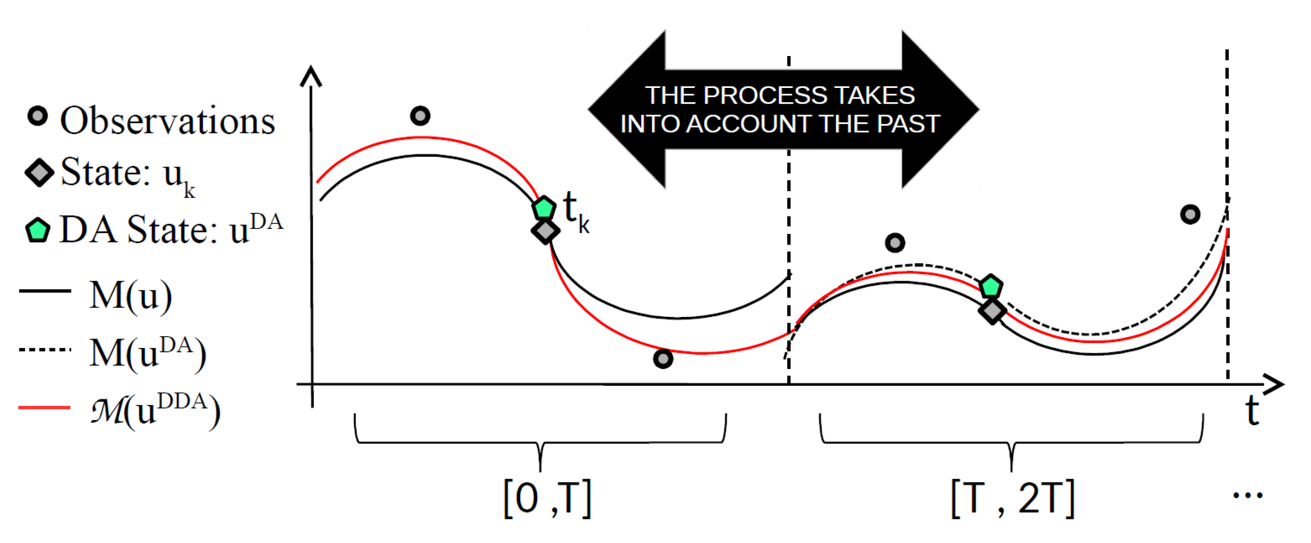
Even if the DA process takes information in a temporal window into account, it does not really take the past into account. This is due to the complexity of the real application forecasting models for which a long time window would be too computationally expensive. In next section, we introduce the Deep Data Assimilation (DDA) model, in which we replace the forecasting model
M (black line in
Figure 3) with a new Machine Learning model
(red line in
Figure 3) trained while using DA results and taking the past into account.
3. The Deep Data Assimilation (DDA) Model
Data assimilation (DA) methodologies improve the levels of confidence in computational predictions (i.e., improve numerical forecasted results) by incorporating observational data into a prediction model. However, the error propagation into the forecating model is not improved by DA, so that, at each step, correction have to be based from scratch without learning from previous experience of error correction. The strongly nonlinear character of many physical processes of interest can result in the dramatic amplification of even small uncertainties in the input, so that they produce large uncertainties in the system behavior [
5]. Because this instability, as many observations are assimilated as possible to the point where a strong requirement to DA is to enable real-time utilization of data to improve predictions. Therefore, it is desirable to use machine learning method in order to learn a function which accumulates the process of previous assimilation process. We use NN to model this process. The key concept is in recording each step of state correction during an assimilation period and then learn a function in order to capture this updating mechanism. The system model is then revised by composing this learned updating function with the current system model. Such a process continues by further learning the assimilation process with the updated system model.
The resulting NN-forecasting model is then a forecasting model with an intrinsic assimilation process.
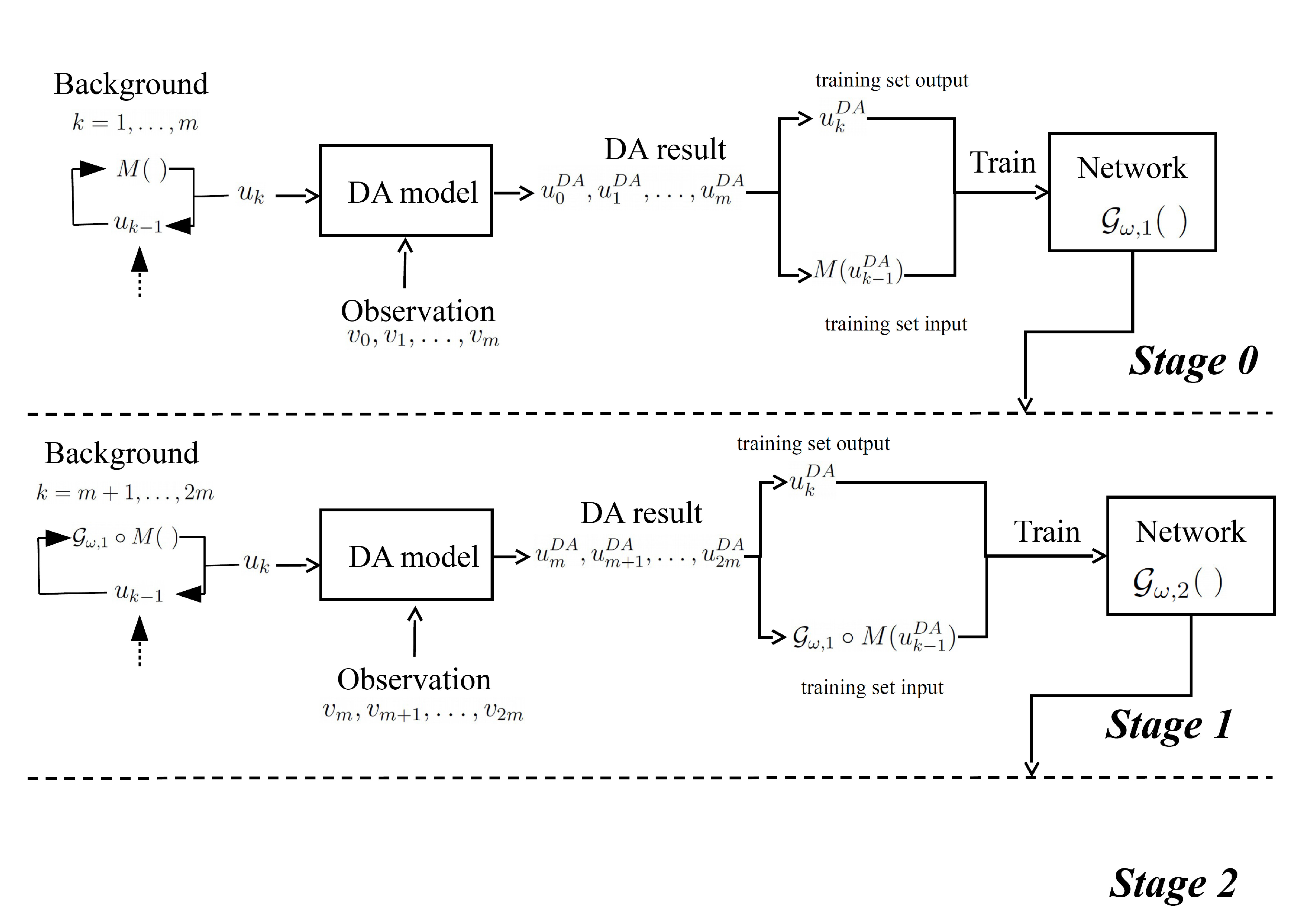
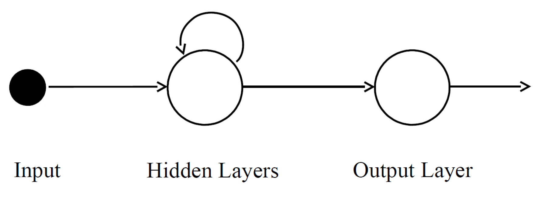
We introduce a neural network
, starting by a composition with the model
M, as described in
Figure 4. The training target is:
We train
by exploiting the results of DA, as described in Algorithm 2. The
model can be the iterative form
, where
is defined as the network that was trained in
ith iteration and
denotes the composition function. Let
be the model that was implemented in the
ith iteration, it is:
from which
, and
.
For iteration
, the training set for
is
, which exploits the
from the last updated model
. In this paper, we implement a Recurrent Neural Network (RNN) based on Elman networks [
41]. It is a basic RNN structure that loops through the hidden layer output as an internal variable (that corresponds to the Jordan network [
42] that outputs
as a variable). As shown in
Figure 5, the RNN is specifically expressed as
| Algorithm 2 |
 |
This choice to train the NN using data from DA introduces a reduction of the model’s error at each time step that can be quantified as reduction of the background error covariance matrix, as proved in next theorem.
Theorem 1. Let and be the error covariance matrices at step and step k in Algorithm 2, respectively. We prove that i.e., the error in background data is reduced at each iteration.
Proof. We prove the thesis by a reductio ad absurdum. We assume
At step
, from Step 10 of Algorithm 2 we have
, i.e., from (
15) and (
13), the (
21) gives
i.e., from the property of
:
, we have
which means that
Becaue of the definition of
, we can then assume that
, such that
i.e., such that
which is absurd. In fact, if we consider the two possible conditions
and
. In case
,
and
are diagonal elements of the errors covariance matrices. In other words, they are values of variances that mean that they are positive values and the (
26) is not satisfied. In case
,
as the error covariance matrix
is diagonal, as defined in (
8). Subsequently, we have that
and the (
26) is also not satisfied. Subsequently, the (
20) is proven. □
Another important aspect is that the solution of the DDA Algorithm 2 is more accurate than the solution of a standard DA Algorithm 1.
In fact, even if some sources of errors cannot be ignored (i.e., the round off error), then the introduction of the DDA method reduces the error in the numerical forecasting model (below denoted as ). The following result held.
Theorem 2. Let denote the error in the DA solution: and let be the error in DDA solution: Proof. Let
be error in the solution of the dynamic system M in (
3), i.e.,
. From the backward error analysis that was applied to the DA algorithm [
13], we have:
and
where
and
denote the condition numbers of the DA numerical model and the DDA numerical model, respectively.
It has been proved, in [
37], that the condition number of the DA and DDA numerical models are directly proportional to the condition numbers of the related background error covariance matrices
. Subsequently, thanks to the (
20), we have
, from which:
□
The DDA framework in this article implement a Recurrent neural network (RNN) structure as
. The loss function is defined, as described in Theorem 3 and the network is updated at each step by the gradient loss function on its weights and parameters:
Theorem 3. Let be the training set for , which exploits the data from the past updated model in (17). The loss function for the Back-propagation, being defined as mean square error (MSE) for the DA training set, is such thatwhere is the misfit between observed data and background data, and is the Hessian of the DA system. Prof. The mean square error (MSE)-based loss function for the Back-propagation is such that
The solution
of the DDA system, which is obtained by a DA function, can be expresses as [
1]:
Let posed
and
, (
34) gives:
Substituting, in (
33), the expression of
given by (
35), the (
32) is proven. □
4. Experiments
In this section, we apply the DDA technology to two different applications: the Double integral mass dot system and the Lorenz system:
Double integral mass dot system:
For the physical representation of a generalized motion system, the double-integral particle system is commonly used. The method, under the influence of an acceleration regulation quantity, can be seen as the motion of a particle. The position and velocity are the variables that affect the state at each time step. The status as a controlled state gradually converges to a relatively stable value, due to the presence of a PID controller in the feedback control system. The performance of the controller is the system-acting acceleration, or it can be interpreted as a force that linearly relates to the acceleration.
Double integral system is a mathematic abstraction of Newton’s Second Law that is often used as a simplified model of several controlled systems. It can be represented as a continuous model, as:
where the state
is a two-dimensional vector containing position
and velocity
and where
is the controlled input. The coefficients matrices
A,
B, and
C are time-invariant system and observations matrices.
r is the noise of the observations, which is Gaussian and two dimensional. The system disruption
comprises two aspects: random system noise and instability of the structural model.
Lorenz system:
Lorenz developed a simplified mathematical model for atmospheric convection in 1963. It is a common test case for DA algorithms. The model is a system of three ordinary differential equations, named Lorenz equations. For some parameter values and initial conditions, it is noteworthy for having a chaotic behavior. The Lorenz equations are given by the nonlinear system:
where
p,
q and
r are coordinates, and
,
, and
are parameters. In our implementation, the model has been discretized by second order Runge–Kutta method [
43] and, for this test case, we posed
,
and
.
We mainly provide testing in order to validate the results that we proved in the previous section. Afterwards, we mainly focus on:
- 4.1
DDA accuracy: we prove that the accuracy of the forecasting result increases as the number of time steps increases, as proved in Theorem 1;
- 4.2
DDA vs. DA: in order to address the true models, we face the circumstances where DA is not sufficient to reduce the modeling uncertainty and we show that the DDA algorithm, we have proposed is applicable to solve this issue. Such findings validate what we showed in Theorem 2; and,
- 4.3
R-DDA vs. F-DDA: we are demonstrating that the accuracy of the R-DDA is better than that of the F-DDA. It is also due to the way the weight is calculated, i.e., by including the DA covariance matrices, as shown in Theorem 3.
We implemented the algorithms on the Simulink (Simulation and Model-Based Design) in Matlab 2016a.
4.1. DDA Accuracy
4.1.1. Double Integral Mass Dot System
When considering model uncertainty, a system disturbance in (
36) is introduced so that:
where
denotes the structural model uncertainty and
denotes the i.i.d random disturbance.
One typical model error is from the parallel composition as:
where the amplitude vector
is adjustable, according to the reality.
A cascade controller is designed to prevent divergence from the device in order to accomplish the model simulation. As a sinusoidal function, the tracking signal is set. 10,000 samples are collected from a 100 s simulation with a 100 Hz sample frequency. The training set for the DDA Algorithm 2 is made of the time series
of
m couples. First of all, we run the framework for the dynamic system Equation (
36) and record the observation
v, control input
z. A corresponding DA runs alongside program updates, and outputs a
prediction sequence. The network
is trained on the dataset of
m steps.
Subsequently, the system and the DA update the data from the
step to
step. Although the device upgrade process in DA now incorporates the qualified neural network
, as:
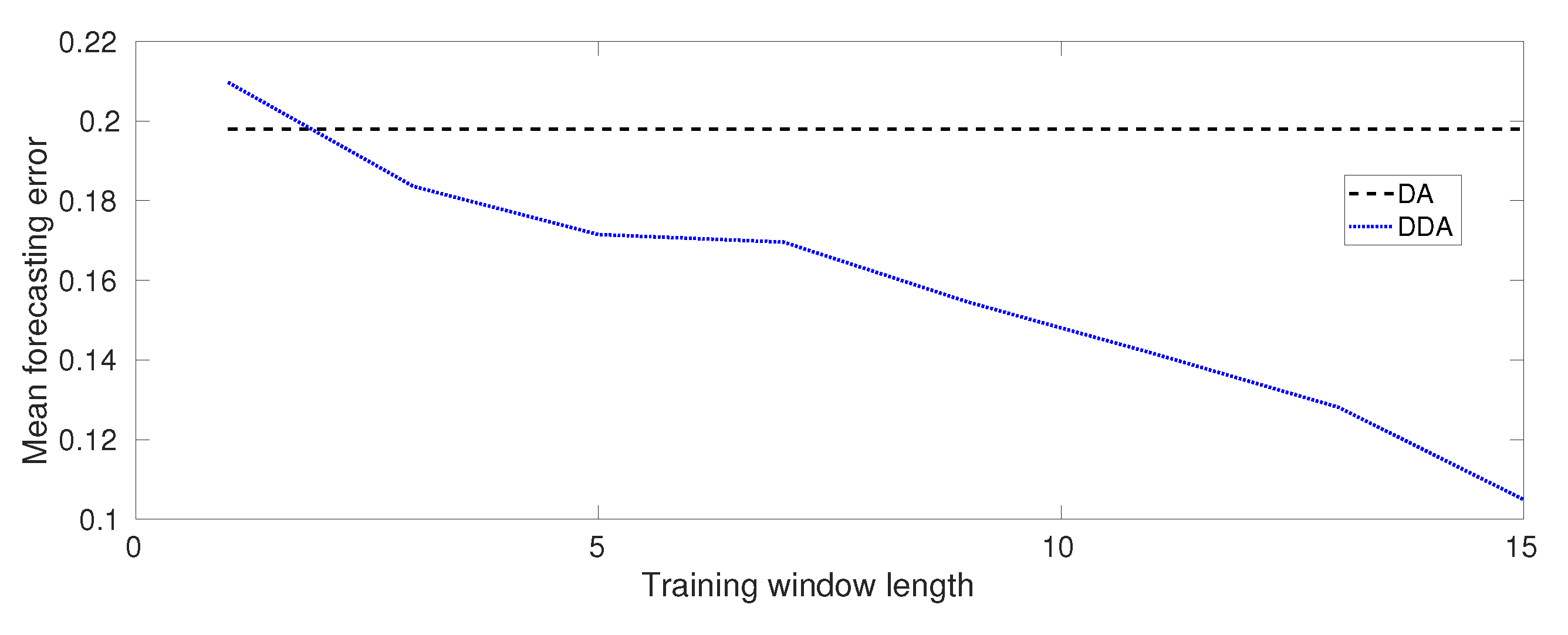
Figure 6 shows what we expected regarding the accuracy of DDA. In fact, as it is shown, the mean forecasting error decrease as the training window length increases. The Figure also shows a comparison of the mean forecasting error values with respect the results that were obtained from DA.
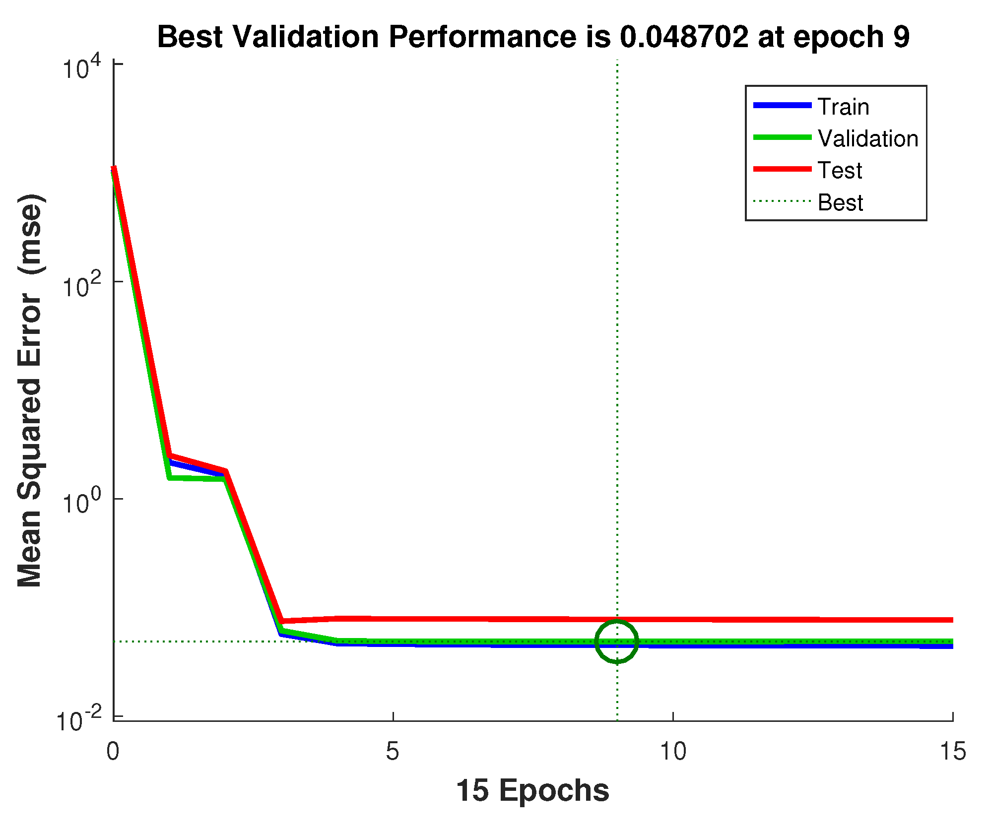
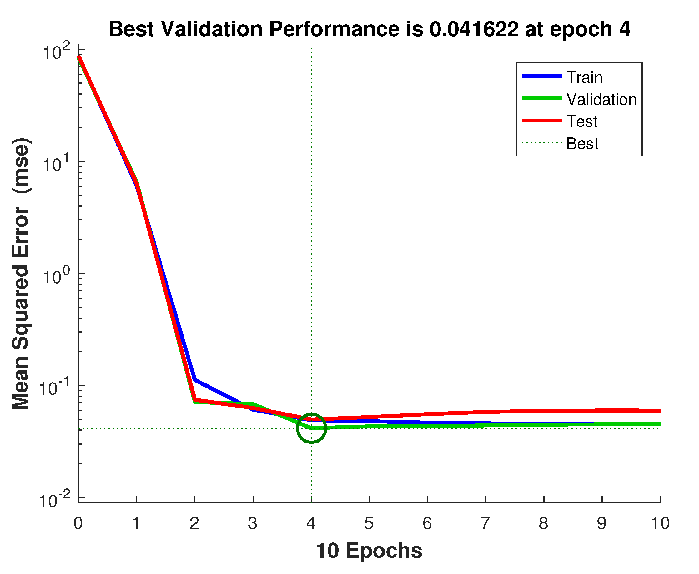
Figure 7 is a convergence curve when matlab trains a network using the Levenberg–Marquardt backpropagation [
44,
45] method. It can be seen that, with just few epochs, the best value for the mean square error is achieved.
4.1.2. Lorenz System
We implement a Lorenz system with structural model uncertain as:
where
denotes the state and
denotes the discrete function. The structural model uncertainty is denoted here as
, with
, and
, such that:
First of all, for the dynamic system, Equation (
37), we run the system and record the true value of the system
u. Subsequently, by adding Gaussian noise to the true value of
u,
v is created. The DA algorithm is then applied to produce a sequence with a DA result of
and a length of
m. The training set is made of the time series
. Afterwards, the neural network
is trained.
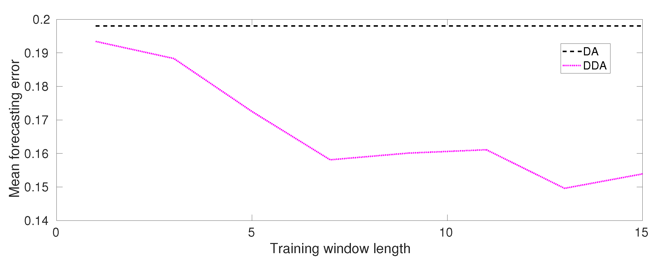
Figure 8 shows the accuracy results of DDA for Lorenz test case. Additionally, in this case, the results confirm our expectation. In fact, as it is shown, the mean forecasting error decrease as the training window length increases. Additionally, in this figure, a comparison of the mean forecasting error values with respect the results obtained from DA is shown.
Figure 9 is a convergence curve when matlab trains a network using the Levenberg–Marquardt backpropagation method and, also in this case, the best value for the mean square error is achieved with just a few epochs.
4.2. DDA vs. DA
In this section, we compare the forecasting results based on DA model and the DDA model, respectively. For the DA, the system model update is formed as:
where
is the discrete forecasting system in (
3). For DDA, the system update model is as:
where
is defined in (
17).
4.2.1. Double Integral Mass Dot System
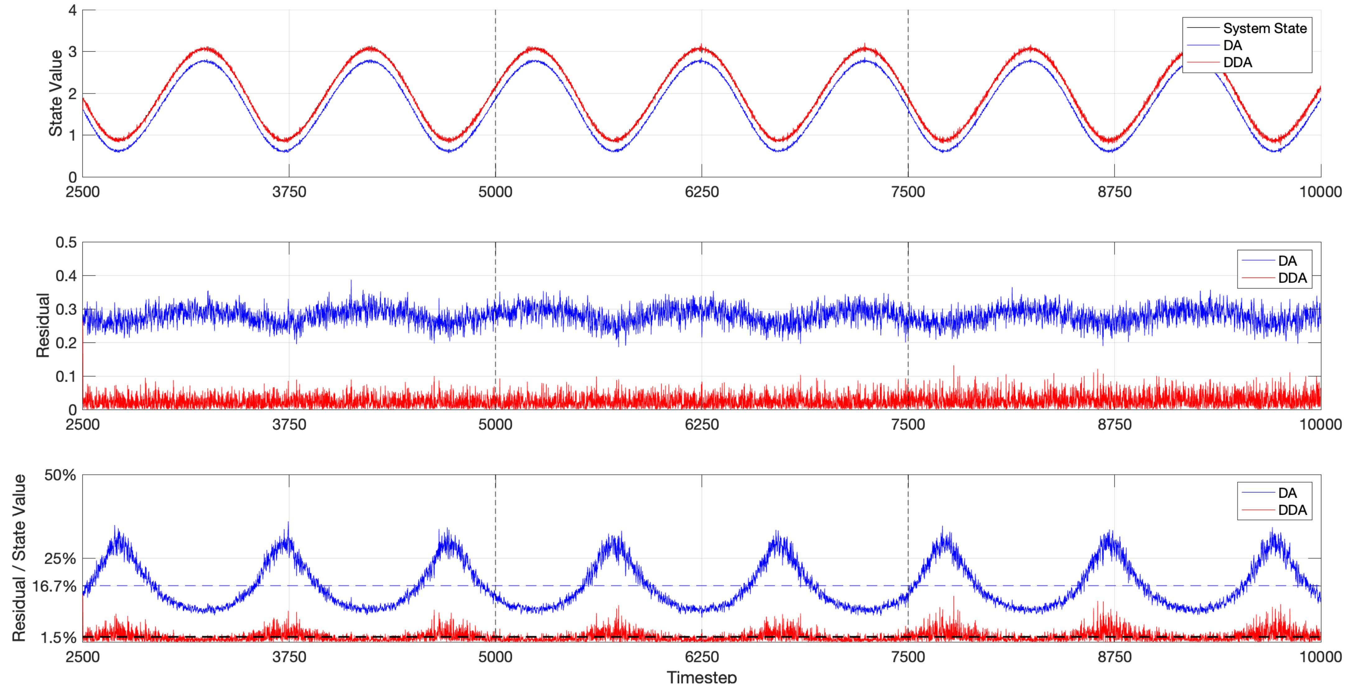
Figure 10 shows the result of DA and DDA model on a double integral system that considers the model error. Two vertical dash lines are at which the neural network is trained. Obviously, the forecasting state value based on DDA is more closer to the true value than DA. The DA results in a larger residual. We also calculate the ratio of residual to true value as a forecasting error metric. The average forecasting error is significantly reduced from 16.7% to 1.5% by applying DDA model.
Table 1 lists the run-time cost of every training window in
Figure 10.
4.2.2. Lorenz System
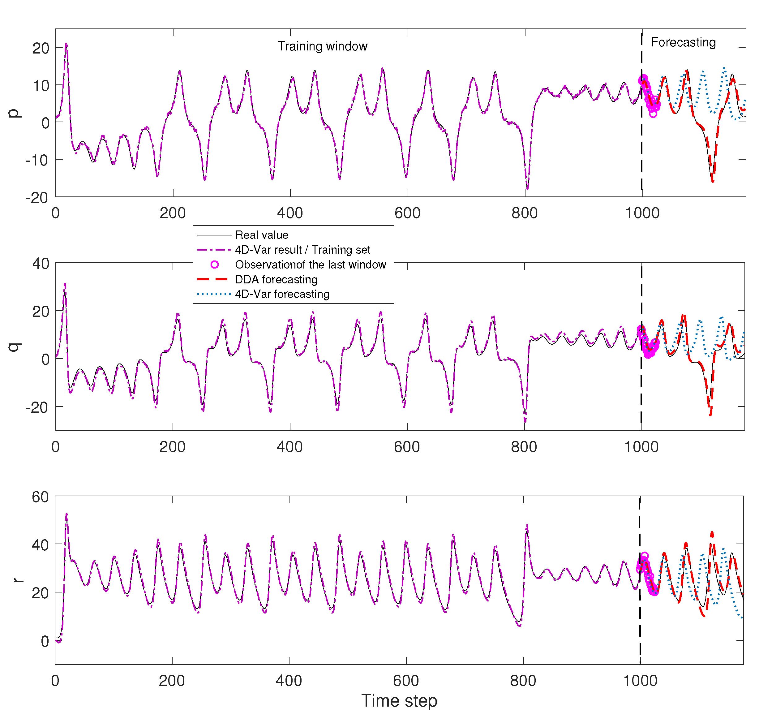
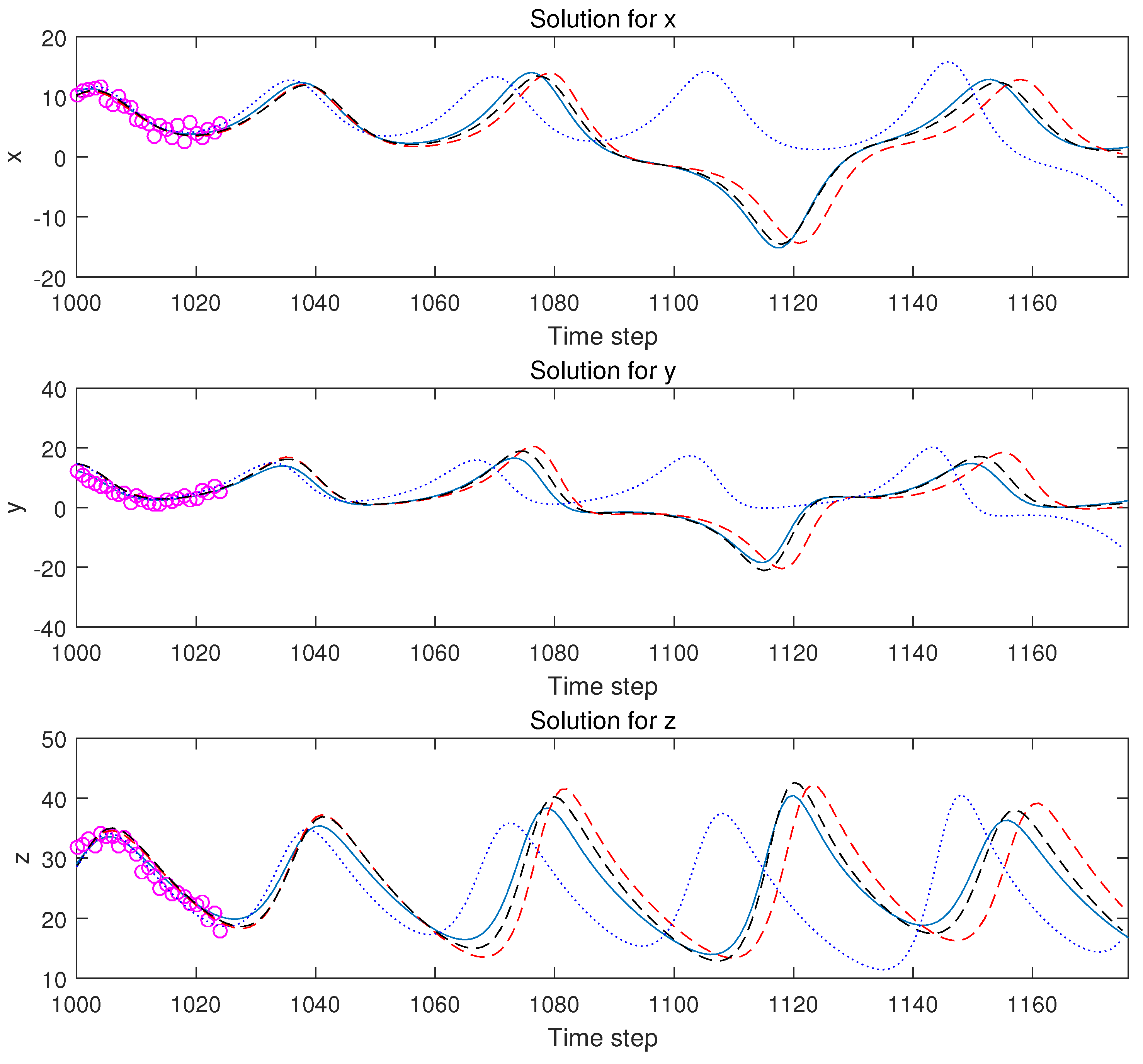
We compare the forecasting results that are shown in
Figure 11. The
generated training set is not plotted in full. The forecast starts at
. We can see that the DA model’s forecasting errors in all three axes are large. DA model trajectories can not track the real state. Although the DDA model trajectories track the true value very well.
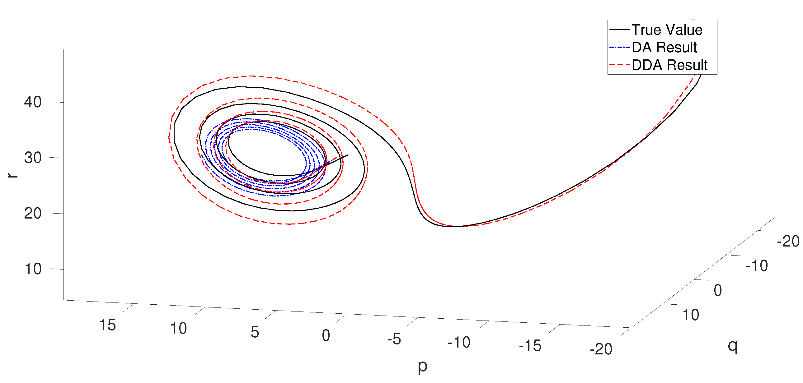
Figure 12 is a 3D plot of this forecasting part of the Lorenz system. This demonstrates that the DA model fails to predict the right hand part of this butterfly. In this test, for the right wing trajectory of butterfly, the DDA model outperforms the DA model in forecasting.
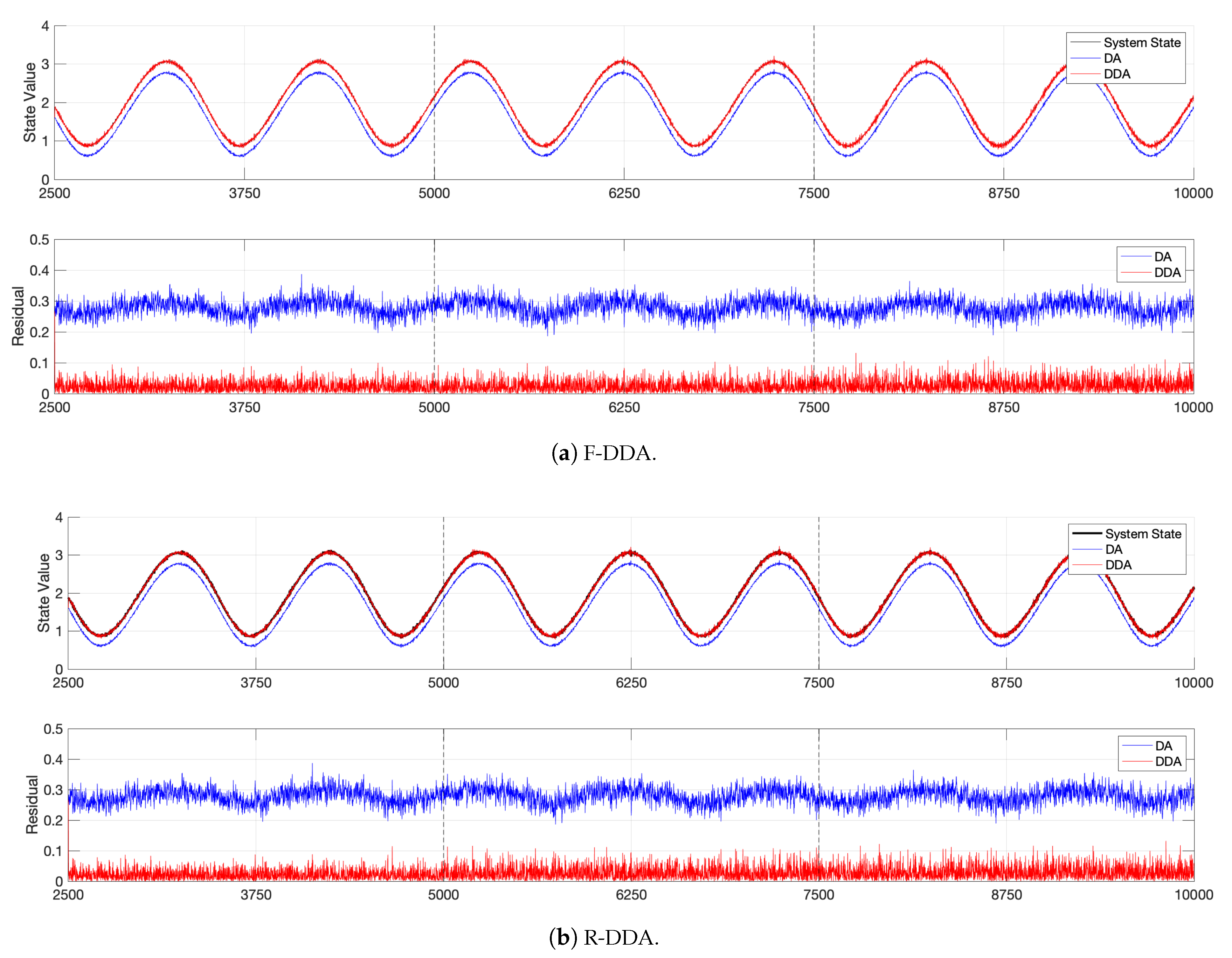
4.3. F-DDA vs. R-DDA
In this section, we introduce the DDA using the feedfoward neural network (we named F-DDA) and compare the results with the R-DDA, i.e., the DDA we described in this paper that uses the recurrent neural network. The feed-foward (FC) network is the earliest and most basic neural network structure. This means that in the next layer, the output of each neuron in the upper layer becomes the input of each neuron, and it has a structure with corresponding values of weight. Inside the FC network, there is no cycle or loop. In the fitting of functions, fully conected neural networks are widely cited (especially the output of continuous value functions). The multilayer perceptron (MLP), which contains three hidden layers, is used in this paper.
In the training step of the DDA framework, the training set is the DDA result over a period of time. Take the first cycle () as an example. The training set is (the results of consecutive time series), and this data set generates the model. Because this network is a feedfoward neural network and it is unable to manage time series, we consider that the training set for the M category is independent of each other.
4.3.1. Double Integral Mass Dot System
In this section, we compared the performance of F-DDA and R-DDA in the double integral mass dot system. Because our data were previously generated by simulink, random noise, and observation noise are fixed and can be compared.
Figure 13 shows that F-DDA obtains a similar result when comparing to R-DDA in this case. It is mainly because the double integral mass dot system is not strongly dependent on the time historical states. Meanwhile, when considering the execution time cost that is shown in
Table 1, F-DDA is more preferable, as it takes shorter training time than R-DDA.
4.3.2. Lorenz System
Figure 14 is a comparison of the forecasting results of F-DDA and R-DDA for the Lorenz system. It can be seen that the R-DDA (black dashed line) has a more accurate prediction of the true value (blue solid line) and the curve fits better. In contrast, F-DDA (red dotted line) has a certain time lag and it is also relatively inaccurate in amplitude. This is mainly because the Lorenz system is strongly time-dependent.
Table 2 provides the run-time cost for both F-DDA and R-DDA in training and forecasting. It is worth taking more training time for R-DDA to achieve a better prediction than F-DDA.
5. Conclusions and Future Work
In this article, we discuss the DDA: the integration of DL and DA and we validate the algorithm by a numerical examples. The DA methods have increased strongly in complexity in order to better suit their application requirements and circumvent their implementation problems. However, the approaches to DA are unable to fully overcome their unrealistic assumptions, particularly of zero error covariances, linearity, and normality. DL shows great capability in approximating nonlinear systems, and extracting high-dimensional features. Together with the DA methods, DL is capable of helping traditional methods to make forecasts without the conventional methods’ assumptions. On the other side, the training data provided to DL technologies include several numerical, approximation, and round off errors that are trained in the DL forecasting model. DA can increase the reliability of the DL models reducing errors by including information on physical meanings from the observed data.
This paper showed that the cohesion of DL and DA is blended in the future generation of technology that is used in support of predictive models.
So far, the DDA algorithm still remains to be implemented and verified in varies specific domains, which have huge state space and more complex internal and external mechanisms. Future work includes adding more data to the systems. A generalization of DDA could be developed if it is used for different dynamical systems.
The numerical solution of dynamic systems could be replaced by DL algorithms, such as Generative Adversarial Networks or Convolutional Neural Networks combined with LSTM, in order to make the runs faster. This will accelerate the forecast process towards a solution in real time. When combined with DDA, this future work has the potential to be very fast.
DDA is encouraging, as speed and accuracy are typically terms that are mutually exclusive. The results that are shown here are promising and demonstrate how, in computationally demanding physical models, the merger of DA and ML models, especially in computationally demanding physical models.


