Classification of Objects by Shape Applied to Amber Gemstone Classification

 ,
,  and
and
Abstract
1. Introduction and Related Work
2. Proposed Methodology
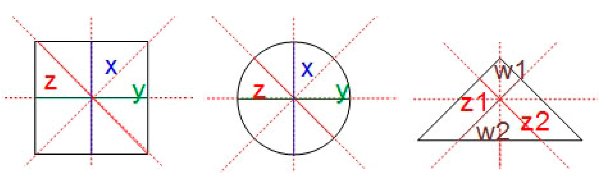
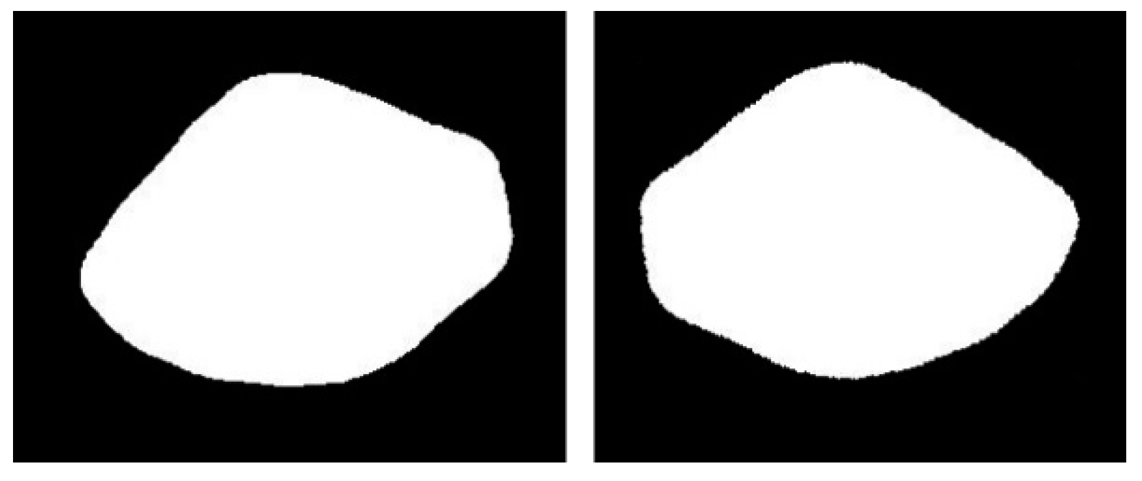
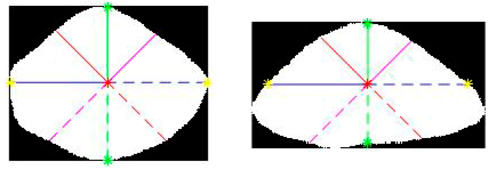
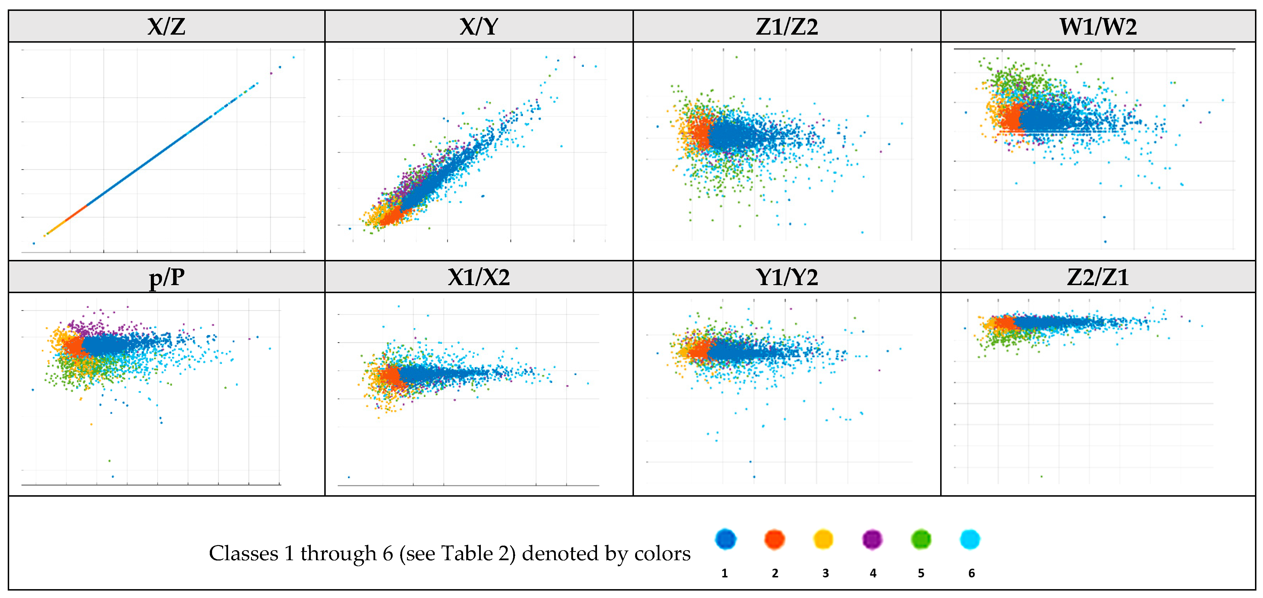
2.1. Shape Parametric Description
| Code 1 |
| Pseudocode for the form identification algorithm. Herein, tol1 and tol2 refer to the tolerance values (allowed parameter deviation limits), P is the area of the rectangle limiting the object’s shape (P = x ∗ y), and p is the real area of the investigated object in pixels. IF Z1/Z2 < 1 − tol1 OR 1 + tol1 < Z1/Z2 THEN triangle form check ELSEIF W1/Z2 < 1 − tol1 OR 1 + tol1 < W1/Z2 THEN Asymmetrical form ELSEIF 1 − tol1 < X/Y AND X/Y < 1 + tol1 THEN symmetric proportional form check ELSEIF X/Y > 1 + tol1 THEN symmetric nonproportional form checking; END IF |
| Code 2 |
| Pseudocode for checking triangle forms. IF X/Y < 1 − tol1 THEN Isosceles triangle ELSEIF X/Y > 1 − tol1 THEN Right triangle ELSE THEN Equilateral triangle END IF |
| Code 3 |
| Pseudocode for checking proportional symmetric forms. IF p/P < 1 − tol1 THEN Circle ELSE THEN Square END IF |
| Code 4 |
| Pseudocode for checking nonproportional symmetric forms. IF p/P > 1 − tol1 AND X/Z < 1 − tol2 THEN Asymmetrical form ELSEIF p/P > 1 − tol2 AND X/Z > 1 + tol1 THEN Rectangle ELSEIF p/P < 1 − tol1 AND X/Z > 1 + tol1 THEN Oval END IF |
2.2. Machine Learning Algorithms
3. Experiments and Results
3.1. Hardware and Implementation
3.2. Preprocessing
3.3. Experimental Results for the SPD and CDF Approaches
3.4. Experimental Results after Applying Machine Learning
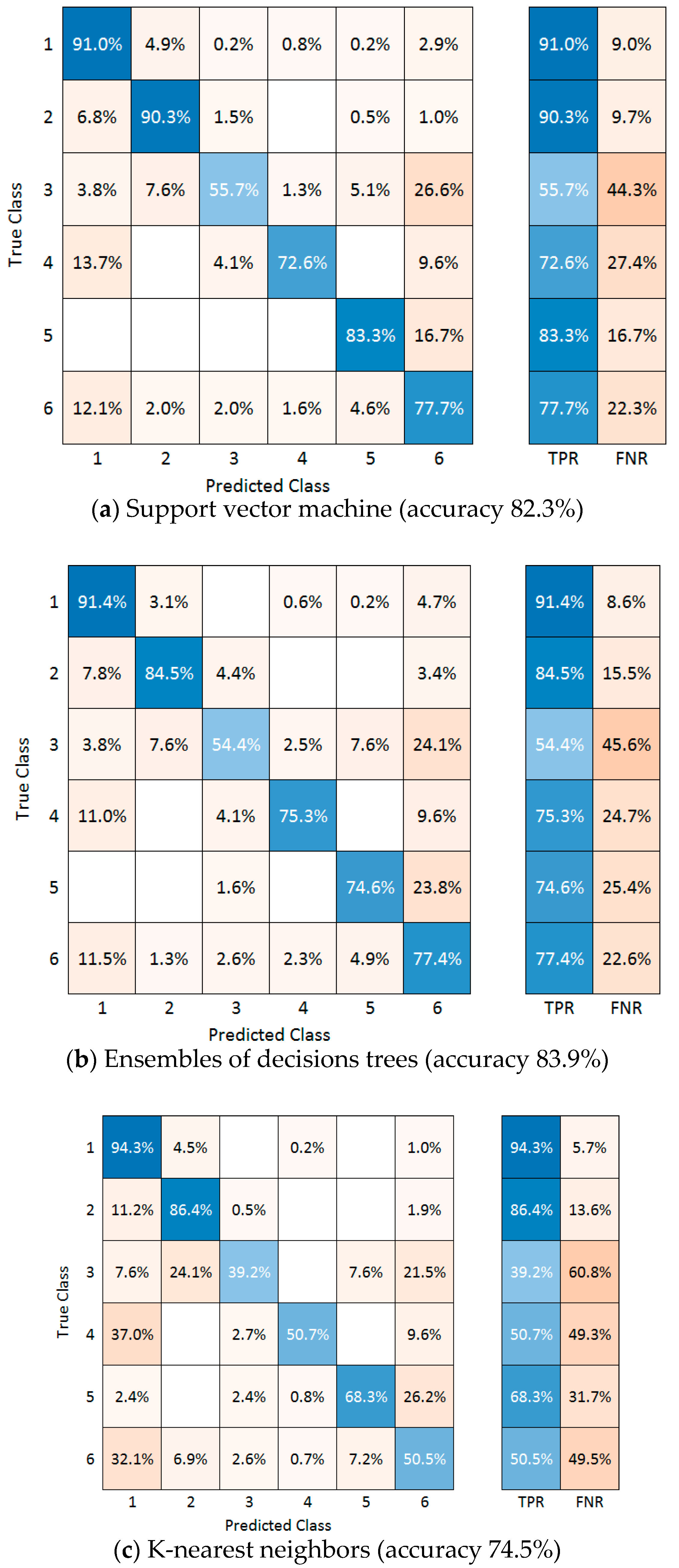
3.5. Classification Performance
4. Conclusions
Author Contributions
Funding
Institutional Review Board Statement
Informed Consent Statement
Conflicts of Interest
References
- Lorencs, A.; Mednieks, I.; Sinica-Sinavskis, J. Simplified Classification of Multispectral Image Fragments. Elektron. Elektrotech. 2014, 20, 136–139. [Google Scholar] [CrossRef]
- Pearson, T.; Moore, D.; A Pearson, J.R. A machine vision system for high speed sorting of small spots on grains. J. Food Meas. Charact. 2012, 6, 27–34. [Google Scholar] [CrossRef]
- Shahrani, S.; Aini, H.; Dzuraidah, A.W.; Mohd, M.M.; Suzaimah, R. Support vector machines for automated classification of plastic bottles. In Proceedings of the 6th International Colloquium Signal Processing and Its Applications (CSPA), Melaka, Malaysia, 21–23 May 2010; pp. 1–5. [Google Scholar] [CrossRef]
- O’Farrell, M.; Lewis, E.; Flanagan, C.; Lyons, W.B.; Jackman, N. Design of a system that uses optical-fiber sensors and neural networks to control a large-scale industrial oven by monitoring the food quality online. IEEE Sens. J. 2005, 5, 1407–1420. [Google Scholar] [CrossRef]
- Pearson, T.; Brabec, D.; Haley, S. Color image based sorter for separating red and white wheat. Sens. Instrum. Food Qual. Saf. 2008, 2, 280–288. [Google Scholar] [CrossRef]
- Sinkevičius, S.; Lipnickas, A.; Rimkus, K. Organic shapes classifications by similarity to basic geometric shapes. Int. J. Comput. Inf. Technol. 2014, 3, 503–507. [Google Scholar]
- Sinkevicius, S.; Lipnickas, A.; Rimkus, K. Automatic amber gemstones identification by color and shape visual properties. Eng. Appl. Artif. Intell. 2015, 37, 258–267. [Google Scholar] [CrossRef]
- Jorge, J.; Fonseca, M.J. A Simple Approach to Recognise Geometric Shapes Interactively. Available online: web.tecnico.ulisboa.pt/~jorgej/papers/grec99.pdf (accessed on 5 November 2020).
- Bochkarev, S.O.; Litus, I.B.; Kravchenko, N.S. Irregular Objects. Shape Detection and Characteristic Sizes. Available online: Ceur-ws.org/Vol-1814/paper-04.pdf (accessed on 5 November 2020).
- Mazzeo, P.L.; Argentieri, A.; De Luca, F.; Spagnolo, P.; Distante, D.; Leo, M.; Carcagnì, P. Convolutional neural networks for recognition and segmentation of aluminum profiles. In Proceedings of the SPIE 11059, Multimodal Sensing: Technologies and Applications, 110590S, Munich, Germany, 21 June 2019. [Google Scholar]
- Sarstedt, M.; Mooi, E. Concise Guide to Market Research, 2nd ed.; Springer: Berlin/Heidelberg, Germany, 2014; ISBN 978-3-642-53965-7. [Google Scholar] [CrossRef]
- Sinkevicius, S.; Lipnickas, A.; Rimkus, K. Multiclass amber gemstones classification with various segmentation and committee strategies. In Proceedings of the IEEE 7th International Conference on Intelligent Data Acquisition and Advanced Computing Systems (IDAACS), Berlin, Germany, 12–14 September 2013; Available online: https://ieeexplore.ieee.org/document/6662694 (accessed on 5 November 2020). [CrossRef]
- Sinkevicius, S.; Lipnickas, A.; Rimkus, K. Amber Gemstones Sorting by Colour. Elektron. Elektrotech. 2017, 23, 10–14. [Google Scholar] [CrossRef]


| Class | Correct | Incorrect | Accuracy |
|---|---|---|---|
| 1. Oval | 1437 | 305 | 82.5% |
| 2. Circle | 563 | 138 | 80.3% |
| 3. Rectangle | 185 | 80 | 69.8% |
| 4. Square | 173 | 74 | 70.0% |
| 5. Triangle | 321 | 104 | 75.5% |
| 6. Asymmetrical | 780 | 251 | 75.7% |
| Total | 3459 | 952 | 78.4% |
| Class | Correct | Incorrect | Accuracy |
|---|---|---|---|
| 1. Oval | 1437 | 305 | 82.5% |
| 2. Circle | 503 | 198 | 71.8% |
| 3. Rectangle | 176 | 89 | 66.4% |
| 4. Square | 155 | 92 | 62.8% |
| 5. Triangle | 303 | 122 | 71.3% |
| 6. Asymmetrical | 753 | 278 | 73.0% |
| Total | 3267 | 1084 | 74.1% |
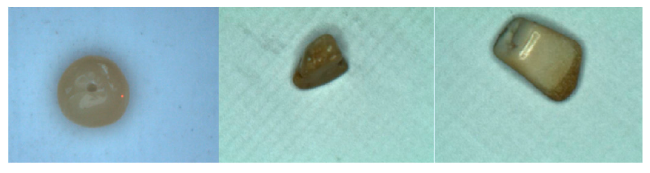
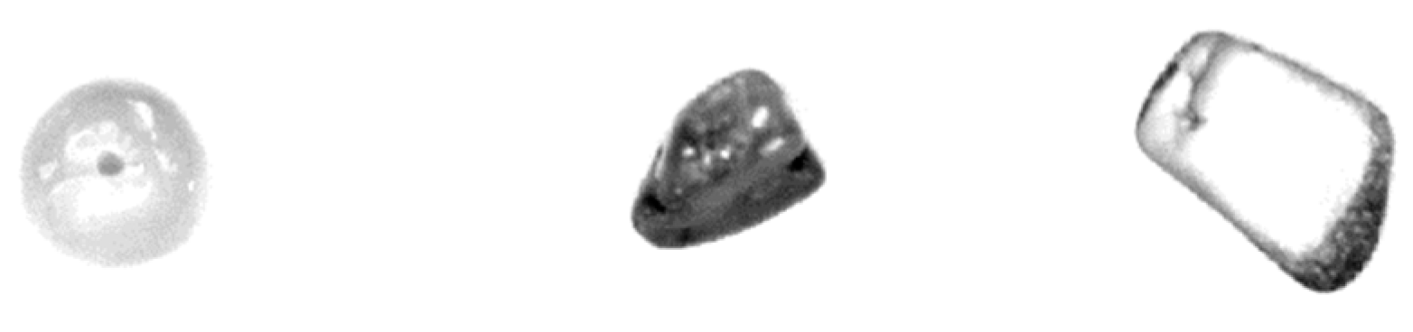
| Circle | Square | Triangle |
|---|---|---|
 |  |  |
| Form | SPD Method | CDF Method | ||
|---|---|---|---|---|
| Properly Identified Class | Incorrectly Identified Class | Properly Identified Class | Incorrectly Identified Class | |
| Circle | 3484 | 99 | 3619 | 101 |
| Square | 3277 | 100 | 3651 | 114 |
| Triangle | 3286 | 103 | 3610 | 110 |
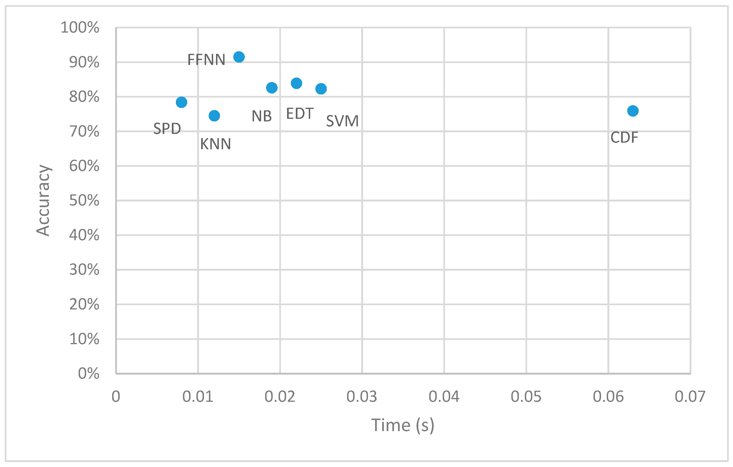
| Method | CDF | SVM | EDT | NB | FFNN | KNN | SPD |
|---|---|---|---|---|---|---|---|
| Time (s) | 0.063 | 0.025 | 0.022 | 0.019 | 0.015 | 0.012 | 0.008 |
| Accuracy | 75.9% | 82.3% | 83.9% | 82.6% | 91.5% | 74.5% | 78.4% |
| F1 macro-score | 0.62 | 0.74 | 0.76 | 0.77 | 0.89 | 0.66 | 0.73 |
| F1 micro-score | 0.86 | 0.90 | 0.91 | 0.90 | 0.96 | 0.85 | 0.88 |
Publisher’s Note: MDPI stays neutral with regard to jurisdictional claims in published maps and institutional affiliations. |
© 2021 by the authors. Licensee MDPI, Basel, Switzerland. This article is an open access article distributed under the terms and conditions of the Creative Commons Attribution (CC BY) license (http://creativecommons.org/licenses/by/4.0/).
Share and Cite
Ostreika, A.; Pivoras, M.; Misevičius, A.; Skersys, T.; Paulauskas, L. Classification of Objects by Shape Applied to Amber Gemstone Classification. Appl. Sci. 2021, 11, 1024. https://doi.org/10.3390/app11031024
Ostreika A, Pivoras M, Misevičius A, Skersys T, Paulauskas L. Classification of Objects by Shape Applied to Amber Gemstone Classification. Applied Sciences. 2021; 11(3):1024. https://doi.org/10.3390/app11031024
Chicago/Turabian StyleOstreika, Armantas, Marius Pivoras, Alfonsas Misevičius, Tomas Skersys, and Linas Paulauskas. 2021. "Classification of Objects by Shape Applied to Amber Gemstone Classification" Applied Sciences 11, no. 3: 1024. https://doi.org/10.3390/app11031024
APA StyleOstreika, A., Pivoras, M., Misevičius, A., Skersys, T., & Paulauskas, L. (2021). Classification of Objects by Shape Applied to Amber Gemstone Classification. Applied Sciences, 11(3), 1024. https://doi.org/10.3390/app11031024