Review

Rigidity through a Projective Lens

1
Department of Mathematics and Statistics, Lancaster University, Lancaster LA1 4YF, UK
2
Deptartment of Mathematics and Statistics, York University, Toronto, ON M3J 1P3, Canada
*
Author to whom correspondence should be addressed.
These authors contributed equally to this work.
Appl. Sci. 2021, 11(24), 11946; https://doi.org/10.3390/app112411946
Submission received: 16 April 2021 / Revised: 8 October 2021 / Accepted: 15 October 2021 / Published: 15 December 2021
(This article belongs to the Special Issue New Applications of (Old School) Projective Geometry)

Abstract

:

Featured Application

The material in this article draws on, and has applications across a range of applications in civil and structural engineering, mechanical engineering, computer science, biochemistry, geometry and applied mathematics.

Abstract

In this paper, we offer an overview of a number of results on the static rigidity and infinitesimal rigidity of discrete structures which are embedded in projective geometric reasoning, representations, and transformations. Part I considers the fundamental case of a bar–joint framework in projective d-space and places particular emphasis on the projective invariance of infinitesimal rigidity, coning between dimensions, transfer to the spherical metric, slide joints and pure conditions for singular configurations. Part II extends the results, tools and concepts from Part I to additional types of rigid structures including body-bar, body–hinge and rod-bar frameworks, all drawing on projective representations, transformations and insights. Part III widens the lens to include the closely related cofactor matroids arising from multivariate splines, which also exhibit the projective invariance. These are another fundamental example of abstract rigidity matroids with deep analogies to rigidity. We conclude in Part IV with commentary on some nearby areas.

Contents
1.Introduction3
IProjective Geometry in Core Rigidity Results5
2.Introduction to Euclidean Rigidity Theory5
3.Projective Rigidity8
 3.1.Plücker Coordinates and Extensors8
 3.2.Infinitesimal and Static Rigidity in Projective Space10
 3.3.Projective Invariance 15
 3.4.Equivalence of Projective and Euclidean Rigidity Matrices16
4.Projective Metrics: Euclidean; Spherical; Hyperbolic; and Minkowski.17
 4.1.Euclidean and Spherical Spaces18
 4.2.Minkowski Space 20
5.Coning and Projecting21
 5.1.Coning a Framework from P d to P d + 1 21
 5.2.Coning and Projection for S d , M d , and H d 24
6.Joints at Infinity and Sliders25
 6.1.Point-Hyperplane Frameworks27
 6.2.Point-Hyperplane Frameworks and Projections from Spherical Frameworks27
 6.3.Sliders: Free and Pinned29
 6.4.Linear Constraints as Sliders31
 6.5.Further Extensions to Include Infinity 31
7.Pure Conditions32
 7.1.Bracket Ring32
 7.2.Small Examples 33
 7.3.Bipartite Frameworks and Quadratic Surfaces 35
 7.4.Pure Conditions: Basic Theorems39
 7.5.Factoring and Rigid Components 41
 7.6.Computing Pure Conditions: Pinned Frameworks, and d-Directed Graphs 43
 7.7.Assur Graphs and Assur Decompositions46
8.Polarity for Rigidity .50
 8.1.Duality and Polarity for Projective Geometry 51
 8.2.Sheet Structures and Polarity for Rigidity in R 3 51
 8.3.Substitution Principles56
 8.4.Cauchy, Alexandrov and Polarity57
IIProjective Theory of Connected Body Frameworks58
9.Body-Bar Frameworks58
 9.1.Body-Bar Combinatorics60
 9.2.Body-Bar Projective Conditions and Centers of Motion 63
 9.3.Projective Line Dependences and the Stewart Platform65
 9.4.Static Rigidity and Stresses in Body-Bar Frameworks67
 9.5.Coning Body-Bar Frameworks70
 9.6.Rod and Bar Frameworks in 3-Dimensions70
10.Body–Hinge Frameworks73
 10.1.Body–Hinge Basic Transfer73
 10.2.Body–Hinge Motion Assignments74
 10.3.Coning for Body–Hinge in P d 75
 10.4.Molecular and Body-Plate Frameworks 76
 10.5.Applications to Protein Structures 77
 10.6.Block and Hole Polyhedra79
 10.7.Lower Dimensional Bodies: Pinned Rods in the Plane83
 10.8.Summary Table 83
IIIMaximal Abstract Rigidity Matroids and Multivariate Splines84
11.Multivariate Splines and Cofactor Matroids85
 11.1.Smoothing Cofactors for Splines and Compatibility Conditions85
 11.2.The C 2 1 -Cofactor Matroid on Plane Graphs: An Analogue of Rigidity in P 3 87
 11.3. C 2 1 Is the Maximal Abstract 3-Rigidity Matroid87
 11.4.Transferring Pure Conditions 89
 11.5.Transferring Theorems to the C 2 1 -Cofactor Matroid 92
 11.6.Coning Splines: Abstract 4-Dimensional Rigidity Matroids and Multivariate Splines93
 11.7.Using Projective Rigidity Style Techniques for C d r 93
IVConcluding Connections94
12.Projective Tensegrities94
13.Further Explorations97
 13.1.Skeletal Rigidity, Geometric Homology and f-Vectors 97
 13.2.Global Rigidity, Universal Rigidity and Superstability 97
 13.3.Interesting However, Not Projective: Finite Motions 98
 13.4.Interesting However, Not Projective: CAD Constraints and Angles99
14.Companion Paper: Projective Geometry of Scene Analysis, Parallel Drawing and Reciprocal Drawing99
Backmatter 100
References100

1. Introduction

The study of the rigidity and flexibility properties of bar–joint structures can be traced back to work of Cauchy and Euler on Euclidean polyhedra. In this article we will review, clarify and extend this extensive theory using a projective perspective.
From at least the time when Möbius developed barycentric coordinates with weighted points (projective homogeneous coordinates) to write their text on statics [1,2], scientists, engineers and mathematicians (who were often the same individuals in the 1800s) have worked with static rigidity within a projective perspective, sometimes implicitly.
James Clerk Maxwell explored static stresses in frameworks with planar graphs via projections of 3-dimensional spherical polyhedra, building on drafting-table graphical statics techniques of engineers [3]. In the same issue of the Philosophical Magazine, the engineer Rankine describes attending a lecture at the Royal Society on “the new geometry” (projective geometry from the continent). He immediately jotted down a short note for publication observing that statics was projectively invariant [4]. At the time, Rankine was writing their text on statics for engineers [5]. Throughout the remainder of the 1800s, various authors implicitly, and sometimes explicitly, connected work on static rigidity, and sometimes on the companion infinitesimal rigidity, to projective geometry.
Klein, as a student of Plücker who developed Plücker coordinates for lines in projective geometry, understood that statics and static rigidity lived within the projective world, and therefore, implicitly, this would extend to all the metrics in their geometric hierarchy which draw on projective geometry: spherical; hyperbolic; Minkowski; de Sitter [6]. Throughout the last decades of the 1800s and the first few decades of the 1900s a number of authors recognized that statics, and therefore infinitesimal rigidity, were projective invariants [7,8,9,10]. As mathematics separated from engineering, and projective geometry faded from basic undergraduate education, these connections were lost, though they were kept alive in some places, such as Russia and Austria [11,12].
As we look at a variety of rigidity-related topics, we can connect results, methods, and even new conjectures through shared underlying projective geometry. This survey is an opportunity to pull out those connections, and observe shared similarities. One of the ways of making the connections is to recast some of the concepts in projective language. Another way is to examine the underlying projectively embedded transformations: change of metrics to connect examples in Euclidean, spherical, Minkowski, hyperbolic, de Sitter spaces; projection and lifting as projective techniques; polarity as a connection between what might appear as distinct concepts; transformations which place critical geometric objects (e.g., points in 2D) at ‘infinity’ to bring in additional examples which were implicitly covered by previous results. There is much to be learned by moving methods and results among the concepts, results, and settings with a projective lens.
We note that within Klein’s Hierarchy of Geometries [6] projective geometry contains both combinatorics (counting) and topology as conceptual contexts. As we move through the sections below, there will be critical results based on counting of edges, vertices, faces, etc., and simple topological results—starting with the connectivity of a graph, on to results based on topological surfaces such as planar graphs and combinatorial spheres.
Part I pulls together results which apply directly to rigidity of bar–joint frameworks. These offer a surprising sweep of rigidity results and applications which are, in their core, projective. The concepts, and a number of the techniques, are abstracted from questions arising in civil and structural engineering where building with iron bars and rivets started the study of pin-jointed frameworks. Bar–joint frameworks on graphs have become the basic conceptual patterns for most of the work on rigidity, and also the playground where a number of techniques are explored. We will illustrate the power of projective geometric representations and reasoning in our choice of presentation and results.
In dimensions 1 and 2 the rigidity of bar–joint frameworks, generically, is completely understood [13,14] and fast deterministic algorithms exist [15,16,17]. However it is a fundamental unsolved problem, that is more than 150 years old, to determine analogously whether a graph G = ( V , E ) has realisations in 3-space which are infinitesimally rigid. This question motivates a number of partial results in Part I. It also motivates a combinatorial-geometric result we return to in Part III.
Part II expands the concepts from bar–joint frameworks to structures with larger bodies and a range of articulations: connecting bars, hinges, pins, etc. These patterns arise in a range of fields from mechanical engineering (Section 7.7) through to the study of flexible proteins (Section 10.5) and computational geometry [18]. Perhaps surprisingly, some of the combinatorics with bodies becomes simpler than for bar–joint frameworks in dimensions at least three, so we have fast algorithms for when a graph has infinitesimally rigid realisations as body-bar and body–hinge frameworks in all dimensions. This expands the possible applications, and the fast algorithms are embedded in software packages, such as FIRST and KINARI [19,20], which analyse the rigidity of biomolecules such as large proteins and virus capsids.
Part III will briefly present multivariate splines for approximating surfaces over cell decompositions with piecewise polynomial functions with specified smoothness. These structures are also projectively invariant so they fit the overall theme of this paper. There are several directions for the connections between splines and rigidity theory: (i) common matrix (matroid) patterns that encourage transfer of techniques from rigidity to splines and from splines to rigidity theory [21,22]; (ii) some common projective techniques, including coning and projecting between dimensions which expands our results [23,24].
As mentioned above, Part I leaves hanging the characterisation of generic rigidity in dimension 3. It remains a conjecture that generic rigidity in R 3 is the maximal abstract rigidity matroid for this count (has the maximal set of independent sets of edges). What has been recently proven is that an analogous alternate matroid on graphs—the C 2 1 -cofactor matroid from bivariate splines [21]—is the unique maximal abstract 3-rigidity matroid [25,26].
Part IV offers a brief overview/summary of connections, methods and techniques that have been part of our toolkit for asking interesting questions, exploring connections and experiencing the geometry of the topics presented here.
In a companion paper Projective Geometry of Scene Analysis, Parallel Drawing and Reciprocal Drawing [27], we will continue the exploration of related topics which have a deep projective basis: (i) scene analysis: the lifting of pictures in dimension d to scenes in dimension d + 1 ; (ii) the parallel drawings of configurations with fixed normals to faces (polar to scene analysis); and (iii) reciprocal diagrams developed by Maxwell, Rankine and Cremona [3,4], as well as engineers working on examples at their drafting tables. This field was called graphical statics in both Europe and the US in the last half of the 19th century. Together these reciprocal techniques were developed for spherical polyhedra and their extensions to higher-dimensional spherical polytopes, and greatly extended as geometric questions, methods and results with multiple applications. In these studies, we are able to ask a number of questions which are also at the core of this current paper, and develop some new results and conjectures which continue to apply to projective (and combinatorial) methods presented here.
Working on this survey, with a shared projective lens, has opened up new applications of classical projective geometry. This paper includes some new results and often new ways to look at prior results. Some samples are the following: some results drawing on the projective representations of infinitesimal motions (Section 7.3 and Section 8.2); added details on framework rigidity in Minkowski space (Section 4.2); the transfer of pure conditions to C 2 1 -spline cofactors (Section 11.4). Writing in explicit projective terms gives added perspectives. Some key sections on examples and approaches with centers of motions draw on unpublished preprints [28,29], and some subsections on multivariate splines draw on an unpublished paper [24] and difficult to access prior papers [21,22]. All the unpublished preprints are on ResearchGate or arXiv, and we reference those, as well as known additional links to help access papers. There are many new directions for future projects and further interesting explorations. Both projective geometry and rigidity theory are active fields for continuing research, and we invite you to join this work.
Applsci 11 11946 i001

2. Introduction to Euclidean Rigidity Theory

To ease transition to our desired, more thoroughly projective presentation, we begin with a brief description of the more familiar Euclidean presentation of rigidity theory. See [30,31,32,33,34], for example, for more details.
A d-dimensional (bar–joint) framework ( G , p ) is an ordered pair consisting of a finite, simple graph G = ( V , E ) and a map p : V R d . We think of a framework as a set of stiff bars (corresponding to the edges of G) that are connected at their ends by joints (corresponding to the vertices of G) that allow bending in any direction of R d . Loosely speaking, such a framework is called rigid if every continuous deformation of the vertices which fixes the bar lengths arises from a congruence of R d . Otherwise, the framework is said to be flexible (Figure 1). See [30], for example, for a detailed definition.
An infinitesimal motion  u : V R d of ( G , p ) is an assignment of velocity vectors to the joints so that the distance between any pair of joints connected by a bar is preserved at first order:
( p i p j ) · ( u i u j ) = 0 for all i j E ,
where p i = p ( i ) and u i = u ( i ) . An infinitesimal motion is called trivial if it arises as the derivative of a rigid body motion of R d , restriced to p. The dimension of the space of trivial infinitesimal motions of a framework that affinely spans R d is d + 1 2 . This space is generated by d independent translations and d 2 independent rotations. Infinitesimal motions are illustrated in Figure 2.
A framework ( G , p ) in R d is infinitesimally rigid if every infinitesimal motion of ( G , p ) is trivial, and infinitesimally flexible otherwise. The rigidity matrix  R ( G , p ) of ( G , p ) is the | E | × d | V | matrix of the system (1), where u is unknown; that is, R ( G , p ) is of the form:
R ( G , p ) = i j i j ( 0 0 ( p i p j ) 0 0 ( p j p i ) 0 0 ) ,
where the entries of the matrix are considered as row vectors.
The space of infinitesimal motions of ( G , p ) is the kernel of R ( G , p ) , and if the joints of ( G , p ) affinely span all of R d then ( G , p ) is infinitesimally rigid if and only if rank R ( G , p ) = d | V | d + 1 2 . It is well known that an infinitesimally rigid framework is rigid [30]. The converse is also true, provided that ( G , p ) is regular, that is, if rank R ( G , p ) rank R ( G , q ) for all q R d | V | [30]. Note that ‘almost all’ realisations ( G , p ) of a graph G are regular, in the sense that the set of configurations p for which ( G , p ) is regular is a dense open subset of R d | V | . This is because they are the complement space of an algebraic variety defined by the determinants of a finite number of submatrices of the rigidity matrix.
We say that ( G , p ) is generic if the coordinates of p are algebraically independent over the rationals. Clearly, a generic framework is regular, and the set of generic realisations of a graph G is still a dense (but not an open) subset of R d | V | . The rigidity matrix R ( G , p ) of ( G , p ) defines the rigidity matroid of ( G , p ) on the ground set E by linear independence of the rows of R ( G , p ) . It is easy to see that any two generic frameworks with the same underlying graph G have the same rigidity matroid [30]. This is called the d-dimensional rigidity matroid of G, and we will denote it by M d ( G ) . See [34,35] for background on the use of matroid theory in rigidity.
The above is sometimes called the kinematic approach to rigidity. We now also briefly describe the dual notion of static rigidity. An equilibrium load f on a framework ( G , p ) is an assignment of a vector f ( i ) to each point p ( i ) such that i V f ( i ) = 0 and
i V f ( i ) j p ( i ) k f ( i ) k p ( i ) j = 0
for all 1 j < k d , where we use the notation x t for the t-th coordinate of a vector x. These conditions on f are equivalent to there being no net force and no net torque. If we regard an equilibrium load as a vector in R d | V | , then the set of equilibrium loads on ( G , p ) forms a ( d | V | d + 1 2 ) -dimensional subspace of R d | V | . A stress  ρ of ( G , p ) is an assignment of a scalar ρ ( e ) to each edge e of G. A stress ρ resolves an equilibrium load f if
j : i j E ρ ( i j ) ( p ( i ) p ( j ) ) = f ( i ) for all i V ,
in which case we say that f is resolvable by ( G , p ) . See Figure 3 for an illustration. A stress ω that resolves the zero load is called an equilibrium stress (or self-stress) of ( G , p ) . Note that the set of equilibrium stresses of ( G , p ) is a subspace of R | E | . A framework ( G , p ) that has only the zero equilibrium stress is called independent (since in this case the rigidity matrix of ( G , p ) has linearly independent rows). Otherwise, ( G , p ) is called dependent. A framework that is infinitesimally rigid and independent is called isostatic.
A framework ( G , p ) is statically rigid if every equilibrium load is resolvable by ( G , p ) . A classical fact which can be traced back to Maxwell and which follows from linear duality is the following.
Theorem 1.
A framework ( G , p ) in R d is infinitesimally rigid if and only if it is statically rigid.
We sketch a proof of this result and refer the reader to [29,36] for details.
Sketch of Proof. 
Equation (2) is equivalent to ρ T R ( G , p ) = f , and hence the space of resolvable equilibrium loads is isomorphic to the row span of the rigidity matrix R ( G , p ) . Let S ( p ) and M ( p ) be the space of equilibrium stresses and infinitesimal motions of ( G , p ) , respectively. Then, by the rank-nullity theorem, we have
| E | dim S ( p ) = d | V | dim M ( p ) .
If ( G , p ) is statically rigid, then dim S ( p ) = | E | ( d | V | d + 1 2 ) , and hence, by the equation above, dim M ( p ) = d + 1 2 , which says that ( G , p ) is infinitesimally rigid. The converse is similar. □
Since for a given graph G, all generic realisations of G as a d-dimensional bar–joint framework share the same rigidity properties (that is, they are either all rigid or all flexible) [30], we may define a graph to be rigid (isostatic) in R d if some (equivalently, any) generic realisation of G is rigid (isostatic) in R d . If the edge set of G is dependent in the rigidity matroid M d ( G ) and the removal of any edge yields an independent set in M d ( G ) , then we say that G is a (rigidity) circuit in R d . It is a major research area in rigidity theory to obtain necessary and sufficient combinatorial conditions for the rigidity of graphs that can be checked in polynomial time.
Using the well known recursive graph construction moves 0-extension and 1-extension, also known colloquially as Henneberg moves (since they were originally studied by Henneberg [7,37]), Pollaczek–Geiringer showed that a graph is rigid in the plane if and only if it contains a spanning subgraph G = ( V , E ) satisfying | E | = 2 | V | 3 and | E | 2 | V | 3 for all non-trivial subgraphs of G [13]. This result is commonly referred to as Laman’s Theorem, since it was rediscovered and popularised by Laman in 1970 [14]. Starting from Laman’s Theorem, we now have a very good understanding of combinatorial rigidity in the plane. This includes polynomial-time algorithms [16], matroidal characterisations [38], characterisations in terms of tree decompositions (see Figure 4) and analogous results for symmetric frameworks [39,40,41] and frameworks with other kinds of constraints [42,43,44,45,46]. On the other hand, a combinatorial characterisation of rigid graphs in R d has not yet been found for d 3 .
Notable partial results for special types of frameworks are Tay’s Theorem for body-bar frameworks (Section 9), the Tay–Whiteley Theorem [48,49] for body–hinge frameworks (Section 10.1) and the Katoh–Tanigawa Theorem [50] for molecular (or panel–hinge) frameworks (Section 10.4).

3. Projective Rigidity

The statics of frameworks was the earliest analysis we have found to have a distinctly projective presentation [1,2]. This invariance was re-observed multiple times, as projective geometry spread from the continent to the United Kingdom [3,4]. Engineers in the 19th century, such as Cremona [51], were also mathematicians and explored projective geometry, and geometers such as Cayley and Klein explored applications as most mathematicians of the era were also physicists.
Projective infinitesimal and static rigidity can be described elegantly using Plücker coordinates and the exterior algebra (or Grassman–Cayley algebra [52]), which we now introduce. See [52,53,54,55,56,57,58], as well as the preprint version of [50] (arXiv:0902.0236), for example, for some good references on this, along with relevant applications.

3.1. Plücker Coordinates and Extensors

Consider the projective d-space P d . Recall that a point in P d is represented as a vector in R d + 1 , but two non-zero vectors p and q represent the same projective point if and only if p = λ q for some λ 0 . These ( d + 1 ) -dimensional vectors are called the homogeneous coordinates for the points. If the last coordinate p d + 1 of p is non-zero, we say that p is finite, with p d + 1 as weight. In this case, we can represent p as ( p 1 , , p d , 1 ) . If p d + 1 = 0 , then p is called infinite (as it lies in the hyperplane at infinity) and has weight zero.
Let U be a k-dimensional linear subspace of R d + 1 and let { u 1 , , u k } be a set of basis vectors of U. We let A ( u 1 , , u k ) be the k × ( d + 1 ) matrix whose ith row is the transpose of u i . For a k-element subset { i 1 , , i k } of { 1 , , d + 1 } , the ( i 1 , , i k ) -th Plücker coordinate of U is defined as the determinant of the k × k submatrix obtained from A ( u 1 , , u k ) by taking the i j -th columns for 1 j k in some predetermined order. The Plücker coordinate vector P U of U is the d + 1 k -dimensional vector consisting of these d + 1 k Plücker coordinates of U in some predetermined order. Note that U determines P U up to a scalar multiple.
In the terminology used in the Grassmann–Cayley algebra, which considers Plücker coordinate vectors at the symbolic level (that is, without the specification of an order for the coordinates), the vector P U is often also called a k-extensor and is denoted by u 1 u k . The subspace U is also called the support of P U . We will adopt this notation and terminology which is commonly used in rigidity theory, while keeping in mind that we always assume that the coordinates are given relative to an ordered basis.
Example 1.
Consider a line in R 3 given by the points a = ( a 1 , a 2 , a 3 ) and b = ( b 1 , b 2 , b 3 ) . Let U be the subspace of R 4 spanned by the vectors a ˜ = ( a 1 , a 2 , a 3 , 1 ) and b ˜ = ( b 1 , b 2 , b 3 , 1 ) . To obtain the Plücker coordinate vector of U we consider the 2 × 4 matrix A whose first and second row are a ˜ and b ˜ , respectively, and take the determinants of six 2 × 2 submatrices of A by choosing ordered pairs of columns in the following order: ( 4 , 1 ) , ( 4 , 2 ) , ( 4 , 3 ) , ( 2 , 3 ) , ( 3 , 1 ) , ( 1 , 2 ) . This gives
P U = ( b 1 a 1 , b 2 a 2 , b 3 a 3 , a 2 b 3 a 3 b 2 , a 3 b 1 a 1 b 3 , a 1 b 2 a 2 b 1 ) T = ( d , x × d ) ,
where d = b a , x is any point on the line, and x × d represents the static moment of the line with respect to the origin.
We may form the dual space of U, denoted by U * , as follows. Consider the linear system given by the following dot products
x · u = 0 = 1 , k ,
were the variables are x = ( x 1 , , x d + 1 ) . The matrix corresponding to this system has rank k and so we let U * be the ( d + 1 k ) -dimensional solution space to this system. The dual Plücker coordinate vector of U, P U * , is defined to be the vector that consists of the Plücker coordinates of U * , which are called the dual Plücker coordinates of U. P U * is also called the dual extensor of P U . It is well known that the dual Plücker coordinate vector of U is the same as the Plücker coordinate vector of U, except for a reordering of the coordinates and some sign changes.
Note that for a basis { w 1 , , w d + 1 k } of U * , the basis vectors of U and U * satisfy
w i · u = 0 i = 1 , , ( d + 1 k ) ; = 1 , , k .
So if we consider the linear system
w i · x = 0 i = 1 , ( d + 1 k )
and think of the w i as hyperplanes, then it follows that each of these hyperplanes contains U. Hence U can be represented as the subspace spanned by the u i or as the subspace obtained by intersecting the hyperplanes w i .
Let k denote the d + 1 k -dimensional space spanned by { u 1 u k u 1 , , u k R d + 1 { 0 } } . For X = x 1 x k and Y = y 1 y , the join of X and Y is defined as the ( k + ) -extensor x 1 x k y 1 y . Note that the support of X Y is the span of the union of the supports of X and Y, provided that { x 1 , , x k , y 1 , , y } is linearly independent. Otherwise X Y = 0 .
For X and Y as above, with k + d + 1 , we define the meet of X and Y to be
X Y = σ sgn ( σ ) [ x σ ( 1 ) , , x σ ( d + 1 ) , y 1 , , y ] x σ ( d + 2 ) x σ ( d + 3 ) x σ ( k ) ,
where the brackets denote determinants and the sum is taken over all permutations σ of { 1 , , k } such that σ ( 1 ) < σ ( 2 ) < < σ ( d + 1 ) and σ ( d + 2 ) < σ ( d + 3 ) < < σ ( k ) . Each such permutation σ is called a shuffle and the expression for X Y above is known as the shuffle formula. Note that if X and Y are non-zero and the union of X and Y spans the whole space, then the support of X Y is the intersection of the supports of X and Y.
The operations of join and meet are dual to each other in the sense that if we interchange ∨ and ∧ then we must interchange k with the space * d + 1 k of dual extensors.

3.2. Infinitesimal and Static Rigidity in Projective Space

In this section, we give a brief summary of the development of the theory of infinitesimal rigidity in projective space using Plücker coordinates and extensors. We start by describing infinitesimal rigid body motions in projective space. In the following, we will use the notation p ˜ = p 1 R d + 1 for a point p R d . Let p 1 , , p k be k points that span an affine subspace U ¯ of R d of dimension ( k 1 ) , and let U be the k-dimensional linear subspace of R d + 1 spanned by p ˜ 1 , , p ˜ k . Then the Plücker coordinate vector (or k-extensor) P U = p ˜ 1 p ˜ k determined by U (up to a scalar) is said to be the k-extensor associated with U ¯ .
Consider an infinitesimal rotation of R d . It has a ( d 2 ) -dimensional axis (or center) W. Let c 1 , , c d 1 affinely span W. In the projective setting, the center is a subspace of dimension d 1 in P d spanned by the vectors c ˜ 1 , , c ˜ d 1 . We let Z = c ˜ 1 c ˜ d 1 be the ( d 1 ) -extensor associated with W. Then for any point p W , Z p ˜ is a d-extensor associated with the hyperplane span ( W + p ) . Now, for some vector v that is normal to span ( W + p ) , Z p ˜ can be written as ( v , v · p ) , where v · p is the dot product of v and p (see [58], for example). The length of v is proportional to the distance between W and p (and to the volume of the simplex determined by c 1 , . . . , c d 1 , p ) so that for some constant scalar α , the first d entries of α ( Z p ˜ ) represent the velocity vector of the rotation around W at the point p. The vector Z = α Z is called the center of the rotation.
Next we describe an infinitesimal translation of R d in the direction of a (free) vector t R d . In projective space, a translation may be thought of as a rotation around an axis at infinity, so we may mimic the description of an infinitesimal rotation given above. More precisely, the ( d 1 ) -extensor associated with the axis at infinity for the translation in the direction of t is obtained by taking the orthogonal complement U of span ( t ) , fixing a basis u 1 , u d 1 of U, and then taking the ( d 1 ) -extensor Z = u ^ 1 u ^ d 1 , where u ^ i = u i 0 is the point at infinity in the direction of u i . Now, as above, for any point p we consider the d-extensor Z p ˜ and observe that the first d coordinates of this vector are independent of p and proportional to t. So for some constant scalar α , we have Z p = ( t , t · p ) . The vector Z = α Z is called the center of the translation in the direction of t.
Now, an arbitrary infinitesimal rigid body motion M is the vector sum of infinitesimal rotations and translations. If Z i , i = 1 , , b , are the corresponding centers of these infinitesimal rigid body motions, then the velocity vector assigned to p under M is given by the first d coordinates of the vector i = 1 b ( Z i p ˜ ) . The vector Z = i = 1 b Z i is called the screw center of M. Note that the screw center can in general not be expressed as a ( d 1 ) -extensor. (As indicated by the name ‘screw’, in R 3 it can be represented as the sum of an extensor for a rotation, and an extensor for translation along the axes of the rotation [59].) We define the motion or momentum  M ( p ) at the point p to be Z p ˜ : = i = 1 b ( Z i p ˜ ) .
Recall that if u is an infinitesimal motion of a framework ( G , p ) in Euclidean d-space, then the velocity vectors u i at the points p i satisfy the linear equations in (1). This linear system takes on an even simpler form in projective space. As we have seen above, the momentum of the point p i is given by the d-extensor M ( p i ) = ( u i , u i · p i ) , so for every edge i j of G we obtain
0 = ( p i p j ) · ( u i u j ) = ( u i · p i ) ( u i · p j ) ( u j · p i ) + ( u j · p j ) = M ( p i ) · p ˜ j M ( p j ) · p ˜ i .
Moreover, recall that geometrically the momentum M ( p i ) at p i is a weighted section of a hyperplane of R d containing p i with normal vector u i . The associated projective hyperplane will be denoted M ¯ ( p i ) . An equation for this hyperplane is given by M ( p i ) x = 0 , and hence we also have
M ( p i ) p ˜ i = M ( p i ) · p ˜ i = 0 for all i V .
In the sequel, we will often use the notation M i = M ( p i ) . The matrix corresponding to the linear system (3) and (4) is the projective rigidity matrix R ˜ ( G , p ˜ ) . This matrix is the ( | E | + | V | ) × ( d + 1 ) | V | matrix of the form
R ˜ ( G , p ˜ ) = i j i j i j ( 0 0 p ˜ j 0 0 p ˜ i 0 0 0 0 p ˜ i 0 0 0 0 0 0 0 0 0 0 p ˜ j 0 0 ) ,
where the entries are considered as row vectors.
By the discussion above, the dimension of the space of rigid body motions (trivial infinitesimal motions) is d + 1 2 , provided the vertices span the whole space. Assuming the framework has at least | V | = d vertices, a projective framework ( G , p ˜ ) is infinitesimally rigid if and only if the rank of R ˜ ( G , p ˜ ) is ( d + 1 ) | V | d + 1 2 . If | V | < d then, as in the Euclidean case, the framework is infinitesimally rigid if and only if G is complete and p ˜ is in general position (has no affine dependence).
In Figure 5, the plane momenta are shown as arrows-though they are actually weighted extensors λ a a c along the line to the center. In our companion paper [27], these vectors are equivalent to ‘parallel drawings of the plane configuration’. The paper [60] offers an extended study of how to projectively construct the centers of motion of the bars of a plane framework. A simple illustration is given in Figure 5. The preprint [28] includes a number of examples that are analyzed geometrically in terms of centers of motion. These projective momenta, as the ‘centers of motion of vertices’, round out the projective representation of infinitesimal kinematics.
We present one class of frameworks amenable to this approach of centers of motion of bars for plane frameworks [28]. We will revisit the geometry of momenta in Section 5 and Section 7.
Example 2.
Consider a cycle of quadrilaterals in the plane. The relative center of motion of any two bars in the plane is the difference of the two projective centers of the bars [28], or the center of motion of the second bar, when the first one is held fixed (by subtracting its center from all other centers). The basic observation is that for any quadrilateral of bars, a 1 a 2 b 2 b 1 , the relative center of ( a 2 , b 2 ) relative to ( a 1 , b 1 ) is a multiple of the point of intersection ( a 1 a 2 ) ( b 1 b 2 ) = c 12 , and the center of ( a 1 , b 1 ) relative to ( a 2 , b 2 ) is the same projective point with a negative weight (Figure 6a). For a cycle of 4 quadrilaterals, the count is | E | = 12 = 16 4 < 2 | V | 3 revealing a non-trivial infinitesimal motion. This infinitesimal motion can be described by an affine combination of the four centers around the cycle. If these four centers are collinear (Figure 6b), then there will be two independent affine (or projective) combinations, and therefore an additional non-trivial infinitesimal motion. This extra infinitesimal motion corresponds to a drop in rank of the rigidity matrix which implies an equilibrium stress.
With a general cycle of quadrilaterals of length n (Figure 6c), the analysis gives | E | = 2 | V | n and n 3 degrees of freedom. However if the n centers are collinear, then there will be n 2 independent projective combinations of the relative centers. This implies that the collinearity is sufficient (and necessary) for an equilibrium stress in these under-braced frameworks. The collinearity of the centers, along a line of perspective of the inside and outside polygon [61], creates an image that (correctly) suggests we can hold one polygon flat in the plane and tilt the other one up into 3-space, lifting vertices vertically. With this image we can ‘see’ a spatial polyhedron, as workers in rigidity since at least the time of J.C. Maxwell did [3,62,63]. We will encounter these connections in detail in an exploration of ‘reciprocal diagrams’ in our companion paper [27].
Note that the entire analysis applies if some or all of the relative centers happen to lie on the projective line at infinity (as relative centers for relative translations). If the two edges of a quadrilateral are parallel, then their lines will intersect ‘at infinity’ and we need to include centers at infinity. This analysis is a fundamentally projective tool, based on projective constructions. We will examine the full inclusion of vertices at infinity (or ‘slide joints’) in Section 6.
Note that, in the projective rigidity matrix R ˜ ( G , p ˜ ) , the weight of each projective point p ˜ i is 1. We can, of course, change this weight to an arbitrary non-zero number λ i for each p ˜ i by simply multiplying the column for i by 1 λ i , the rows i j by λ i λ j , and the row for i by λ i 2 . These row and column multiplications do not change the rank of the matrix, or the dimension of the kernel or cokernel. Since the solutions M i depend on the weight λ i assigned to each vertex, the name we often use for the solution set M is (projective) momenta (as in velocity times mass). Note that we have focused our discussion on finite projective points (i.e., points with nonzero weight) so far. We will discuss how to deal with infinite projective points in Section 6.2.
Since row rank equals column rank, for an infinitesimally rigid framework, the row rank of R ˜ ( G , p ˜ ) is ( d + 1 ) | V | d + 1 2 . We need to confirm this is equivalent to static rigidity for the framework by connecting linear combinations of the rows with resolutions of equilibrium loads.
Let us now consider static rigidity in the projective setting. An Euclidean force f = ( f 1 , , f d ) T that is applied to an Euclidean point p = ( p 1 , , p d ) T in R d can be written in the projective space P d as the 2-extensor given by the join of the projective points f ^ = ( f 1 , , f d , 0 ) T and p ˜ = ( p 1 , , p d , 1 ) T . For an appropriate choice of basis, the first d coordinates of the d + 1 2 -dimensional vector F i = f ^ p ˜ is the free vector ( f 1 , , f d ) , and the remaining d 2 coordinates may be interpreted as the moment of the force about the various coordinate axes.
If we have a set of forces (2-extensors) F i , then the composition F of the F i is defined as F = i F i (where the sum is obtained by adding the corresponding minors). This composition is in general not a new single force (or 2-extensor) but a wrench [53]. However, if a set of forces F i = f ^ i p ˜ is applied to the same point p ˜ (i.e., all forces F i are on lines through p ˜ ), then we obtain the resultant force G = F i = i ( f ^ i p ˜ ) = ( i f ^ i ) p ˜ .
Example 3.
Two opposite forces on parallel lines form a static couple (see Figure 7a). In the projective plane, the forces add up to an extensor on the line at infinity. After a projective transformation brings this line into the finite plane, the sum looks like (b) or (c). These are equivalent as the same force F 1 can be drawn anywhere along its line.
If f is an equilibrium load on a framework ( G , p ) in Euclidean d-space which assigns the force f i to the point p i , then in the projective space P d , this equilibrium load is given by the assignment of the force f ^ i p ˜ i to each point p ˜ i so that i V f ^ i p ˜ i = 0 . A stress ρ resolves this equilibrium load if
j : i j E ρ ( i j ) p ˜ j p ˜ i = f ^ i p ˜ i for all i V .
As mentioned in Section 2, a framework is statically rigid if it can resolve every equlibrium load. Moreover, the resolution of the zero force is an equilibrium stress (or self-stress). The set of Equations (5) can be written in matrix form as
i j i k i j ( 0 0 p ˜ i p ˜ j 0 0 p ˜ i p ˜ k 0 0 0 0 p ˜ j p ˜ i 0 0 0 0 ) ( ρ ( i j ) ρ ( i k ) ) = ( f ^ i p ˜ i ) ,
where the matrix on the left is denoted by S ˜ ( G , p ˜ ) and each matrix entry in S ˜ ( G , p ˜ ) is written as a column vector. Static rigidity is equivalent to the matrix resolving all equilibrium loads.
The equivalence of the original projective matrix and this matrix for resolving equilibrium loads will be more transparent if we work with the transpose of S ˜ ( G , p ˜ ) , and focus on the self-stresses which are now row dependences ω i j , that is
( ω i j ) i j ( 0 p ˜ i p ˜ j 0 0 p ˜ j p ˜ i 0 0 ) = 0 .
Recall that for any point q i ˜ , p ˜ i q i ˜ = 0 if any only if p ˜ i = α q i ˜ for some scalar α .
Given any row dependence ω i j of S ˜ ( G , p ˜ ) T we have
j : i j E ω i j p ˜ i p ˜ j = 0 p ˜ i ( j : i j E ω i j p ˜ j ) = 0 ( j : i j E ω i j p ˜ j ) = ω i p ˜ i
for some scalar ω i . This is then a row dependence of R ˜ ( G , p ˜ ) .
Conversely, given a row dependence of R ˜ ( G , p ˜ ) , we have
j : i j E ω i j p ˜ j + ω i p ˜ i = 0 p ˜ i ( j : i j E ω i j p ˜ j ) = 0 j : i j E ω i j p ˜ i p ˜ j = 0 .
This is a row dependence of S ˜ ( G , p ˜ ) T . Thus, the space of row dependencies for R ˜ ( G , p ˜ ) are isomorphic to the space of column dependencies for S ˜ ( G , p ˜ ) . We apply the same reasoning to connect the resolutions of equilibrium loads by columns of S ˜ ( G , p ˜ ) to resolutions by rows of R ˜ ( G , p ˜ ) :
j : i j E ω i j p ˜ j p ˜ i = f ^ i p ˜ i ( j : i j E ω i j p ˜ j ) p ˜ i = f ^ i p ˜ i j : i j E ω i j p ˜ j = f ^ i ω i p ˜ i j : i j E ω i j p ˜ j + ω i p ˜ i = f ^ i .
Conversely
j : i j E ω i j p ˜ j + ω i p ˜ i = f ^ i ( j : i j E ω i j p ˜ j ) p ˜ i = f ^ i p ˜ i j : i j E ω i j p ˜ i p ˜ j = f ^ i p ˜ i .
Thus, the row space of R ˜ ( G , p ˜ ) is the space of equilibrium loads. We conclude that a framework is statically rigid if and only if R ˜ ( G , p ˜ ) has rank ( d + 1 ) | V | d + 1 2 . This completes the equivalence of static and infinitesimal rigidity. (see also ([29], Section 5.2))
Remark 1.
If we allow infinite graphs where every vertex has finite degree, then it turns out that infinitesimal rigidity is no longer equivalent to static rigidity, since for infinite-dimensional matrices the row rank is no longer equal to the column rank. Figure 8b shows an example of an infinite framework on the line which is statically but not infinitesimally rigid.
The line framework in Figure 8a is connected and therefore infinitesimally rigid. The framework in Figure 8b is disconnected and hence infinitesimally (and finitely) flexible, with the velocities of a non-trivial infinitesimal motion shown. Figure 8c shows a resolution of a force applied to one part of the framework, and Figure 8d shows the resolution of another force applied to the framework. Note that these are not equilibrium loads; this framework resolves all loads that can be applied (with no conditions for equilibrium) and hence it is statically rigid. The framework in (a) is also statically rigid, but with an equilibrium stress (which has the same stress coefficient on each edge). In general, infinitesimal rigidity implies static rigidity for infinite frameworks (in all dimensions) [64], but the converse clearly fails. It is tempting to conjecture, however, that the converse is true for frameworks whose underlying graphs are connected.

3.3. Projective Invariance

A fundamental and classical result is that infinitesimal (or equivalently, static) rigidity is projectively invariant. For discrete structures this was observed by Rankine in 1863 [4]. Proofs were later also given by Liebmann (for static rigidity of special types of frameworks [8]) and by Sauer (for both infinitesimal and static rigidity for general frameworks; see [9,10], respectively). See also [65], for example, for a recent proof, as well as [28,29,53].
Using our projective rigidity matrix, we can easily see that infinitesimal rigidity is projectively invariant as follows. Let T be a projective transformation represented by a ( d + 1 ) × ( d + 1 ) invertible matrix. Then we can multiply the projective rigidity matrix R ˜ ( G , p ˜ ) of ( G , p ˜ ) on the right by I | V | T T to obtain the projective rigidity matrix of ( G , T ( p ˜ ) ) :
R ˜ ( G , T ( p ˜ ) ) = i j i j i j ( 0 0 T ( p ˜ j ) 0 0 T ( p ˜ i ) 0 0 0 0 T ( p ˜ i ) 0 0 0 0 0 0 0 0 0 0 T ( p ˜ j ) 0 0 ) ,
where the entries in the matrix are considered as row vectors. Since this is a multiplication by an invertible matrix, all critical properties of the matrix are unchanged: the rank; the kernel (the space of projective infinitesimal motions); and the cokernel (the space of equilibrium stresses). Note that if T T is a projective transformation which multiples p ˜ i on the right, then the corresponding change of the momentum is captured by multiplying M i by ( T T ) 1 on the left, which geometrically produces a new hyperplane represented by ( T T ) 1 ( M i ) through the transformed vertex T ( p ˜ i ) .

3.4. Equivalence of Projective and Euclidean Rigidity Matrices

The next obvious question is how the projective rigidity matrix relates to the usual Euclidean rigidity matrix. We can make the direct connection through some row reductions, when the projective points are finite. (As mentioned earlier, we will deal with infinite projective points in Section 6.2.) If the points of ( G , p ˜ ) are finite, with the final coordinate p ˜ i , d + 1 (or weight) of p ˜ i being equal to λ i 0 for each i, then we can use the procedure described in Section 3.2 to transform the projective rigidity matrix of ( G , p ˜ ) to an equivalent projective rigidity matrix with the property that p ˜ i , d + 1 = 1 for each i. These row and column operations do not change the rank of the matrix, or the size of either the kernel or cokernel. In other words, we may transform any projective framework ( G , p ˜ ) with finite points to a framework in the affine patch A d of P d (i.e., in the hyperplane { ( x , 1 ) | x R d } of R d + 1 ) without changing its infinitesimal rigidity properties. (We will slightly abuse notation and refer to A d as affine space in what follows.) The resulting matrix is
R ˜ ( G , p ˜ ) = i j i j i j ( 0 0 p ˜ j 0 0 p ˜ i 0 0 0 0 p ˜ i 0 0 0 0 0 0 0 0 0 0 p ˜ j 0 0 ) .
This matrix can be further adjusted by subtracting the row for i from all rows for i j to become the affine rigidity matrix of the framework ( G , p ˜ ) . This is the ( | E | + | V | ) × ( d + 1 ) | V | matrix
R ¯ ( G , p ˜ ) = i j i j i j ( 0 0 ( p ˜ j p ˜ i ) 0 0 ( p ˜ i p ˜ j ) 0 0 0 0 p ˜ i 0 0 0 0 0 0 0 0 0 0 p ˜ j 0 0 ) ,
This row reduction preserves the rank and the kernel (the space of infinitesimal motions). The dimension of the cokernel (the space of equilibrium stresses) also remains unchanged but the row dependencies, or equilibrium stresses, do take a different form. If one moves the final column under each vertex to the right, the matrix takes the shape: Applsci 11 11946 i005 Note that the bottom right corner is essentially a | V | × | V | identity matrix. This leaves the standard Euclidean rigidity matrix in the upper left, with the vertices p i in Euclidean d-space. These operations again preserve the dimensions of the kernel (the infinitesimal motions) and the cokernel (the equilibrium stresses). The equivalence of the projective and the Euclidean rigidity matrix follows.
From the Euclidean rigidity matrix with generic points, we have defined the (Euclidean) generic d-dimensional rigidity matroid on the edges of K n . When we extend to the projective rigidity matrix, we have defined the projective generic d-dimensional rigidity matroid on the edges of K n . These matroids are isomorphic, with the same independent sets, the same bases, and the same circuits.

4. Projective Metrics: Euclidean; Spherical; Hyperbolic; and Minkowski

As mathematicians following the work of Klein, we have learned that there are a cluster of metrics which arise from the underlying projective space [11,66,67]. In this literature, which separates metrics by how distances are measured and how angles are measured, there are 9 identified plane metrics and 27 identified spatial metrics. The metrics which are found most directly in applications of the projective geometry are the Euclidean metric and the spherical metric. Physically, mechanical engineers also design and build spherical metrics. See [68], for example, to view some examples. Less obvious, but important in mechanical and civil engineering is the inclusion of ‘sliders’ and ‘slide joints’ which are now well understood as ‘points at infinity’ through transfers from frameworks on the sphere (Section 6 and [42]).
The other metrics we include here are the hyperbolic metric, and its companion metric de Sitter space, and the Minkowskian pseudo-metric which can play the same role for the hyperbolic metrics as the Euclidean metric does for the spherical metric [66,67]. Physicists have encountered the hyperbolic space and the de Sitter space in studies of relativity; we will not pursue that direction here. More surprising is that some work in computational geometry on prescribing angles for convex polyhedra can be addressed through Andreev’s theorem, which can be viewed as the polar of Cauchy’s theorem on the rigidity and uniqueness of convex triangulated spheres, within the hyperbolic space (see Section 8.4 and [69]). With our broader geometric lens, we find there is an essentially complete transfer of rigidity related results among these metrics [69,70,71]. Throughout the remainder of the paper we will include some paragraphs mentioning these transfers when they are relevant and not in the existing literature. At times, the transfers give additional insights to the basic Euclidean and spherical theory, partly by suggesting additional questions to explore and noticing that results are more general than we initially noticed.
There are many unsolved problems for more general geometric constraints which arise in computer aided design (CAD) [72]. Some of these connect into the alternative metrics. An example is the study of points, lines and circles in the plane, with the constraints being the angle of intersection of the lines and circles, along with incidences of points on the lines and circles. These constraints are isomorphic to the study of points and distances in hyperbolic space, via stereographic projection to the Klein model of hyperbolic geometry [73]. This transformation takes angles of intersection between pairs of circles and lines to circles on the sphere with the same angles, where lines correspond to circles through the north pole of the sphere. This pattern on the sphere can also be interpreted as planes in the Klein model of hyperbolic 3-space H 3 . After polarity about the sphere, the angles between planes become distances in hyperbolic space. This correspondence extends to all dimensions [73]. We predict there are further unexplored applications, particularly within the further interesting questions in the general theory of geometric constraints. As mathematicians, we continue to search for connections, and common patterns that may still be hidden when the wider geometry is explored. The applications continue to come whenever there is sufficient depth in the geometric analysis.

4.1. Euclidean and Spherical Spaces

In the previous section we have seen that if all the projective points are finite, then the projective rigidity matrix is equivalent to the affine and the Euclidean rigidity matrix. We can follow the template of [71] to show that we can also transfer infinitesimal (or static) rigidity between Euclidean space and spherical space. Note first that we may interpret the affine rigidity matrix R ¯ ( G , p ˜ ) of the framework ( G , p ˜ ) in A d as the rigidity matrix of a framework in R d + 1 that has an extra vertex pinned at the origin, which is joined to all the vertices of G. To see this, simply consider the final | V | rows of R ¯ ( G , p ˜ ) as rows corresponding to edges from the new joint at the origin to the points p ˜ i . Since the new joint at the origin is fixed, there are no additional columns for this joint in the Euclidean rigidity matrix. We may then scale the points p ˜ i so that the resulting points p ˜ i s all have unit length. This gives the following matrix:
R s ( G , p ˜ s ) = i j i j 0 i 0 j ( 0 0 ( p ˜ j s p ˜ i s ) 0 0 ( p ˜ i s p ˜ j s ) 0 0 0 0 p ˜ i s 0 0 0 0 0 0 0 0 0 0 p ˜ j s 0 0 ) .
R s ( G , p ˜ s ) is the rigidity matrix for the spherical framework ( G , p ˜ s ) where the row vector corresponding to 0 i ,
( 0 0 p ˜ i s 0 0 ) ,
represents the constraint that the joint p ˜ i s remains on the unit sphere S d (or equivalently, the velocity vector at this joint must be tangent to the sphere for any infinitesimal motion). Thus, it is clear that affine (and hence also Euclidean) rigidity and spherical rigidity are equivalent at the infinitesimal level.
Alternatively, we may see this correspondence as follows. The spherical distance constraint which preserves the angle between the bars joining the origin with p ˜ i and p ˜ j (or equivalently the arc length between p ˜ i and p ˜ j along the surface of the sphere) is given by p ˜ i · p ˜ j = c , where c is a constant. The constraint that each point p ˜ i has distance 1 from the origin is given by p ˜ i · p ˜ i = 1 . By differentiating these constraints we obtain the linear system
p ˜ i · p ˜ ˙ j + p ˜ j · p ˜ ˙ i = 0 p ˜ i · p ˜ ˙ i = 0 .
The matrix corresponding to this linear system is the projective rigidity matrix R ˜ ( G , p ˜ ) . Moreover, the space of trivial infinitesimal motions is the space of infinitesimal rotations in R d + 1 , which has dimension d + 1 2 . We can make the transfer of infinitesimal motions between a framework in A d and the corresponding framework in S d explicit as follows (see [42] for details). Let ( G , p ˜ ) be a framework in A d , and let ϕ : A d S > 0 d be defined by ϕ ( p ˜ i ) = p ˜ i p ˜ i = p ˜ i s . If p ˜ ˙ i = ( p ˙ i , 0 ) T is the velocity vector of an infinitesimal motion of ( G , p ˜ ) at p ˜ i , then the velocity vector of the infinitesimal motion of ( G , p ˜ s ) at p ˜ i s is
ψ p ˜ i ( p ˜ ˙ i ) = p ˜ ˙ i ( p ˜ ˙ i · p ˜ i ) e p ˜ i ,
where e = ( 0 , , 0 , 1 ) T . See also Figure 9.
Historically, Pogorelov [74] did this transfer from the sphere to affine space. Note that Figure 9, which illustrates this, can be interpreted as stretching and projecting the velocity vector from the sphere to affine space. The supplementary video: TransferSphereEuclidean.mov illustrates this transfer over the upper hemisphere (see the link in Supplementary Materials).

4.2. Minkowski Space

In the early 20th century Minkowski introduced the 4-dimensional real vector space R 4 equipped with the pseudo-metric ( x 1 , x 2 , x 3 , x 4 ) M 2 = x 1 2 + x 2 2 + x 3 2 x 4 2 to model spacetime [67,75]. This can be generalised in natural ways. For a fixed dimension d, we define the Minkowski space M 1 d to be the d-dimensional real vector space R d equipped with the pseudo-metric ( x 1 , , x d 1 2 , x d 2 ) M = x 1 2 + + x d 1 2 x d 2 .
Example 4.
Consider Minkowski 3-space M 1 3 illustrated in cross-section in Figure 10. The Minkowski (pseudo)-metric space is defined by
p 1 p 2 = ( x 1 x 2 ) 2 + ( y 1 y 2 ) 2 ( z 1 z 2 ) 2 .
There is a cone z 2 = x 2 + y 2 where the distances are zero (two lines in the cross-section). Thesphere of radius 1 is the hyperboloid z 2 x 2 + y 2 z 2 = 1 (the upper hyperbola in cross section in Figure 10). Thesphere of radius 1is the hyperboloid of one sheet z 2 x 2 + y 2 z 2 = 1 (the side red hyperbola in cross section in Figure 10. The sphere of radius 1 models the hyperbolic plane, and the sphere of radius 1 models the de Sitter plane.
Figure 10b shows some samples of perpendicular arrows along the ‘unit circles’ in the Minkowski plane. While the projective motions will be the same (in this case weighted line segments connecting to the centers of the circles), the perpendicular vectors depend on the location within the space. Lines and planes go to lines and planes in Minkowski space, and we have the full space of translations.
The video DesarguesMinkowski.mov linked in Supplementary Materials illustrates the distortions of this metric in a model of the Minkowski plane.
Remark 2.
There are further generalizations of the pseudo-metrics to have j coordinates with negative signs M j d . There will also be spheres of radius 1 and 1 in these more general Minkowski spaces. The corresponding rigidity matrices can be accessed by appropriate multiplications of columns by 1 with all rigidity properties – row dependencies, dimensions of the kernel, etc.–being preserved. Currently lacking applications of these, or accessible mathematical analyses and even vocabularies, we will not discuss them further in this paper, but we are interested in what will appear in the future. In addition we have not found a prior exploration of coning and projection in Minkowski space. We have been exploring options that offer choices of signatures for the cone space, and for the hyperplane screen for projection. What is clear is that all of these choices live within the common world of projective spaces and metrics.

5. Coning and Projecting

Given a graph G = ( V , E ) , the coned graph G c of G is obtained by adding a new vertex v 0 to V and joining v 0 to every vertex of V. For a framework ( G , p ) in R d , any realisation of the coned graph G c in R d + 1 is called a coned framework of ( G , p ) . Coning a framework arose in engineering folklore [76] and is now a fundamental technique in rigidity theory. In particular, coning a framework from R d to R d + 1 preserves static and infinitesimal rigidity and is hence a powerful tool for transferring results on the infinitesimal rigidity of frameworks between dimensions (see [71], for example). The converse operation, projecting from a cone-vertex to any hyperplane not containing the cone vertex, is also significant as a tool. In particular, coning and projecting is a tool for confirming the projective invariance of properties such as infinitesimal rigidity. Coning and projecting applies in all projective metrics we have encountered. We will see in Section 11 and in our companion paper [27] that coning is a widely applicable technique wherever the concepts are projectively invariant.
In Section 4.1, we have shown that infinitesimal and static rigidity can be transferred between R d and S d . We did this by first transferring the Euclidean framework to the affine space A d and then interpreting the final | V | rows of the affine rigidity matrix as rows corresponding to edges joining a fixed cone point at the origin with all the other vertices. The vertices of the graph (except for the pinned cone vertex) can then be pulled back to the unit sphere without changing the rank of the matrix, resulting in the equivalent spherical rigidity matrix.
Note that if we start with the spherical rigidity matrix of an infinitesimally rigid spherical framework (modeled as a coned framework with fixed cone point) and then release the cone point, then we add d + 1 columns to the matrix. This increases the dimension of the kernel by d + 1 , so that the kernel of the extended matrix has dimension d + 1 2 + ( d + 1 ) = d + 2 2 . This is the dimension of the space of trivial infinitesimal motions in R d + 1 , so this shows that the coning procedure transfers infinitesimal and static rigidity between R d and R d + 1 . A simple, but often useful, observation here is that moving individual vertices along their cone rays does not change the rank of the rigidity matrix, and hence preserves infinitesimal and static rigidity. See Figure 11 for an illustration.

5.1. Coning a Framework from P d to P d + 1

In the following, we consider coning in projective space. Given a framework ( G , p ˜ ) in projective space P d , we add a new cone vertex placed at O ^ = ( 0 , , 0 , 1 ) in P d + 1 to obtain the corresponding coned framework ( G c , ( p ^ , O ^ ) ) in P d + 1 . We have the following basic result.
Theorem 2.(Projective Coning) Given a projective framework ( G , p ˜ ) in P d , the coned framework ( G c , ( p ^ , O ^ ) ) in P d + 1 has an isomorphic space of equilibrium stresses, so ( G , p ˜ ) is statically rigid if and only if the framework ( G c , ( p ^ , O ^ ) ) in P d + 1 is statically rigid.
Conversely, given a cone framework ( G c , ( p ^ , O ^ ) ) in P d + 1 , the projection from the cone vertex into any hyperplane H gives a framework ( G , p ˜ ) in H P d with an isomorphic space of self stresses, so ( G c , ( p ^ , O ^ ) ) is statically rigid in P d + 1 if and only if ( G , p ˜ ) is statically rigid in P d . Finally, if we pull or push vertices along the rays from the cone to the original vertices, replacing p ^ i by p ^ i + α O ^ , α 0 , static rigidity is preserved.
Proof. 
Recall that the projective rigidity matrix of ( G , p ˜ ) is the ( | E | + | V | ) × ( d + 1 ) | V | matrix
R ˜ ( G , p ˜ ) = i j i j i j ( 0 0 p ˜ j 0 0 p ˜ i 0 0 0 0 p ˜ i 0 0 0 0 0 0 0 0 0 0 p ˜ j 0 0 ) .
We can fill out this matrix with the columns for an added cone vertex O ^ in P d + 1 connected to all existing vertices. With O ^ = ( 0 , , 0 , 1 ) , we create the following matrix: Applsci 11 11946 i006 Now consider an equilibrium stress on the original framework. With added coefficients of 0 on all the added rows, it is still an equilibrium stress on the coned framework, that is, a row dependence for the extended matrix. Consider an equilibrium stress on the coned framework.
  • Looking at the columns for p ^ 1 p | V | ^ it must be an equilibrium stress on the original framework.
  • Looking at the columns for p 1 ^ d + 2 , … p | V | ^ d + 2 the coefficients on the bars { O ^ , p ^ i } must all be zero.
  • Looking at the residual column for O ^ , the coefficient on the row { O ^ } must also be 0.
So we conclude that the equilibrium stress is also an equilibrium stress of the original framework. If we pull and push vertices along the rays from the cone to the original vertices, replacing p i ^ by p i ^ + α O ^ , the rank of the matrix is preserved. We can also apply a projective transformation to the cone, placing O ^ anywhere off the original hyperplane in P d + 1 and preserving the original framework by keeping the original P d fixed. To complete the static rigidity statements, consider how coning changes the counts of edges and vertices. We have
| E | = d | V | d + 1 2
if and only if
| E c | = | E | + | V | = ( d + 1 ) | V | + ( d + 1 ) d + 1 2 + ( d + 1 ) = ( d + 1 ) | V c | d + 2 2 .
Thus, a framework has full rank for static rigidity in P d if and only if the coned framework has full rank for static rigidity in P d + 1 . □
Note that this coning includes projective points at infinity as vertices of the original framework, so this is an expected extension to include sliders as in [42] and Section 6. We can also projectively place the cone point on the hyperplane at infinity in P d + 1 , making all the cone connections from the original vertices into sliders. In this form, the equivalence of the equilibrium stresses is even more obvious: simply drop the last coordinate of any applied loads and resolving vectors.
For infinitesimal motions or for projective momenta, the only change under coning is that there are more trivial motions—essentially those for the cone point. We capture this change in the following corollary.
Corollary 1.
Let G = ( V , E ) . Consider a framework ( G , p ) in projective space P d and the coned framework ( G c , ( p ^ , O ^ ) ) in P d + 1 . With the cone point fixed, the two frameworks have isomorphic spaces of infinitesimal motions.
Proof. 
Delete the last columns for the cone vertex (pinning it down in the vocabulary of the later sections) from the rigidity matrix of ( G c , ( p ^ , O ^ ) ) . The new matrix is obtained from the rigidity matrix for ( G , p ) by adding | V | columns and | V | linearly independent rows. It is immediate that the kernels will be isomorphic. □
As a further modest corollary to this proof, we also see that any stress on a framework in P d + 1 projects to a stress in P d . This holds for the projection from any point in P d + 1 , including from an existing vertex, in which case the edges through this vertex are erased from the graph.
Geometrically, we can transfer the momenta in ( G , p ) to momenta in a general cone ( G c , ( p ^ , p 0 ) ) by simply joining the original momenta to a multiple of the cone point α p 0 : M ( a ) goes to M ( a ) α p 0 . Recall that, if the joints span the projective space P d , then an infinitesimal motion is non-trivial if and only if there is a pair of joints with M ( a ) c + M ( c ) a 0 . Note that for a plane momentum M ( a ) , M ( a ) c is the oriented area of the triangle with the momentum M ( a ) as the base and c as the third vertex (Figure 12b). When the momenta are expanded towards the cone point, we still have M ( a ) c α p 0 + M ( c ) a α p 0 0 , and the momenta of the cone, fixing p 0 , represents a non-trivial infinitesimal motion.
Conversely, momenta for the cone framework fixing p 0 can be intersected by a plane containing the vertices to give momenta in that subspace, which is non-trivial if and only if the original momenta represented a non-trivial motion.
Example 5.
Consider a 1-story building with a vertical post under each joint on the (almost flat) roof [76] (see Figure 13a). This can be viewed as a cone from a point at infinity on the lines of the posts (b) which is still projectively a cone (c). This means that the rigidity of the roof (whether it is plane or not) relative to the cone point depends only on the projection (d). To make this building rigidly attached to the ground, we need to add 3 further braces in the walls, preventing motions around the cone vertex, which would be translations. This matches the analysis in Section 6 where these constraints to infinity become sliders. It is possible to extend this coning analysis to multi-story buildings (a stacking of cones) [76].

5.2. Coning and Projection for S d , M d , and H d

We have given the full theory of coning in projective form. As such it is just a matter of interpretation to observe that coning will preserve all the static and infinitesimal rigidity properties of a framework in any of the projective metrics.
For example, the projective proof can be directly reinterpreted to prove the full transfer of infinitesimal and static properties for coning from S d to S d + 1 . As we have seen in the previous section, if finite projective points are pulled back (re-weighted) to have length 1, then the affine rigidity matrix becomes the spherical rigidity matrix, and the lower rows for the vertices i can be geometrically interpreted as rows for cone-rays from a fixed origin to the points p ˜ i s .
These results can be extended in a straightforward fashion to the Minkowski spaces and their corresponding ‘spheres’ of radius 1 and 1 (hyperbolic space and de Sitter space [71]). For Minkowski space M 1 d we can just multiply the r relevant columns for vertices in the matrix by 1 . The signature of the added dimension is optional, so we have coning from M r d to M r d + 1 and to M r + 1 d + 1 . With this coning, applied within Minkowski space, we can now complete the details of taking spheres of radius 1 to obtain the hyperbolic spaces and the spheres of radius 1 to get de Sitter space. We can also project down to an arbitrary hyperplane which does not contain the cone point. In general this will go to a lower dimensional Minkowski space. It is possible to choose a hyperplane which has a Euclidean metric so that the image is Euclidean but not Minkowskian. It is also possible to cone up from Euclidean space with the added dimension having a negative signature so the cone lives in a Minkowskian metric.
We can cone any framework up from M 1 d to M 1 d + 1 , with any cone vertex, in the same projective way as above. For this geometric dimension, we assume the added dimension has signature + 1 in the metric. (see Remark 2 for other possibilities.) We can also project down from a cone point in M 1 d + 1 to a hyperplane. At one extreme, the hyperplane has only the coordinates with signature + 1 and we end up in the Euclidean space E d . At the other extreme, the hyperplane contains the subspace with signature 1 , and we end up with M 1 d . For the hyperbolic metric, and the companion de Sitter metric, one may mimic the transformation from the Euclidean space to the spherical space-but within the Minkowskian metric.
To transfer from the affine rigidity matrix to the rigidity matrix for M 1 d , we simply multiply the d-th column of each vertex corresponding to the points of the framework by 1 [71]. All key matrix properties are unchanged, so static and infinitesimal rigidity properties are transferred from Euclidean space to M 1 d . Note that the full space of translations of Euclidean space transfers to translations in M 1 d . Projective centers of motion and momenta for vertices will also transfer. The vectors illustrated in Figure 10b are tangent to the hyperbolas (spheres of radius 1 and 1 in the metric) and perpendicular (in the Minkowskian metric) to the vectors pointing to the central point ( 0 , 0 , 0 ) .

6. Joints at Infinity and Sliders

To date, we have focussed on frameworks in P d where all the joints are viewed as finite points, i.e., projective points with last coordinate 0 . All the figures, examples, and vocabulary spoke of points, lines, planes in the finite Euclidean space. In this section, we will refocus our gaze on the whole of the projective space and notice that projective points “at infinity", i.e., with last coordinate = 0 , also fit naturally into this analysis. Rather than wait for a projective transformation to bring points at infinity into view, we show here that they represent crucial concepts in understanding examples and methods in mechanical and civil engineering. When people were working with projective centers of motion it was immediate to recognize that a translation was a “rotation about a center at infinity” [53]. In the barycentric coordinates for points in the plane projective geometers recognized that it was valuable to include points at infinity, as intersections of parallel lines when the implied points had weights of 0. In simplifying projective theorems such as Desargue’s Theorem which appears below (Figure 20), it was valuable to include three parallel lines as meeting at a single point (perspective from a point), or two triangles with corresponding parallel edges as creating a perspective “line at infinity” rather than break a single simple projective theorem into multiple cases of “or ” whenever a finite point became infinite. The algebra and representations we have been developing sustain, and even encourage, a more inclusive view. Figure 14 illustrates a common example of a slider for opening a house window [77]. Some points are constrained into a groove and ‘slide’ or translate along the groove. This will be represented below as equivalent to a fixed distance from the projective point at infinity on the normal of the groove.
We will return to this example as a slider framework below. We first give a simple example of a slider framework with graphic notation that we will use in the next few sections.
Example 6.
Consider, for example, two rigid bodies in the Euclidean plane that are joined along a groove (Figure 15a), so that the only possible relative motion between the bodies is a translation along the vector t = ( t 1 , t 2 ) (Figure 15b). As we have seen in Section 3.2, this translation can be represented in the projective plane as a rotation about the infinite point ( t 2 , t 1 , 0 ) .
Conversely, if a rigid body in the plane is joined to another fixed body in the plane by a joint at infinity ( c 1 , c 2 , 0 ) , then the only possible motion allowed for each point p = ( p 1 , p 2 , p 3 ) on the body is α ( c 1 , c 2 , 0 ) ( p 1 , p 2 , p 3 ) = α ( c 2 p 3 , c 1 p 3 , c 1 p 2 c 2 p 1 ) . Thus, the corresponding Euclidean velocity is the translation α ( c 2 , c 1 ) . Figure 15c shows the framework from (a) after a projective transformation in which the slider ℓ becomes a rotational joint ℓ. The situation is similar in 3-space. We refer the reader to [28,29,42,53], for example, for a more detailed discussion of joints at infinity and the slide joints from engineering, both in the plane and in 3-space.
In Section 3.4, we have seen that for frameworks with only finite projective points, we can transfer infinitesimal (or static) rigidity from projective to affine (or equivalently, Euclidean) space and then from affine to spherical space (or more precisely, the open upper hemisphere) via central projection, and vice versa. This transfer can be extended to include infinite projective points by replacing bar–joint frameworks with the more general point-hyperplane frameworks and by allowing points of the spherical frameworks to lie on the equator. Under central projection points on the equator map to points at infinity in the extended affine space, which in turn may be considered as hyperplanes of a point-hyperplane framework in affine (or equivalently Euclidean) space.
In the Euclidean plane, a slide joint can be modeled by a distance constraint between a point and a line. A framework in R 2 consisting of points and lines that are connected by point-point and point-line distance constraints, as well as line-line angle constraints, is known as a point-line framework [43]. The analogous structure in higher dimensions is called a point-hyperplane framework [42]. Moreover, using elementary operations on spherical frameworks, further transfers of infinitesimal rigidity can be made between spherical frameworks with an assigned set X of points on the equator and bar–joint frameworks with the vertices in X collinear (both on a finite line and on the line at infinity) [42,78]. We summarise the key results below.
While giving an emphasis here to sliders viewed as points at infinity, there are multiple other strands of mathematical and applied work that connect to sliders, and points constrained to follow lines or plane [43,46,79]. See below for stronger connections.

6.1. Point-Hyperplane Frameworks

A point-hyperplane framework in R d is a triple ( G , p , ) where the vertex set of the graph G is partitioned into V P and V L representing points and hyperplanes, respectively. The edge set E of G is then partitioned into E P P , E P L , and E L L representing point-point distance constraints, point-hyperplane distance constraints, and hyperplane-hyperplane angle constraints, respectively. The configurations for the points and hyperplanes are given by p : V P R d , and = ( a , r ) : V L S d 1 × R , where the hyperplane associated with each j V L is defined by { x R d : x , a j + r j = 0 } . We assume here that the points p ( V P ) and hyperplanes ( V L ) affinely span R d .
By taking the derivatives of the constraint equations for ( G , p , ) , we obtain the following linear system of first order constraints (see [42] for details):
p i p j , p ˙ i p ˙ j = 0 ( i j E P P )
p i , a ˙ j + p ˙ i , a j + r ˙ j = 0 ( i j E P L )
a i , a ˙ j + a ˙ i , a j = 0 ( i j E L L )
a i , a ˙ i = 0 ( i V L ) .
where the constraints in (9) arise from the fact that a i S d 1 for each i V L . An infinitesimal motion of ( G , p , ) is a map ( p ˙ , ˙ ) , where ˙ = ( a ˙ , r ˙ ) satisfies this system of linear constraints, and ( G , p , ) is infinitesimally rigid if the dimension of the space of its infinitesimal motions is equal to d + 1 2 , the dimension of the space of Euclidean motions in R d .
In the following section, we will see that all of the transfer from the sphere through to the slider representation preserves the infinitesimal rigidity properties as well as independence and dependence of the constraints (see also [42]). The converse translation also applies. All of the combinatorial counts and inequalities for rigidity and independence hold, with | V | = | V P | + | V L | and | E | = | E P P | + | E P L | + | E L L | .

6.2. Point-Hyperplane Frameworks and Projections from Spherical Frameworks

Let ( G , p , ) be a point-hyperplane framework in R d . Then we may consider this framework as a point-hyperplane framework ( G , p ˜ , ) in the affine space A d by taking p ˜ i T = ( p i T , 1 ) for all i V P . So ( G , p ˜ , ) is the point-hyperplane framework with G = ( V P V L , E ) , p ˜ : V P A d and = ( a , r ) : V L S d 1 × R .
Using a central projection, we may then transfer ( G , p ˜ , ) to a spherical framework ( G , ϕ ( p ˜ , ) ) in S 0 d (the upper hemisphere including the equator) by defining ϕ ( p ˜ ) = p ˜ p ˜ for each p ˜ i with i V P , and by regarding each hyperplane i = ( a i , r i ) with i V L as the point ( a i , 0 ) on the equator of S d . It can then be shown (as detailed in [42]) that there exists an isomorphism between the space of infinitesimal motions of ( G , p ˜ , ) and ( G , ϕ ( p ˜ , ) ) . Thus, ( G , p ˜ , ) is infinitesimally rigid if and only if ( G , ϕ ( p ˜ , ) ) is infinitesimally rigid.
Example 7.
We illustrate this transfer of infinitesimal rigidity in Figure 16. By a simple count, the framework is flexible. Since the placement of the sliders in the plane does not matter, up to normals, the motion is illustrated in Figure 16c, with two positions illustrated with the same length bar sliding along the lines. This motion illustrates the classic example of a ladder sliding along a wall and the floor.
Example 8.
Consider the projective framework in Figure 17 with a collinear triangle (a). While it satisfies the count | E | = 2 | V | 3 , the dependence in the collinear triangle guarantees an infinitesimal motion. When the collinear triangle is on the line at infinity—three sliders with fixed angles (b)–the third angle is dependent and can be omitted. The infinitesimal motion becomes a finite motion with the interior triangle rotating while the slider lines spread and contract (c), (d). This is illustrated in the video SlidersInfinity.mov linked in Supplementary Materials.
Given a bar–joint framework ( G , q ) on the sphere S d , we may rotate the whole framework in S d so that all points are moved off the equator, and then invert all points that lie on the lower hemisphere to obtain a spherical framework ( G , q ) that lies on the strict upper hemisphere S > 0 d . This framework may now be projected up (using the inverse of the map ϕ ) to a bar–joint framework ( G , p ˜ ) in the affine space A d (or equivalently, the Euclidean space R d ). All of these operations preserve infinitesimal rigidity. Moreover, points of ( G , q ) lie on a hyperplane in S d if and only if the corresponding points of ( G , p ˜ ) lie on a hyperplane in A d . In summary, we have the following result.
Theorem 3
([42]). Let G = ( V , E ) be a graph and X V . Then the following are equivalent:
(a) 
G can be realised as an infinitesimally rigid point-hyperplane framework in R d such that each vertex in X is realised as a hyperplane and each vertex in V X is realised as a point.
(b) 
G can be realised on the sphere S d with each vertex in X on the equator and each vertex in V X is realised in the open upper hemisphere.
(c) 
G can be realised as an infinitesimally rigid bar–joint framework in R d such that the points assigned to X lie on a hyperplane.
Using the results in [43] this provides the following combinatorial characterisation of graphs which can be realised as infinitesimally rigid bar–joint frameworks in the Euclidean plane with a given set of collinear points. Given a graph G = ( V , E ) , X V and A E , let ν X ( A ) denote the number of vertices of X which are incident to edges in A.
Corollary 2
([42]). Let G = ( V , E ) be a graph and X V . Then the following are equivalent:
(a) 
G can be realised as an infinitesimally rigid bar–joint framework in R 2 such that the points assigned to X lie on a line.
(b) 
G can be realised as an infinitesimally rigid point-line framework in R 2 such that each vertex in X is realised as a line and each vertex in V X is realised as a point.
(c) 
G contains a spanning subgraph G = ( V , E ) such that E = 2 | V | 3 and, for all A E and all partitions { A 1 , , A s } of A,
| A | i = 1 s ( 2 ν V X ( A i ) + ν X ( A i ) 2 ) + ν X ( A ) 1 .
The combinatorial condition in (c) is more complicated than a standard vertex-edge count. However in [43], it is shown that the condition can be efficiently checked by a combination of standard rigidity algorithms and matroid union. It is also worth noting that currently there is no known recursive construction of the family of graphs satisfying (c).
Example 9.
We return to the sliders of the window mechanism in Figure 18. As displayed in (a) we have 6 regular vertices, one auxiliary vertex (with dotted incident edges) to hold the two collinear edges collinear, and the red line of the slider, making | V | = 8 . We can count | E | = 12 with 6 regular edges, 3 auxiliary edges, and 3 edges attaching vertices to the slider ‘vertex’. With | E | = 12 < 2 × 8 3 the structure has a non-trivial infinitesimal motion, which is finite unless there is an additional dependence.
In Figure 18c we have shifted the line of the slider to pass through the vertices which are attached to the slider in the original mechanism. A careful inspection of the constraint equations above and the corresponding rigidity matrix detects that there are no occurrences of r j , just its derivative r ˙ j . We can replace the line of the slider by any parallel line (keeping the same normal, which does occur) with no change in solution space. In general, we can choose a hyperplane to be anywhere within a parallel class determined by its normal. This holds in all dimensions and in some figures it may be convenient to place all sliders as lines through the origin.

6.3. Sliders: Free and Pinned

There are variations in both practice, and in the mathematical theory, for how constrained the sliders are [42]:
  • free sliders, where the line can translate freely without changing the constraint, and, at least infinitesimally, rotate;
  • fixed normal or fixed angle sliders, where the angles between the lines are constrained (these constraints correspond to edges along the line at infinity);
  • fixed intercept sliders, where any line can rotate freely about a fixed point, but not translate;
  • fixed or pinned sliders, where the lines cannot translate or (infinitesimally) rotate to change the normal.
All of these have geometric representations in terms of constraints for the points on the equator in the spherical model or equivalent constraints ‘at infinity’ (see Figure 19.) If all lines are of one of these types, they also generate modified criteria for independence. See Theorems 4.2 and 4.3 in [42]. The simplest form is when all the sliders are fixed or pinned. It turns out that this case, with all the vertices along the line at infinity (or projectively any other line), is also covered by the analysis of Assur graphs in Corollary 5. In the rigidity matrix for the point-line framework, this will drop all the columns for the lines to obtain a matrix for a realisation of a pinned graph (i.e., a graph whose vertex set is partitioned into ‘pinned’ and ‘inner’ vertices and whose edge set has the property that each edge is incident to at at least one inner vertex) as presented in Section 7.7. In a fixed slider framework, there are no edges connecting pinned vertices in V L
Theorem 4
(Fixed Sliders). Let G = ( V P V L , E ) . Given a fixed slider framework ( G , p , ) in R 2 , with all vertices of V L realised as slider lines through the origin with at least two different slopes and generic positions of unpinned vertices V P , the resulting pinned slider framework is isostatic if and only if G satisfies the Pinned Laman Conditions:
1. 
| E | = 2 | V P | and
2. 
for all subgraphs G ( V p V L , E ) the following conditions hold:
(i) 
| E | 2 | V P | if | V L | 2 ,
(ii) 
| E | 2 | V P | 1 if | V L | = 1 , and
(iii) 
| E | 2 | V P | 3 if V L = and | E | > 0 .
These Pinned Laman Conditions are basic counting criteria which are easily checked by the pebble game [16,17]. This result is a rewording in terms of sliders of Corollary 5 (Section 7.7). It was originally obtained in the context of pinned Assur graphs in mechanical engineering [80].

6.4. Linear Constraints as Sliders

In practical applications one is often interested in bar–joint structures with additional boundary or grounding constraints. A natural model of such structures is provided by linearly constrained frameworks. Such a framework is based on a looped simple graph G = ( V , E , L ) with non-loop edge set E and loop set L. The framework is a triple ( G , p , q ) where p assigns positions to the vertices as usual and q prescribes a normal vector to some hyperplane at the location p ( v ) of the vertex incident to the loop. The hyperplane is considered fixed and the vertex is constrained to move within the hyperplane. One may think of a linear constraint as a distance constraint to a fixed point at infinity and hence as a special type of fixed slider constraint where the point is forced to lie on the slider. Care is needed with this identification since the slider graph has an additional vertex at infinity, and an edge incident to that vertex in place of each loop in the linearly constrained graph.
In the case where the linear constraints are generic, a 2-dimensional analogue of Laman’s theorem (closely analogous to Theorem 4) was proved by Streinu and Theran [46] and this has been extended to all dimensions, under additional hypotheses on the dimension of the affine subspaces each vertex is restricted to, first in [81] and then in [79]. Moreover if one restricts to body-bar frameworks or to 2-dimensions but allows non-generic linear constraints, as in Theorem 4, then combinatorial characterisations are also known [82]. In the context of non-generic linear constraints in higher dimensions, frameworks restricted to move on an algebraic variety V become natural. There the constraint to V is a constraint to move in the tangent hyperplane to V through p ( v ) . The case of smooth 2-dimensional varieties has been studied. We have already described the case of the sphere in detail from a different viewpoint. For other surfaces, such as the cylinder, see [45,83] for rigidity and [84] for global rigidity.

6.5. Further Extensions to Include Infinity

The transfer results described above immediately extend to all of the variants of infinitesimal rigidity and static rigidity for related structures, such as body-bar, body hinge, and even polars of these structures. Earlier work by Crapo and Whiteley, such as [53], included sliders as hinges along lines at infinity. This follows from the general projective representations, as well as from realisations of bodies as bar–joint frameworks, so that the specific results cited above apply in detail.
The interest is heightened by the observation that the behaviour associated with points at infinity or sliders is exhibited by real structures that mechanical engineers and designers study and play with, as the window mechanism illustrates. Sliders representing points at infinity do transfer to Minkowski space (all variations M j d ), which have the full space of translations. Sliders do not appear to transfer to hyperbolic space as there do not exist clear spaces of translations to use for sliders, although there are points at infinity in most hyperbolic models.
We may extend the specific results for collinear vertices on the sphere and plane to Minkowski Space. This is an immediate consequence of the method used to transfer infinitesimal rigidity from Euclidean space to Minkowski space. The original work already included the spherical metric and did not rely on any genericity assumption. The results for finite collinear vertices also transfer to hyperbolic and de Sitter space.
We observe that coning of collinear vertices in the plane goes to coplanar points in R 3 . Pulling and pushing creates a more general set of coplanar points in the cone framework. Thus, we have an initial result for coplanar points in the cone framework. It would be interesting to establish conditions for frameworks with coplanar vertices to be infinitesimally rigid in R 3 . It would also be interesting to have criteria for larger partitions of points, each component of which is collinear. In the special case where the collinear points are part of a plane-rigid body, we will return to this question in Section 10.4.
There are a number of examples, such as Figure 17, where infinitesimal motions of the dependent framework extend to finite motions when realised as a slider framework. We do not (yet) have a full conjecture for when sliders allow for an infinitesimal motion to extend in this way. Of course, this should be affinely invariant, but not projectively invariant. However we conjecture these types of examples are widespread and worthy of exploration.

7. Pure Conditions

Given a generic isostatic framework ( G , p ) in P d there is an algebraic variety of special positions for p which reduce the rank of the rigidity matrix, allowing a non-trivial infinitesimal motion, and a non-zero equilibrium stress. It is immediate that these special positions can be determined by the determinants of the maximal square submatrices of the rigidity matrix, formed by deleting d + 1 2 columns chosen with a modicum of care. In Section 2, this observation was the basis for defining generic configurations. In this section, we will refine the observation. The surprise is that, up to trivial factors from which columns were knocked out, there is a single non-zero polynomial which generates the variety [85]. This section will focus on those polynomial pure conditions.

7.1. Bracket Ring

To present the algebra of special conditions we will use a subset of the Grassmann–Cayley algebra—the bracket ring developed explicitly by Neil White [85,86]. This is the classical language of projective geometric invariants, which is the most suitable for efficient expression and manipulation of the determinants of the rigidity matrices. This language has been employed in the projective theory of frameworks [28,29,58,85] and will be embedded in much of our geometric analysis throughout this paper.
Informally, the key insight is that the pattern of the bracket of d + 1 points in projective d-space P d , [ a 0 , a 1 , , a d ] = [ a 0 a 1 a d ] represents the pattern of the determinant of a ( d + 1 ) × ( d + 1 ) matrix of the projective coordinates of a 0 , a 1 , , a d in P d , and their products. Geometrically, the bracket [ a 0 , a 1 , , a d ] represents the normalised volume of the d-simplex with d + 1 vertices a 0 , a 1 , , a d , a volume which is equivalent to a ( d + 1 ) × ( d + 1 ) determinant using the affine coordinates of the points as rows of a square matrix.
Formally, working with variable points, a 0 , a 1 , , a d , an element of the bracket ring B is a bracket [ a 0 , a 1 , , a d ] with entries as variables. The bracket ring is formed by all such brackets, their (commutative) products and finite sums. All sums and products are homogenous in the degree of the brackets, with real coefficients. The brackets satisfy the following very well-known relations of determinants, called syzygies.
  • Antisymmetry: [ x 0 , x 1 , , x j , , x i , , x d ] = [ x 0 , x 1 , , x j , , x i , , x d ] for j > i . Applied repeatedly, we have
    [ x 0 , x 1 , , x d ] = s i g n ( σ ) [ x σ ( 0 ) , x σ ( 1 ) , , x σ ( d ) ]
    for any permutation σ of { 0 , 1 , , d } . When we add the requirement that the brackets are linear in the entries, then [ x 0 , x 1 , , x d ] = 0 if the vectors are projectively dependent.
  • Basis Exchange:
    [ x 0 , x 1 , , x d ] [ y 0 , y 1 , , y d ] = i = 0 d [ y i , x 1 , , x d ] [ y 0 , y 1 , , y i 1 , x 0 , y i + 1 , , y d ] .
    The flavour of basis exchange is that if { y 0 , y 1 , , y d } is a standard basis, then this is the Laplace decomposition of the determinant with [ y i , x 1 , , x d ] as the i-th minor and [ y 0 , y 1 , , y i 1 , x 0 , y i + 1 , , y d ] as the i-th coordinate of x 0 . (Note that for i = 0 , the first term of the sum on the right hand side is [ y 0 , x 1 , , x d ] [ x 0 , y 1 , , y d ] .)
The commutative ring B, with these syzygies imposed, is clearly an integral domain. We observe that the generic bracket ring B is a unique factorization domain [85]. We can evaluate a bracket polynomial at a realization p P by substituting the coordinates for the variable points and computing the bracket as a determinant.

7.2. Small Examples

The following two examples illustrate pure conditions as a single projective polynomial that captures when a generically isostatic graph has an equilibrium stress or equivalently a non-trivial infinitesimal motion . These, and many other examples, are explored at length in [28,29], using both projective kinematics and projective stresses, in P 2 and P 3 .
Example 10.
Consider the graph in Figure 20a. With 6 vertices and 9 edges, this graph is generically isostatic in P 2 (recall the 3 T r e e 2 partition in Figure 4a). If either of the triangles is collinear, [ a 1 a 2 a 3 ] = 0 or [ b 1 b 2 b 3 ] = 0 , then there is an equilibrium stress, and these terms are factors of the pure condition. If neither triangle is collinear, then consider the remaining 3 edges a 1 b 1 , a 2 b 2 and a 3 b 3 . For simplicity, assume that a 1 , a 2 , a 3 have 0 as their momenta. If there is a non-trivial infinitesimal motion, the momentum for b 1 must be a multiple of a 1 b 1 and then the relative center c of this motion must lie on this line. Similarly, the relative center must lie on a 2 b 2 , and a 3 b 3 , so the three bars must be concurrent, and the two triangles are perspective from c [61]. This concurrence can be written, using Grassmann–Cayley algebra, as the simple polynomial equation,
[ a 1 b 1 a 3 ] [ a 2 b 2 b 3 ] [ a 1 b 1 b 3 ] [ a 2 b 2 a 3 ] = 0 .
If we consider the condition for an equilibrium stress, with neither triangle collinear, the equilibrium stress ω 1 a 1 b 1 + ω 2 a 2 b 2 + ω 3 a 3 b 3 onto the triangle b 1 , b 2 , b 3 requires that these three forces are concurrent, so the three bars are concurrent. We can capture all these conditions in the product of the conditions (or in the logic of the separate conditions):
[ a 1 a 2 a 3 ] [ b 1 b 2 b 3 ] ( [ a 1 b 1 a 3 ] [ a 2 b 2 b 3 ] [ a 1 b 1 b 3 ] [ a 2 b 2 a 3 ] ) = 0 .
This condition for a non-trivial motion is folklore within the older rigidity community [28,29], and we will return to it several more times in this paper. This figure is also a cycle of three quadrilaterals—the case n = 3 already described above in Example 2—giving the two triangles being perspective from a line (Figure 20b).
The example is also intimately connected to Desargues Theorem of projective geometry, which says that the two triangles being perspective from a point, or one of the two triangles being collinear is equivalent to the two triangles being perspective from a line: corresponding edges intersect at points along a line [61]. Some classic statics textbooks for engineers include appendices which give static proofs of these types of projective geometry theorems [87]. Statics has a long history in projective geometric reasoning, including the balance of weighted points in Möbius barycentric coordinates and classical proofs of Ceva’s theorem.
Example 11.
Consider the graph G of an octahedron, depicted in Figure 21, which is generically isostatic in R 3 (see also Theorem 14). A theorem of Bennett [28,29,88] shows that this has an infinitesimal motion if and only if the four alternate faces (in yellow in (a)) meet in a single point. This geometry can be expressed by a single projective polynomial which will be named the pure condition in Section 7.4 below. The polynomial that expresses the concurrence of the planes is:
[ a 1 a 2 b 3 b 1 ] [ a 2 a 3 b 1 b 2 ] [ a 3 a 1 b 2 b 3 ] + [ a 1 a 2 b 3 b 2 ] [ a 2 a 3 b 1 b 3 ] [ a 3 a 1 b 2 b 1 ] .
This requires that the octahedron must be non-convex and hence is far from the results of Cauchy for triangulated convex polyedra (Section 8.4). It is a theorem of projective geometry that if one set of four opposite faces meet in a single point then the other four faces also meet in a single point. This theorem will follow from the analysis below. This geometry of four faces being concurrent also appears in robotics of octahedral manipulators [89].
We can access this geometric condition both statically [29] in Figure 21b and kinematically [28] in Figure 21c with projective geometric analyses. We present both approaches to highlight the power of the associated projective tools for understanding the geometric conditions. We begin with the static analysis. If we assume there is an equilibrium stress in the bar–joint framework, then at vertex a, we have
ω f a f a + ω d a d a + ω a b a b + ω a c a c = 0 ω a b a b + ω a c a c = ( ω f a f a + ω d a d a ) .
Here ω a b a b + ω a c a c is in the plane of a b c and ( ω f a f a + ω d a d a ) is in the plane of f a d , so ω a b a b + ω a c a c is along the intersection of the two planes a b c and f d a . Similarly, ω b a b a + ω b c b c is on the intersection of ( a b c ) ( d e b ) and ω c a c a + ω b c b c is along the intersection ( a b c ) ( e f c ) . Since three forces in a plane can only be in equilibrium if they are projectively concurrent, we conclude that a static dependence requires the four faces to be concurrent in a point on all four faces (Figure 21b).
We can reverse these steps from four faces concurrent in a point to find three forces in equilibrium in the plane a b c . These then resolve out along to the edges from a b c to d e f . Such an equilibrium load will reach an equilibrium on the rigid triangle d e f . We conclude there is a self-stress if the four faces are concurrent in a point.
The kinematic analysis will again use the intersections of the faces at a , b , c but this time representing momenta (Figure 21c). Assume that the rigid triangle d e f is fixed. The momentum of a will have to be a multiple M ( a ) of d a f , the momentum of b will be a multiple M ( b ) of d b e and the momentum of c will be a multiple M ( c ) of e c f . These momenta can be ‘projected’ as motions in the plane of a b c . In this projective representation, this means that we take the intersection of the momenta with the plane a b c to represent the momenta of the points within a b c . M ( a ) a b c , M ( b ) a b c and M ( c ) a b c must represent a trivial motion of the rigid triangle a b c , which will have a point center on each of these plane momenta. This center will be on the four planes a b c , M ( a ) = λ a d a f , M ( b ) = λ b d b e , and M ( c ) = λ c e c f . This illustrates that we can compute momenta in subspaces by projective intersection of momenta in the larger space.
Conversely, if the four planes are concurrent in a center of motion of the triangle, we can compute backwards to assign momenta to a , b , c in the plane of the triangle along the lines of intersection of this plane with the other planes d a f , d b e , e c f . These plane momenta then extend to momenta in P 3 which also fix the triangle d e f .
The existence of a necessary projective condition for the octahedron is itself a proof that the graph is generically isostatic. It is historically interesting that there are even more specialised realisations of the octahedron, called the Bricard octahedra which have a continuous motion, though these special classes are all self-intersecting [90]. There are, however, triangulated surfaces which are embedded spheres with continuous flexes [91]. Note that continuous flexibility is not projectively invariant or even affinely invariant (we return to this in Section 13.3).

7.3. Bipartite Frameworks and Quadratic Surfaces

The family of complete bipartite graphs have fully understood rigidity properties, both generically and geometrically in all dimensions. The original theory for these graphs was developed, using statics, in [92]. An early example of K 3 , 3 in the plane with conics was presented by Sang [93], and an applied 3-dimensional example of K 4 , 6 with a quadric was found by row-reduction in a Master’s thesis in geodesy for the bipartite graph of satellite positions and ground stations [94]. We will present the overall results as transferred to infinitesimal kinematics in [95,96]. The second widely studied class of generically rigid graphs are the simplicial manifolds, which are far from bipartite. See Section 8.4 and [97]. A key result in this direction, obtained by Fogelsanger [98], is that the graph of any triangulation of a closed 2-manifold is generically rigid in R 3 .
Theorem 5
(Whiteley [95]). A framework realizing the bipartite graph K m , n with partite sets A and B ( m , n 2 ) in R d (for d > 1 ) has a nontrivial infinitesimal motion if and only if either
1. 
the joints of A B lie on a quadric surface,
2. 
one side (A or B) lies on a hyperplane along with at least one joint of the other side, or
3. 
one side (A or B) lies on a hyperplane H and lies on a quadric surface within the hyperplane.
Corollary 3.
Any bipartite framework (with more than 2 joints) realised with all its joints on a quadric surface in P d (for d > 1 ) will have a non-trivial infinitesimal motion.
The essential geometric feel for Corollary 3 can be found by observing that this is true for a sphere as the quadric, and that in some sense (including through the complex numbers) all quadrics are projective images of the sphere. Note that for a sphere as the quadric the velocities are radial in-out of equal length. See Figure 22.
Example 12.
There is a deeper projective form shown in Figure 23. The projective momenta of the vertices on the sphere are now weighted hyperplanes tangent to the d-sphere (a), in all dimensions, with equal weights at each joint. In the plane, the construction of the center of motion of a bar as the intersection of the momenta of its ends ( c a b = M ( a ) M ( b ) ) is also the construction of the polar point to a line of the bar through the circle in the conic polarity (Figure 23b). The weight of this center of rotation is scaled to ensure β a b c a b a = M ( a ) .
With momenta, the ‘in-out’ motion becomes clockwise/counterclockwise tangents for the two classes of vertices (a). Following the property that the in-out velocities are of equal length, the momenta must be equal weight multiples of the polar tangent lines. In the plane, with the momenta tangent to the circle, a projective transformation of the circle will create a more general conic, with the momenta now tangent to the new conic. If we take limits of such conics, we can find the momenta for any conic. For degenerate conics (e.g., two lines meeting or parallel) there is still a non-trivial infinitesimal motion, but the momenta are more subtle [95].
In R 3 , the momenta will be weighted tangent planes to the sphere, and the projective center will be a line (2-extensor) which is the intersection of the two momenta planes at the ends of the bar, and also the polar of the line in the sphere. After a projective transformation, the momenta remain tangent to the new quadric and the Euclidean velocity will be normal to the quadric. This geometric reasoning extends to all dimensions, giving a center of motion for each bar which is the polar of the bar in the quadric in the space. This polarity for momenta is a new result for projective momenta.
Moreover, if we apply a projective transformation to the entire configuration, to obtain other non-degenerate quadric surfaces, the momenta transfer immediately with the same projective transformation, along with the polarity. It will take some more subtle limiting arguments to transfer to degenerate quadric surfaces, in the manner of [95].
In a general dimension d, the momenta of ends of the bar ( a , b ) are weighted hyperplanes, and M ( a ) M ( b ) is the weighted center of motion of the bar. This is a striking new geometric result which depends on projective geometry of polarities about quadrics and the special infinitesimal motions of frameworks on quadrics. Notice that if a bar is a diagonal of the sphere (through the center of the sphere) the momenta are parallel hyperplanes, meeting at a projective ‘center’ at infinity, representing a translation of the bar.
We can summarize this example with the following new result.
Proposition 1.
Given a bipartite framework ( G , p ) realizing a bipartite graph K m , n in P d with all vertices on a quadratic surface Q, the polar of the vertices ( G , p ) in the quadric gives a multiple of the momenta of the vertices and the polar of the edges gives a multiple of the projective centers of motion of the bars for a non-trivial infinitesimal motion.
The geometry of centers of motion, including these momenta of vertices, is rich and not well explored. However, some further examples are found in [28], where there was a focus on planar graphs and connections with projections of spherical polyhedra. This connection will also reappear in our companion paper [27], where we explore reciprocal diagrams.
Corollary 4.
A complete bipartite graph K m , n is generically rigid in P d if and only if (i) m , n d + 1 ; and (ii) m + n d + 2 2 .
Example 13.
Consider the graph K 5 , 5 . This graph is generically rigid in P 3 . Since | E | = 25 = 3 | V | 5 it also has an equilibrium stress. If we consider a realisation where all points lie on a quadric (one geometric condition) then it is infinitesimally flexible, with a larger space of equilibrium stresses. With one bipartite side of 5 points in a plane, these 5 points must lie on a plane conic and also generate an infinitesimal motion, which actually extends to a finite motion.
Example 14.
A framework realising the graph K 4 , 5 plus any single bar in P 3 has a non-trivial infinitesimal motion if and only if there is a quadric surface through the nine joints which also contains the line of the added bar or if the four joints a 1 , a 2 , a 3 , a 4 are coplanar ([95] Corollary 2.1).
Example 15.
Consider K 6 , 6 realised as a generic framework in P 4 . With | E | = 36 = ( 4 | V | 10 ) 2 we immediately see that the space of non-trivial infinitesimal motions is at least 2-dimensional. Since any 12 vertices have a 3-dimensional space of conics through all the vertices, there is actually a 3-dimensional space of non-trivial infinitesimal motions. There must be an equilibrium stress in all generic realisations, even though these frameworks are flexible. This is an example of a circuit which is not predicted by any simple count of vertices and edges. We will return to this in Section 11.6.
By a similar count of conics and edges, K 6 , 7 , realised as a generic framework in P 4 , has | E | = 42 = 4 | V | 10 , but has a 2-dimensional space of quadrics. We need a minimum of 15 points in a generically rigid complete bipartite framework in 4-space, which avoids a quadric in 4-space.
The following extension with additional bars was explicitly presented in [95] for d = 3 with the observation that the results extend immediately to all dimensions. Notice that if two points a i , b j in P d lie on a quadric Q then the entire line joining them lies entirely in the quadric if and only if the midpoint ( a i + b j ) / 2 is also on the quadric. This observation also means that if we are counting discrete geometric conditions, then adding an extra edge on a quadric is effectively adding one more point to the matrices and counts in the pure conditions.
Theorem 6.
A framework realizing K m , n with partite sets A and B (of size m , n > 2 , respectively) in P d with one added bar a 1 , a 2 will have a non-trivial infinitesimal motion if and only if at least one of the following holds:
1. 
the joints are contained on a quadric surface containing the line a 1 , a 2 ;
2. 
the joints of A lie in a hyperplane containing some joint of B;
3. 
the joints of B line in a hyperplane containing both a 1 and a 2 or containing some other joint of A;
4. 
the joints of B lie on a hyperplane quadric and the line a 1 , a 2 touches the quadric at 1 point;
5. 
the joints of A lie in a hyperplane quadric containing the line a 1 , a 2 .
The following theorem presents the general case of a set of added edges in P 3 . This describes a widely used truss for flat roofs. See Figure 24b [99].
Theorem 7
(Whiteley [95,100]). Consider the bipartite graph G = K m , n with partite sets A and B plus added edges C A × A and D B × B . Let ( G , p ) be a framework in P 3 with no flat joints (joints with all entering bars in a single plane).
1. 
If A and B span the space, there is a non-trivial infinitesimal motion of ( G , p ) if and only if there is a quadric surface containing all the joints and all the lines of bars in C D .
2. 
If A spans a plane A ¯ and B spans a plane B ¯ , and no joints lie on the intersection of the two planes, then there is a non-trivial infinitesimal motion of ( G , p ) if and only if there are two points p and q on the (projective) intersection of the two planes such that each line of a bar in C D passes through one of these points (Figure 24a).
3. 
If A spans a plane A ¯ and B spans the space, with B = A ¯ B , then there is a non-trivial infinitesimal motion of ( G , p ) if and only if there is a conic in the plane containing all joints of B A and all bars of D ( B × B ) as well as of C, and this conic touches the line of any other bar in D.
Example 16.
A framework in P 3 on the graph K 4 , 5 plus any single bar has a non-trivial infinitesimal motion if and only if there is a quadric surface through the nine joints which also contains the line of the added bar or if the four joints a 1 , a 2 , a 3 , a 4 are coplanar ([96] Corollary 2.1).
Example 17.
Buckminster Fuller’s half-octahedral tetrahedral truss is a widely used framework for the roofs of shopping centers and arenas (Figure 24b, [99]). Even with all edges joining points on the top plane and the bottom plane, it fits perfectly into Theorem 7(2). It will have a non-trivial infinitesimal motion which warps the two planes. In this infinitesimal motion, two opposite corners go up, and two go down, initially as two essentially parallel ruled hyperboloids, with the lines in the top and bottom remaining infinitesimally straight. This initial behaviour is addressed in actual buildings by supporting the roof on four solid posts. In fact, the infinitesimal flexibility can be used during construction by knowing the roof will ‘sag’ a bit if the four supporting points are not quite coplanar [96].
This roof is (in)famous in the engineering study of building failures as the roof of the Hartford Coliseum. See Figure 25 and [101]. The warp is not the immediate reason for the failure. That was due to the compression members between the layers being too long, and due to a projectively ineffective attempt to brace by welding triangles joining midpoints of the long members. This just directed which way the members would buckle, not whether they would buckle. However, the warping suggests the four corners would not fail with mirror symmetries, though only some studies captured this feature. There is an interesting literature on building failures, with sources such as the surveys [101,102].

7.4. Pure Conditions: Basic Theorems

In the next two subsections we present a number of results from White and Whiteley [85]. The goal is to compute a single polynomial in the projective coordinates of the vertices of a generically isostatic graph, which is zero if and only if the corresponding framework has an equilibrium stress, and the rank of the rigidity matrix drops in rank. The idea is to square up the rigidity matrix so we can use the determinant to generate the desired polynomial. There are two ways to square this matrix up: add rows or delete columns. In [85], White and Whiteley add rows, because this gives a tool to prove that, in the end, the polynomial does not depend on which columns are deleted, or equivalently, that any good choice of added rows generates a simple factor depending only on those added rows, leaving a single polynomial C ( G ) which depends on the graph but not on the added rows or on the columns deleted.
For an isostatic graph G = ( V , E ) realised generically in P d , a tie-downT of a framework ( G , p ) in P d is a set of n = d + 1 2 bars of the form a x with a V and x V where m ( x ) = 0 for every infinitesimal motion m and each such bar adds a row to the rigidity matrix (which is nonzero only in the columns corresponding to a). The tie-down bars are chosen to remove all infinitesimal motions and hence pin the framework. The following matrix shows the rows of a basic tie-down of G in P d : M G ( T ) with d + ( d 1 ) + + 1 = d + 1 2 rows. Applsci 11 11946 i007
Such tie-downs of an isostatic framework give a pinned framework, as described in earlier sections. However, this is a restricted type of pinning, with exactly d + 1 2 pinning edges (Figure 26).
We now have a sequence of steps drawn from [85] to complete this analysis and prove there is a unique pure condition for an isostatic graph.
  • The first step is a lemma from [85].
    Lemma 1.A framework ( G , p ) in general position in P d is isostatic if and only if there exists a tie-down T which produces an invertible extended rigidity matrix R ( G , p , T ) .
  • If we represent the tie-down bars of a framework by 2-extensors, we can construct a square d + 1 2 × d + 1 2 matrix with determinant C ( T ) in the bracket algebra which is non-zero if and only if the tie-down will not support an equilibrium stress (the tie-down rows are independent). These are the non-degenerate tie-downs with C ( T ) 0 .
  • For v i V , let α i be the number of tie-down bars incident to v i , and assume that we have reindexed so that α 1 α 2 α m . Then C ( T ) 0 if and only if
    i = 1 k α i d k k 2 for all k , 1 k n 1 .
  • Suppose G is isostatic in P d and T is a non-degenerate tie-down. Then the determinant of the extended rigidity matrix R ( G , p , T ) equals an element C ( G , T ) of the bracket ring B on the set of vertices of G T [85].
  • For a non-degenerate tie-down T, the polynomial C ( T ) is a factor of the larger determinant C ( G , T ) so that C ( G , T ) = C ( T ) C T ( G ) , for some bracket polynomial C T ( G ) .
  • For two non-degenerate tie-downs T , T the residual factors C T ( G ) = C T ( G ) , so there is a unique pure condition C ( G ) . This uses a lemma that moves one tie-down edge at a time along an edge of G, provided the moves preserve the non-degeneracy of the tie-down.
Theorem 8
(White and Whiteley [85]). Suppose G is isostatic in P d . Then there exists an element of the bracket ring on the vertices of G such that for any realisation of the graph ( G , p ) , ( G , p ) has an equilibrium stress if and only if the bracket polynomial evaluated at p is 0: C ( G ) ( p ) = 0 .
C ( G ) is clearly a projectively invariant polynomial, and can include all projective points, including points which would be infinite in Euclidean space. The same projective pure condition applies in all the metrics extracted from the projective metric such as the sphere, or Minkowski space [69,70]. The following algebraic property of the polynomial C ( G ) is valuable in working out the pure conditions, as we will illustrate below.
Proposition 2.
Let G = ( V , E ) be an isostatic graph in P d and take v V . Then the pure condition C ( G ) is of degree d G ( v ) d + 1 in the variables for v.
We have already introduced coning as an operation which takes an isostatic graph in P d to an isostatic graph in P d + 1 . We can also describe exactly what coning does to the pure condition [85].
Proposition 3.
If G is an isostatic graph in P d with pure condition C ( G ) , then the cone of G, denoted G c is an isostatic graph in P d + 1 with pure condition C ( G c ) = C ( G ) · p . Here C ( G ) · p means extending each bracket in C ( G ) by inserting a ( d + 1 ) -st entry p.
Remark 3.
While tie-downs can be viewed as pinning a framework, there is a different image of them as controls for formations of autonomous robots. In P 2 there are only two forms of tie-down: 2 bars at one vertex a and 1 at a second vertex b; and 1 bar at each of three vertices. The common pattern for control of plane formations with an isostatic graph builds from the first, where a is the leaderable to make its own decisions on its velocity in the plane and b is thefirst follower which must maintain a fixed distance from a but can choose a velocity along the circle with this radius to a. Given a 2-directed graph to these tie-downs, the other agents will have two assigned directed edges in the formation which they must maintain, and the whole formation moves rigidly after these leaders, with no agent being asked to do the impossible and maintain more than two assigned distances [18].
In P 3 , the usual control involves one leader with 3 degrees of freedom, a first-follower with 2 degrees of freedom and a fixed distance from the leader, and a second follower who has one degree of freedom and maintains a fixed distance from the leader and the first follower. Other tie-down patterns give other control patterns [18].

7.5. Factoring and Rigid Components

The following basic properties will help us determine the pure conditions for some interesting examples and to pose some interesting conjectures.
Proposition 4.
Suppose G is isostatic in P d and H is an isostatic subgraph with at least d + 1 vertices. Then C ( G ) = C ( H ) · C for some factor C .
Proposition 5.
If a polynomial F in the vertices of an isostatic graph G in P d has the property that F ( G ) = 0 C ( G ) = 0 , then each irreducible factor of F is a bracket expression which is a factor of C ( G ) .
Recall the Desargues graph in Example 10 and Figure 20a. The two triangles are rigid components and provide two of the factors. The remaining factor must now be linear in each of the vertices.
Proposition 6.
The bracket condition for d + 2 2 points to lie on a quadric surface in P d is irreducible.
Note that this irreducibility is in the sense of polynomial factoring, not in the sense of factoring in the Grassmann–Cayley algebra which would be writing out a projective construction for the condition. So the condition that 6 points lie on a plane conic has a projective construction—Pascal’s Theorem. In this context, it is conjectured that the condition that 10 points lie on a quadric in P 3 does not have a simple construction. This is a question posed more than 200 years ago [103].
Example 18.
K 4 , 6 in P 3 has one factor Q which is quadratic in the variables of each of the 10 points, reflecting the fact that the 10 points lying on a quadric is sufficient for a non-trivial infinitesimal motion. Furthermore, having the four points a 1 , a 2 , a 3 and a 4 coplanar generates a non-trivial infinitesimal motion, since they also lie on several conics. This gives a factor [ a 1 a 2 a 3 a 4 ] . However, by the degree condition in Proposition 2, after we factor out the quadratic, we must have two occurrences of each of a 1 , a 2 , a 3 , a 4 and therefore again the factor [ a 1 a 2 a 3 a 4 ] . The pure condition is [ a 1 a 2 a 3 a 4 ] 2 Q . Notice two properties of this: the factor [ a 1 a 2 a 3 a 4 ] does not represent a rigid sub-framework. In fact there are no bars among these vertices. Second, the four coplanar vertices guarantee a 2-dimensional family of conics and therefore two non-trivial infinitesimal motions (Figure 27). This suggests that the degree of the factor might be related to the number of added motions (and stresses) from this geometric condition [85]. In general, the pure condition in d-space for the bipartite graph K d + 1 , m where m = d + l 2 , is [ a l , a d + 1 ] n Q ( a l , , a d + 1 , b 1 , , b m ) , where n = ( d + 1 ) ( d 2 ) / 2 and the factor Q ( a 1 , , a d + 1 , b 1 , , b m ) is the bracket expression for all the points to lie on a quadric surface in d-space (see ([85] Proposition 4.7)).
Let us look again at K 4 , 6 with the four points coplanar (Figure 27a). The coplanarity generates a 2-dimensional family of infinitesimal motions with velocities in the plane (Figure 27b,c). They actually continue out as finite motions with the points moving in the plane and the other points following along as necessary to preserve the lengths. Further, this condition is preserved by any projective transformation. This is not common for finite motions which have a geometric basis (see Section 13.3). While an initial glance at this motion suggests ‘sliders’, this behaviour is not directly connected to the theory of Section 6. The four points areincidentallyconstrained to remain coplanar, not directly constrained to that linear space as sliders are.
Proposition 7.
If, for some irreducible factor H of the pure condition of an isostatic graph G in P d , all realizations p with H ( G , p ) = 0 give at least r stresses, then H r is a factor of C ( G ) .
A rigid subgraph on more than d + 1 vertices implies a factor in the pure condition of any isostatic framework in P d . The converse question of when a factor implies a rigid component is challenging.
Conjecture 1
(White & Whiteley [85]). Suppose G is rigid in P 2 and contains no proper rigid subgraph on more than 2 vertices. Then G has an irreducible pure condition.
As we have just seen, the example of K 4 , 6 in P 3 shows this conjecture does not extend to 3-dimensions. The conjecture may still hold for some special cases. For example, it is not hard to see that a triangulation of the sphere has no proper rigid subgraph if and only if it is 4-connected. We conjecture that every 4-connected triangulation of the sphere has an irreducible pure condition. Note that Penne [104] proved that a triangle-free version of the 1-extension operation preserves irreducibility. It would also be interesting to develop analogous inductive techniques for triangulated surfaces.
White and Whiteley [85] offer a larger table of pure conditions which expands on these examples. At this point, complete bipartite graphs continue to offer the most surprising examples, in part because these are the best characterised class of graphs for projective geometric conditions.

7.6. Computing Pure Conditions: Pinned Frameworks, and d-Directed Graphs

The pure conditions of a graph G = ( V , E ) can be computed by taking a Laplace decomposition of the determinant of the associated rigidity matrix for a generic realisation squared off either (i) by adding d + 1 2 tie-down rows to remove the infinitesimal degrees of freedom [85] or (ii) by deleting d-tuples of columns to pin down certain vertices. This second option provides objects that are regularly studied in mechanical engineering [80,105,106].
We will summarise some of these techniques, including connections to strongly directed graphs, because these also have applications both to mechanical engineering, under the name of Assur Graphs, as well as to computing pure conditions for other rigidity-like matrices such as cofactor matrices in Section 11. We also note that many of these methods and results have analogues for body-bar frameworks (Section 9), for mutivariate splines (Section 11) and for the dual concepts of liftings and parallel drawings in our companion paper [27].
We begin by adding rows to the projective matrix for a tie-down T that blocks all of the trivial motions, adapting [85] (recall Section 7.5). We will illustrate this process using an example in 3-space.
Example 19.
Consider the pinned tetrahedron in Figure 28a. There is a unique way to orient the remaining edges to result in a 3-directed graph. This translates to a pure condition for the tied-down framework ( G T , p ) which is a single bracket condition [ a 1 a 2 a 3 a 4 ] . The framework is dependent if and only the four vertices are coplanar. We have Applsci 11 11946 i008
If we take the determinant of this now square matrix, with a Laplace decomposition into 4 × 4 blocks for the 4 columns of each matrix, the columns under a 1 have only one non-zero term: [ a 1 x 1 x 2 x 3 ] following the three out-directed arrows at a 1 . This is indicated by the four red entries in that column. Continuing to the columns for a 2 , and noticing the row for 12 now has only one entry, there is a single non-zero term in the Laplace decomposition under a 2 , following the three out-directed arrows (again the four red entries): [ a 1 a 2 x 4 x 5 ] . Next, looking at the block under a 3 and noticing the two rows for 13 , 23 have only one non-zero entry left, the term following the three out-directed arrows is (again red entries): [ a 1 a 2 a 3 x 6 ] . Finally we have the column for a 4 which also has three out-directed arrows and gives the term [ a 1 a 2 a 3 a 4 ] (the red entries in the final column). This gives the pure condition: [ a 1 a 2 a 3 a 4 ] = 0 if and only if the tetrahedron is flat (in a single plane).
In a more general example, the calculation of each term in the Laplace decomposition follows the block decomposition by vertex columns, with a term for each orientation of the graph (with tie-downs) of 3 outgoing edges at each vertex. The vertex row and the entries for these three edges gives a bracket term for the column of the vertex. Overall, this is a 3-directed orientation of the graph [85]. Every isostatic graph in P 3 has at least one such 3-directed orientation [106], which will correspond to a non-zero term in the Laplace decomposition of the tied-down graph. However the existence of such an orientation is not sufficient for generic rigidity [106] as this is just a guarantee of the count | E | = 3 | V | 6 . Any two distinct 3-directed orientations are connected by reversing directions on some set of cycles [106] (see Figure 29b,c). However the strongly connected components are invariant under such reversals.
In P 2 , with a tie-down of size 3 to block the trivial motions, there will be analogous 2-directed orientations of the tied down graph. However, related to Laman’s theorem and its counts, the existence of a 2-directed orientation of the tied down graph is necessary but not sufficient for the graph to be isostatic [106]. This connects to work in mechanical engineering on Assur graphs [106], which we return to below.
Example 20.
We illustrate the process with one more example, which has served as the provocation for a number of explorations, and will reappear in Section 10.6. Consider the framework in Figure 29a. With the central tetrahedron tied down we get a factor [ a 1 a 2 a 3 a 4 ] as calculated in Example 19. The remaining edges have two 3-directed orientations, differing by reversing the directed cycles in Figure 29b,c:
( b 1 , b 2 ) ( b 2 , b 3 ) ( b 3 , b 4 ) ( b 4 , b 1 ) reversing to ( b 1 , b 4 ) ( b 4 , b 3 ) ( b 3 , b 2 ) ( b 2 , b 1 ) .
Together these two 3-directed orientations give the overall pure condition:
[ a 1 a 2 a 3 a 4 ] ( [ a 1 a 2 b 2 b 1 ] [ a 2 a 3 b 3 b 2 ] [ a 3 a 4 b 4 b 3 ] [ a 4 a 1 b 1 b 4 ]
[ a 1 a 2 b 4 b 1 ] [ a 2 a 3 b 1 b 2 ] [ a 3 a 4 b 2 b 3 ] [ a 4 a 1 b 3 b 4 ] ) .
It is not immediately obvious what sign should be between the two terms. The next example will give a simple calculation which clarifies this sign. If weswapwhich cycle of vertices the tetrahedron is attached to (Figure 29d), we have a new factor [ b 1 b 2 b 3 b 4 ] but the remaining edges generate a factor which is, up to ± 1 , the same. We will return to this ‘swapping’ of blocks (the tetrahedra) and holes (the unfilled quadrilaterals) in Section 10.6 [107,108].
Example 21.
Consider the general cycle of triangles around a rigid central n-gon which is already pinned (Figure 30). This was analysed in ([28] Section 3), offering an additional method worth describing. In this framework, every vertex a i is attached to two grounded vertices b i 1 and b i , and will therefore have a projective momentum which is a multiple of the extensor for that triangle M ( a i ) = λ i b i 1 b i a i . The momentum equation for the bar a i a i + 1 is [ M ( a i ) a i + 1 ] + [ M ( a i + 1 ) a i ] = 0 which implies λ i [ b i 1 b i a i a i + 1 ] = λ i + 1 [ b i b i + 1 a i + 1 a i ] , where the λ i are scalars. Each edge around the cycle gives an equation:
λ 1 [ b n b 1 a 1 a 2 ] = λ 2 [ b 1 b 2 a 2 a 1 ] λ n [ b n 1 b n a n a 1 ] = λ 1 [ b n b 1 a 1 a n ] .
Multiplying the RHS and the LHS for all these equations around the full cycle, we have the cumulative condition:
( λ 1 λ n ) ( [ b n b 1 a 1 a 2 ] [ b n 1 b n a n a 1 ] ) = ( 1 ) n ( λ n λ 1 ) [ b 1 b 2 a 2 a 1 ] [ b n b 1 a 1 a n ] .
Since there is a common factor ( λ 1 λ n ) on both sides, the residual pure condition is:
[ b n b 1 a 1 a 2 ] [ b n b 1 a n a 1 ] = ( 1 ) n [ b n 1 b n a 2 a 1 ] [ b n b 1 a 1 a n ] .
These two terms correspond to the two 3-directed orientations in Figure 30b,c. In particular, the sign in the previous example is 1 . This condition is quadratic in each of the vertices. It also has the swapping property noticed in the previous example: swapping each a i with b i gives the same condition.
A projective geometric challenge is to convert these conditions into projective constructions with intersections and unions of planes, lines and points:–a synthetic factoring in the Grassmann–Cayley algebra [103]. For n = 3 this cycle is the graph of the octahedron, where the projective condition is known to factor in the Grassmann–Cayley algebra as the meet of four planes ( b 1 b 2 a 1 ) ( b 2 b 3 a 2 ) ( b 3 b 1 a 3 ) ( a 1 a 2 a 3 ) = 0 . This construction says that the octahedron has a non-trivial infinitesimal motion if and only if the four planes meet in a point, which is an old theorem of Bennett [88]. See Figure 21a,b. We return to this type of analysis again in Example 42 and the associated Figure 69.

7.7. Assur Graphs and Assur Decompositions

Analysing pinned frameworks, using d-directed graphs is also found under the name of Assur graphs and Assur decompositions in mechanical engineering [80,105,106,109,110,111]. It is common for mechanisms to be pinned or grounded. To analyse how the mechanism moves when one edge changes length (a driver) the underlying goal is to find minimal pinned graphs in the mechanism–Assur graphs or Assur groups, whose algebra is amenable to direct analysis for motions, and then extend that motion on to other components.
We note that historically the engineer Assur was interested in finding the smallest irreducible factors of a mechanism to simplify the problem of computing the algebraic conditions for a motion, and the form of this motion, in a way that could be propagated through to all the vertices of the mechanism [80,105].
Example 22.
The backhoe in Figure 31a has two pistons: bars whose lengths can be adjusted by the operator. To make this a 2-directed pinned graph, with | E | = 2 | V | for the unpinned vertices, freeze these pistons, that is freeze the joints A and D in Figure 32a. Then the graph is pinned isostatic; see Figure 32b.
Figure 32c shows the 2-directed orientation, confirming it is pinned isostatic. Finally, Figure 32d shows a possible motion when the edge (piston) 0 1 B is made longer. That all unpinned vertices move follows from the way the arrows are directed: when the final vertex of the arrow moves, the initial vertex must also move. If the piston at vertex D is expanded in the otherwise isostatic pinned framework, then the arrows in (c) tell us that only the vertices E , F in (a) would be moved. This is typical of how Assur graphs give information on motions.
This context leads to several related questions: (i) what are the minimal pinned isostatic graphs in the schematic of the mechanism? and (ii) what is the ordered set of all these components—the Assur decomposition? We will just extract a few key papers illustrating how this can be done both combinatorially [80] and geometrically [80]. This modern mathematical presentation was really driven and inspired by the engineer and mathematician Offer Shai, whose insights and conjectures continue to underly much of the current developments.
For a pinned framework with underlying pinned graph G = ( V , E ) , we will use V = P I as a partition of the vertices into pinned and inner vertices. A pinned framework is isostatic in P d if it has only the trivial infinitesimal motion 0, and it has no equilibrium stress. A pinned graph is (pinned) isostatic (in dimension d) if there exists a pinned isostatic realisation of the graph in P d .
An isostatic pinned framework will have a ( d + 1 ) × | I | square projective rigidity matrix—an extension of what we saw for frameworks with tie-downs in the previous section. Furthermore, as an extension we have a block Laplace decomposition by ( d + 1 ) × ( d + 1 ) blocks down the ( d + 1 ) vertex columns. Each non-zero term will generate a d-directed orientation. This is an orientation in which all inner vertices have out-degree d and pinned vertices have out-degree 0 [106].
An Assur graph in P d is a pinned graph which is pinned isostatic in dimension d and is minimal in the sense that there is no subgraph with at least one inner vertex which is also a pinned isostatic graph in dimension d. We will focus on Assur graphs in the plane, and refer the reader to [106] for extensions to higher dimensions. There was an earlier reference to these graphs in the section on plane sliders (Section 6.3).
A pinned graph G = ( I , P ; E ) satisfies the Pinned Laman Conditions [80] if
  • | E | = 2 | I | and
  • for all subgraphs G ( I , P ; E ) the following conditions hold for V = I P
    (i)
    | E | 2 | I | if | P | 2 ,
    (ii)
    | E | 2 | I | 1 if | P | = 1 , and
    (iii)
    | E | 2 | I | 3 if P = and | E | > 0 .
Generic pinned frameworks on graphs with these counts are sometimes called statically determinate in mechanical and structural engineering. There is a unique set of solutions to the forces in the members to the given external loads. In structural engineering, and throughout this paper, the graphs are called generically isostatic. Rigid structures are also described as kinematically determinate structures, with only the zero motion.
The key types of graph and associated frameworks that have been examined in [80,105] are:
  • statically determinate graphs: graphs realizable as statically determinate (isostatic) structures for generic configurations.
  • mechanisms: graphs which when realized in generic configurations give various positive degrees of freedom (DOF); such structures are called mobile. A linkage will be a mechanism with 1 DOF.
  • independent graphs: graphs without redundance, so that removing any one edge results, for generic realizations, in a structure with an added DOF.
  • redundant graphs: graphs that are not independent for any realizations. These may be rigid (kinematically determinate) or mobile at generic or special realizations.
The general theory of Assur Graphs was first presented for R 2 . However with the projective techniques we have developed the reader should be confident that each of the following results also transfer by careful use of projective transformations to P 2 .
Theorem 9
(Pinned Laman Theorem [80]). A 2-dimensional pinned graph G is pinned isostatic in P 2 if and only if G satisfies the Pinned Laman Conditions.
There is a related counting theorem in Mechanical Engineering called Grubler’s Criterion [112]. This criterion is applied to mechanisms with a collection of bodies, edges, and points. However, the criterion is not as complete as the rigidity counts on graphs and subgraphs we have in our equivalent rigidity models. The following corollary implies that the pins can all be collinear as long as they are distinct along the line.
Corollary 5
([80]). A 2-dimensional pinned graph G = ( I , P ; E ) satisfies the Pinned Laman Conditions if and only if for all placements P with at least two distinct locations and all generic positions of inner vertices I, generic with respect to the pin placements, the resulting pinned framework is isostatic.
A directed graph is called strongly connected if and only if for any two vertices i and j there is a directed path from i to j and from j to i. The strongly connected components of a graph are its maximal strongly connected subgraphs. That is, strongly connected components cannot be enlarged to another strongly connected subgraph by including additional vertices and its associated edges. Each vertex can belong to only one strongly connected component (which may consist of only a single vertex), so the strongly connected components form a partition of the vertex set. There is a fast combinatorial algorithm for partitioning a directed graph into strongly connected components [106]. This is the basis for the Assur decomposition of a graph in [106].
Theorem 10
(Shai, Sevatius, Sljoka and Whiteley, [80,106]). Assume G = ( I , P ; E ) is a pinned isostatic graph in P 2 . Then the following are equivalent:
1. 
G = ( I , P ; E ) is an Assur graph.
2. 
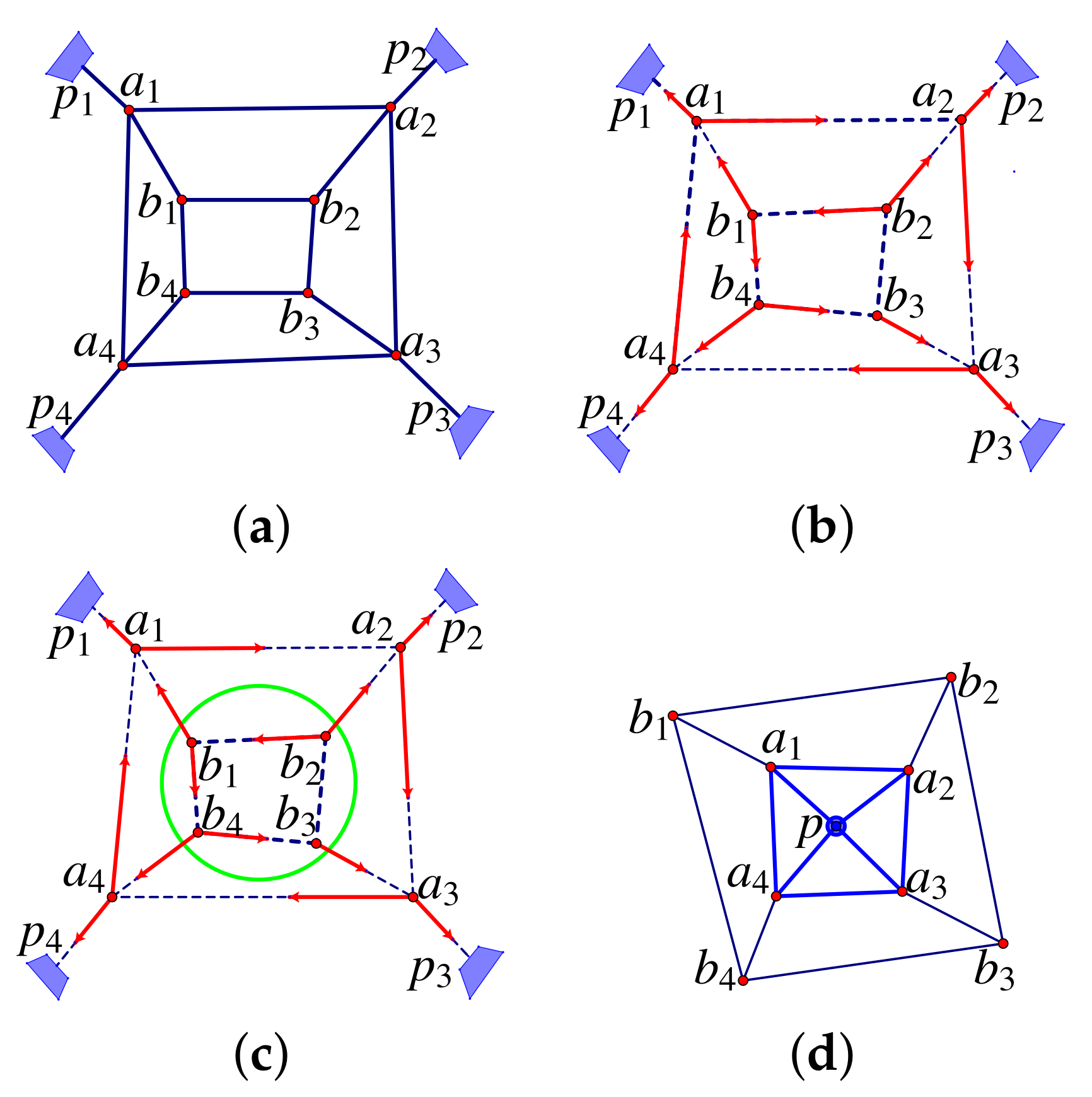
If the set P is contracted to a single vertex p, then the resulting contracted graph is a rigidity circuit.
3. 
Either the graph has a single inner vertex of degree 2 or each time we delete a vertex, the resulting pinned graph has a motion with non-zero velocity at all inner vertices (in generic position).
4. 
Deletion of any edge from G results in a pinned graph that has a motion with non-zero velocity at all inner vertices (in generic position).
5. 
Any 2-directed orientation of G is strongly connected.
Example 23.
Consider the pinned framework in Figure 33a. It has a 2-directed orientation (b) so it is pinned isostatic. The circle in (c) highlights a set of directed edges in one direction which disconnects the pinned graph into two components, so it is not strongly connected and therefore is not Assur. The subgraph outside the circle is Assur. If the four directed edges crossing the circle are pinned, the subgraph inside the circle, with these edges pinned, also forms an Assur graph. In general, identifying all the pins identifies a (sub)-circuit-a subgraph which, with pins identified becomes a circuit-as an Assur graph: in this case with vertices V = { a 1 , a 2 , a 3 , a 4 , p } .
Example 24.
Consider the example in Figure 34a. This is isostatic, as the 2-directed orientation in (b) confirms. As a 2-directed graph, the orientation is strongly connected. When the pins are all identified, there is a single circuit (c) which includes all vertices and all edges. There is a (non-generic) singular realisation (d), where there is a non-trivial infinitesimal motion fixing the pins, which is represented visually with a parallel drawing of all the inner vertices (red arrows). Parallel drawing is discussed in much more detail in our companion paper [27]. (c) and (d) are illustrations of Theorems 10 and 11.
Theorem 11
(Servatius, Shai, Whiteley [105]). A pinned graph G is an Assur graph in P 2 , if and only if it has a realisation p in P 2 such that
1. 
( G , p ) has a unique (up to scalar) equilibrium stress which is non-zero on all edges; and
2. 
( G , p ) has a unique (up to scalar) infinitesimal motion, and this is non-zero on all inner vertices.
These special positions p will be preserved by projective transformations.
Conjecture 2 
([105]). Let G be an Assur graph and let ( G , p ) be a framework in P 2 with a single equilibrium stress which is non-zero on all edges. Then there is a unique (up to scaling) non-trivial infinitesimal motion that is non-zero on at least one end of each bar.
The converse does not hold. If we pin a triangle with three bars to pinned vertices, it is Assur and the pinned pure condition has the triangle factor times the factor for the three pinning edges. If the triangle is collinear, then the stress is zero on some edges.

8. Polarity for Rigidity

Polarity is one of the basic transformations of classical projective geometry. When does this transformation generate a rigidity correspondence? The answer is that there are known correspondences in 2- and 3-dimensions. Polarity in the plane changes infinitesimal motions to liftings to 3-space [113], so we will defer that presentation to our companion paper [27]. We will will connect this plane correspondence into 3-dimensions (below) through coning. We are not aware of any strong rigidity results using polarity in dimensions 4 [113,114]. We are aware of the use of polarity in other metrics (e.g., the sphere in all dimensions) and even in recent work in multivariate splines [115].

8.1. Duality and Polarity for Projective Geometry

The primary example we will explore in this section is polarity in dimension 3. However the broader applications of polarity will include whole sections of our companion paper Projective Geometry of Scene Analysis, Parallel Drawing and Reciprocal Drawings [27], where parallel drawing and liftings in scene analysis are explicitly explored as combinatorial duals, and geometric polars, of one another, in all dimensions.
In plane projective geometry, there are axioms for points and lines, and they have an explicitly dual form: if you take theorems for points and lines, and swap the terms, replacing points by lines and lines by points, the entire theory is unchanged. For example, any two distinct points lie on a unique line, and any two distinct lines intersect in a unique point.
In a general dimension d, duality pairs subspaces of P d of projective dimension k and projective dimension d k 1 , reversing inclusions and preserving incidences. More generally, such a map is also called a correlation. The correlation is invertible, and if this correlation is its own inverse (that is, if it is an involution) then it is called a polarity. If we write the projective points as x = ( x 1 , x 2 , , x d , x d + 1 ) and the hyperplanes in dual coordinates as u = ( u 1 , u 2 , , u d , u d + 1 ) , then the incidence of the point x on the hyperplane u is given by the equation
x 1 u 1 + x 2 u 2 + + x d u d + x d + 1 u d + 1 = 0 .
In vector space terms this is sometimes named orthogonality but we prefer incidence, and the hyperplane can be identified with the space of points incident with the hyperplane.
There are two polarities which are central to our vision. One is the ‘natural’ polarity in which we do not change any of the coordinates, but just switch our interpretation of the coordinates of the points as the coordinates of hyperplanes, and vice versa. This correlation is an abstract involution but does not immediately have a geometric representation.
The second geometric construction (which can be visualized in P d ) is named polarity about a quadric [116]. This already appeared for biparite frameworks in Section 7.3. If we focus on the points which lie on their polar planes in the natural polarity, we see the equation x 1 2 + x 2 2 + + x d 2 + x d + 1 2 = 0 is a quadric surface in P d . For a given non-degenerate quadric surface in P d , there is a geometric construction of a polarity. This takes points on the quadric to the tangent hyperplane through the point. For the plane, we saw a brief introduction in Figure 23.
We also recall that going from a framework to the momenta of the vertices and centers of motions of the bars is also a duality, but is generally not a polarity, except for bipartite frameworks with vertices on a quadric (Proposition 1).
The origins of the name ‘polarity’ become visible when we consider the ‘natural’ polarity on the sphere and the elliptical model of projective geometry with antipodal points identified. This is also referred to as duality on the sphere. Every hyperplane on the sphere (e.g., the equator) has two antipodal poles. When the pairs of antipodal points are collapsed to form the elliptic model of the projective space, there is a complete pairing of hyperplanes and points, so there is a duality which is an involution—a polarity. This a geometric image of the natural polarity above. This polarity on the sphere takes a distance constraint (bar) between two points to an angle constraint between the two hyperplanes. We will return to this in Section 8.4.

8.2. Sheet Structures and Polarity for Rigidity in R 3

We next introduce hinged sheetworks with planes and edges as the polars of bar–joint frameworks, preserving rigidity when we interpret the planes as statically rigid frameworks on the incident edges. These were mentioned, independently, in the work of a Danish Architectural Engineer Ture Wester, and were also mentioned in passing in [97]. The one published study of hinged sheetworks uses static rigidity [113], showing how the forces applied to a face in its plane transmits through the statically rigid framework of a face (a) and how a force applied to an edge splits into two forces in the two distinct faces at the edge (b), Figure 35. The equilibrium condition for forces at the original vertex becomes an equilibrium condition for the forces applied in the plane of the face. We can transfer all of the definitions for static rigidity to the hinged sheetworks following [113].
There is a companion infinitesimal rigidity version of this theory using plane centers of motion for vertices polarizing to point centers of the sheets. It has yet to receive a proper published exposition, but the gist can be seen by polarizing the theory of momenta and centers of motion of bar and joint frameworks. If the polarity is Φ , then Φ ( a i ) = P i is the polar plane. The momentum of a vertex M ( a ) becomes a weighted point center Φ ( M ( a ) ) = M ( Φ ( a ) ) in the plane of the polar sheet. This point center of a sheet presents the component of the velocities of points in the sheet which lies within the plane of the plane-rigid sheet. The momentum of the hinge { i , j } is the polar center of the hinge Φ ( a i , a j ) , a weighted line segment in the line joining the centers of motion of the two sheets. The hinge condition is the polar of the bar condition in terms of projective momenta: [ M ( a i ) a j ] + [ M ( a j ) a i ] = 0 becomes [ Φ ( M ( a i ) ) Φ ( a j ) ] + [ Φ ( M ( a j ) ) Φ ( a i ) ] = 0 .
There is a fully projective version of all this theory of sheets, but it has so far only been published in vocabulary of R 3 [113].
Definition 1.
A hinged sheetwork ( G , P ) in R 3 is an ordered pair consisting of a graph G = ( V , E ) and an assignment of weighted plane sections P i to the vertices in projective 3-space such that P i P j 0 if i j E .
Definition 2.
Anequilibrium loadon a hinged sheetwork is an assignment of dual 2-extensors (forces), L = ( L 1 , , L | V | ) , to the sheets such that for each sheet we have L i P i = 0 and i = 1 | V | L i = 0 . Aresolution of the load L by a hinged sheetworkis an assignment of scalars λ i j to the edges i j E such that, for each sheet P i :
j : i j E λ i j P i P j + L i = 0 .
A hinged sheetwork isstatically rigidif every equilibrium load has a resolution. Astatic stressis a resolution of the zero load, i.e., a set of scalars λ i j for the edges such that L i P i = 0 at each sheet P i , sum over all edges attached to the sheet. A hinged sheetwork isindependentif the only static stress is the trivial stress with all scalars zero (otherwise it isdependent) and isisostaticif it is statically rigid and independent.
With a projective lens, it would be nice to have a good projective matrix for this. We propose that this should be the polar of the projective statics matrix for bar and joint frameworks.
Definition 3.
A hinged sheetwork ( G , P ) and a bar-and-joint framework ( G , p ) , both in R 3 , arepolarif there is a non-singular linear transformation T and a homogeneous multiplier H (a set of scalars h i , i V ) such that for each vertex i of G:
P i = h i T ( p i ) ( o r e q u i v a l e n t l y p i = T 1 ( P i ) / h i ) .
Theorem 12
([114]). A hinged sheetwork ( G , P ) and any polar bar-and-joint framework ( G , p ) in R 3 have the same static properties:
1. 
( G , P ) is statically rigid if and only if ( G , p ) is statically rigid;
2. 
( G , P ) is independent if and only if ( G , p ) is independent;
3. 
( G , P ) is isostatic if and only if ( G , p ) is isostatic;
4. 
the spaces of equilibrium loads are isomorphic;
5. 
the spaces of resolved loads are isomorphic;
6. 
the spaces of stresses are isomorphic.
Example 25.
Figure 36 illustrates the polarity with a statically rigid octahedral framework going to a statically rigid hinged sheetwork on a cube, where each face is some statically rigid framework in the plane of the face. Note that we are really selecting from an equivalence class of all statically rigid sub-frameworks on vertices in the face. The equivalence is a result of a general substitution principle which is highlighted in the substitution principles in the next subsection.
Recall from Example 11 that the pure condition for the octahedron is that four opposite faces meet in a point. Under polarity, this condition must become that the four opposite vertices of the sheetwork cube are coplanar. If one set of four opposite vertices is coplanar, then the other four vertices must also be coplanar.
Remark 4.
For complete bipartite frameworks in P 3 with vertices on a quadric, we have observed that the polarity Φ about this quadric generates (up to weights) the projective momenta and centers for a motion of the bar–joint framework (Section 7.3). This same polarity Φ also generates a sheetwork with sheets that are tangent to the quadric at the vertices of the framework. For simplicity, assume the quadric is the unit sphere. The sheetwork has a non-trivial infinitesimal motion, because the bipartite framework did, by Theorem 12. We claim that the vertices and edges of the original framework are (up to weights) the momenta for the motion of the sheetwork.
As noted in the introduction to this subsection, the polars of the momenta of the original framework are (up to weights) the projective centers of a non-trivial sheetwork. Since the sheetwork is also the polar of the bar–joint framework, the momenta of the sheetwork are, up to weights, the original bipartite framework. The vertices of the original framework are centers of motion for the sheets tangent at the vertices, and the edges of the bar–joint framework are momenta for the hinges (up to weights). Together these form a linked pair of structures around the quadric for which one gives the infinitesimal motions (momenta) of the other.
Remark 5.
There is a polarity for infinitesimal motions of plane frameworks [113] which can now be integrated into this discussion of sheetworks as polars of frameworks in P 3 , with proper attention to centers of motion, and momenta as we have been developing them. We sketch this new connection. We place a plane framework into the plane z = 1 in R 3 , with no vertex at the origin. We then take a cone to the point at infinity up the z axis and take the polar about a right circular cylinder. This gives a sheetwork in P 3 . The original vertices become vertical planes and the bars become the (vertical) intersection of the two sheets. The cone point becomes the plane at infinity as its sheet.
In the plane z = 0 , we have lines for the original joints and points for the original bars, as a cross-section of the polar sheetwork. In addition, the centers of motion of the sheets corresponding to the vertices lie on the lines in the plane z = 0 , and the centers of motion of the vertical lines pass through the intersections of these lines. The infinitesimal motions of the original plane framework now correspond to lifting or tilting the lines along the vertical planes, rotating about the point centers of plane sheets, which are now in the plane. This polarity is the essential construction of [113] and reappears in our companion paper [27].
There is a modification of sheetworks—the class of jointed-sheetworks—which is closed under polarity (Figure 37.)
Definition 4.
Ajointed-sheetworkis a bipartite incidence graph G = ( A , B ; I ) with an assignment P i of weighted plane segments (3-extensors) to the vertices in A and an assignment p j of weighted points in projective space (1-extensors) to the vertices in B such that P i p j = 0 (the point lies on the plane) for each pair ( i , j ) I .
Since these jointed-sheetworks include bar–joint frameworks, all the same gaps in combinatorial characterisations of independence and infinitesimal rigidity in R 3 remain.
Notice that the entire presentation here was thoroughly projective, so the theory must immediately include points, edges, and faces at infinity. It can also be presented with point centers of motion for sheets and plane momenta for joints. These have not yet been explored in appropriate detail.
With the same projective lens, there is an immediate transfer of infinitesimal and static rigidity of sheetworks to Minkowski space both via polarity in that space and also with a direct transfer of the rigidity analysis of each of the structures from Euclidean space. Similarly, the infinitesimal and static rigidity of sheetworks transfer sheets to bar–joint equivalence classes of sheets, in all projective metrics, including spherical frameworks.
In R 3 , polarity takes a pure condition on points for bar–joint frameworks to a polar pure condition on faces for sheet structures. Analogously, there will be a pure condition for point and sheet structures with variables for both points and faces in the polynomial. Note that polarity within spherical space (and hyperbolic space) takes distance constraints to angle constraints [69]. This is very different than polarity in the Euclidean space, followed by direct transfers. We return to this connection in Section 8.4 for a special class of frameworks: triangulated spheres.
Remark 6.
There are a number of avenues for further exploration of sheetworks. Some of these might be recognized in actual models, if we have sufficient vision. Figure 38 illustrates transformations among the various forms of sheetworks. We end with a few areas for further extensions.
1. 
There is a complete geometric theory of infinitesimal motions of sheetworks with projective centers of motion. Each sheet has a point centre in the sheet, and the two centres on sheets at a shared edge satisfy a compatibility condition which is the polar of the condition for bar–joint frameworks. Does this offer additional insights?
2. 
What happens with points, lines and sheets at infinity?
3. 
What about four copunctual sheets—the polar of four coplanar points of a tetrahedron. The polar will be four sheets through a single point, but with six specified hinge lines through this point. What will the infinitesimal motions look like?
4. 
Are there any examples of sheetworks with finite motions where sheets remain as coplanar sheets? Even the polar of the double banana—with two sheets joining two bodies—only has finite motions which warp these joining sheets. For example, the polar of the double banana shown in Figure 39b,c only has infinitesimal motions which bend the two sheets (d), though as a triangulated model it does have a finite motion.
5. 
Consider the polar of K 4 , 6 with the four points coplanar. The four points become four sheets which are co-punctual, with no hinges (edges) among them. As the polar of 6-valent vertices, these four sheets are hexagonal sheets. These sheets must meet in 6 four-valent sheets. This type of geometry has yet to be explored.
6. 
The analogue of tensegrity frameworks are slotted sheetworks. (We will formally introduce tensegrities in Section 12).

8.3. Substitution Principles

The fact that all isostatic frameworks on the vertices of a face are equivalent illustrates a general substitution principle for subframeworks in a subspace [97]. These substitution principles apply within all projectively based metrics. They are basically about equivalent bases within subspaces of the rows of a matrix.
Theorem 13
([97]). Suppose a framework in P d has no non-trivial equilibrium stress and has a subframework among k joints that is statically rigid in the affine space spanned by the joints. Moreover suppose that a modified framework is created by replacing this subframework by a new isostatic subframework on these k joints. Then the entire modified framework has no non-trivial equilibrium stress.
The idea (and proof) is simply that the rows of the isostatic subframework are the basis for a subspace and any such basis can be replaced by another basis that resolves the same loads (Figure 40). These substitutions generate equivalence classes of frameworks, as was found for hinged sheetworks and jointed sheetworks. The substitution principles also arise naturally in Alexandrov’s Theorem in the next subsection.
These substitution principles extend immediately to all the projective metrics. The principles also include points at infinity, if the matrices and rows include such points and edges. Similar substitutions should extend to the broader classes of geometric matroids (and matrices) which are found in Part 2 of this article.

8.4. Cauchy, Alexandrov and Polarity

There is a cluster of rigidity theorems which were initially proven for convex triangulated spheres in R 3 [117,118], but have generalisations to a broader class of structures in P 3 . There are higher dimensional extensions [97] with the 2-dimensional faces of a convex polytope in P d triangulated in their planes giving infinitesimal rigidity for the entire convex polytope P d [119]. The combinatorial analogue of Cauchy’s Theorem, which says that all triangulated spheres are generically rigid (proven by vertex splitting from a triangle [120]), transfers directly to bivariate splines on triangulated spheres (see Section 11 and [121]).
Definition 5.
A strictly convex polyhedral frameworkis a framework formed by
1. 
placing a joint at each vertex of a strictly convex polyhedron,
2. 
placing a bar along each edge of the polyhedron.
We note that the graph G = ( V , E ) of any triangulation of the sphere, by Euler’s formula, satisfies | E | = 3 | V | 6 . Thus, such frameworks are isostatic in P 3 if and only if there is no non-zero equilibrium stress. The proofs in [97,118] show there is only the all zero equilibrium stress.
Cauchy’s original proof was for a related theorem about the global uniqueness of convex triangulated polyhedra, within the class of all convex triangulated polyhedra. We give an infinitesimal rigidity version for an extended class of polyhedra which is found in the book of Alexandrov [122] and was reworked with statics in [97].
Theorem 14
(Alexandrov [97,122]). A strictly convex polyhedral framework in P 3 with joints at the vertices and bars on the natural edges, and additional bars to triangulate each face polygon which is not already a triangle, is isostatic (Figure 41).
Alexandrov further extended this geometric result by adding additional vertices along the original convex edges of the polyhedron, and ensuring that these vertices are included in isostatic frameworks in both of the faces at this edge [97,122]. This preserves infinitesimal rigidity in P 3 .
Note that the geometric polar of a triangulated spherical polyhedron (or simplicial polyhedron in P 3 ) is a hinged sheetwork on a simple polyhedron, which fits within Alexandrov’s Theorem.
As theorems about the infinitesimal rigidity of bar–joint frameworks, the results of Cauchy and Alexandrov transfer directly to spherical, hyperbolic, Minkowski and de Sitter spaces. They also extend to include vertices and edges at infinity. Some variants of Cauchy’s Theorem include sending a vertex to infinity, creating an open polyhedron with edges fanning out to infinity.
We can extend these theorems to convex simplicial polytopes in higher dimensions. The proof connects the 3-dimensional result to the vertex figure viewed as a cone of a convex polytope of the next lower dimension [97]. It is also related to Alexandrov’s theorem in the sense that within their 3-space, the cells of a 4-polytope are statically rigid frameworks, once all 2-faces are triangulated.
Definition 6.
A strictly convex 4-polytopial frameworkis a bar–joint framework in P 4 built on a strictly convex 4-polytope by
1. 
placing a joint at each vertex of the polytope,
2. 
placing a bar on each edge of the 4-polytope.
We can give the 4-space analogue of Theorem 14.
Theorem 15
(Whiteley [97]). A strictly convex 4-polytopial framework, with all 2-faces triangulated, is infinitesimally rigid in P 4 .
Clearly it follows that the graph G = ( V , E ) of the convex 4-polytope satisfies | E | 4 | V | 10 . As Kalai observed [119], this proves a case of the lower bound theorem for 4-polytopes. This infinitesimal rigidity of polytopes with 2-faces triangulated (or made infinitesimally rigid in their plane) has been extended to arbitrary dimensions, giving | E | d | V | d + 1 2 for a convex simplicial d-polytope [97,119]. It would be valuable to describe the rigidity of various forms of sheet structures in higher dimensions. In our companion paper [27], we will explore the 2-dimensional analogue where collinear vertices are spanned by a tree of edges; a “tree-line”.
There is a different polarity in hyperbolic and spherical geometry which does not connect to sheet structures. However, the infinitesimal rigidity of sheet structures, as implicitly bar–joint frameworks, does transfer to spherical space and hyperbolic space. The polarity in the spherical and hyperbolic metrics takes distance constraints to angle constraints [69]. This adds another rich layer to possible explorations, bringing in angles which are not captured within the Euclidean space. We will include some additional partial results on angles in Euclidean space when we look at Minkowski decomposition in our companion paper [27].
Remark 7.
There is a separate, but related, study of static and infinitesimal rigidity of appropriately smooth surfaces, perhaps with some singularities [123]. These were recognized, at least implicitly, as projectively invariant properties and there has been some transfer of methods, results, and questions between the fields [65,124]. It is worth also pointing out a key difference for smooth surfaces. Static rigidity and infinitesimal rigidity are not equivalent for smooth surfaces: the equivalence for finite frameworks made an essential use of row rank = column rank for finite dimension matrices, but for smooth surfaces the concepts correspond to the row and column dependencies of infinite-dimensional matrices. This was already evident when static rigidity did not imply infinitesimal rigidity for discrete infinite frameworks (Remark 1). There are further results and conjectures on projective transformations, polarity, etc. in the smooth setting.
Applsci 11 11946 i002

9. Body-Bar Frameworks

By expanding vertices to be larger rigid structures or rigid bodies, we find the combinatorics of generic rigidity simplifies, and we can give full combinatorial characterisations in all dimensions with efficient algorithms and with informative projective geometric conditions for singularity [58,125]. This setting has been a playground for developing results which we can then work to extend back to bar–joint frameworks. The theory has also been the basis for conjectures and then theorems about the rigidity of molecular structures, particularly proteins [126] (Section 10.5). The full theory is projectively invariant and will be presented with projective coordinates. This projective presentation is the only efficient way to work with the algebraic representations for these structures.
Take a loopless multigraph G = ( V , E ) where V = { 1 , 2 , , | V | } . We define a body-bar framework ( G , p ) in P d , with each edge a b represented by the weighted 2-extensor p a p b = a b = a b (with a < b ) and its Plücker coordinates in P d .
Definition 7.
The rigidity matrix M ( G , p ) for the body-bar framework ( G , p ) in P d has one row for each bar and d + 1 2 columns for each body, with the columns for B 1 followed by those for B 2 , etc. If ( a , b ) is a bar with endpoints a in body B i and b in body B j , then the row corresponding to ( a , b ) in M ( G , p ) has the 2-extensor a b in the d + 1 2 columns for B i and b a = a b in the d + 1 2 columns for B j , and 0 in all other columns. (Under this definition, many frameworks are equivalent. Indeed, all that matters is the 2-extensor, or line, a b , not the location of the two points a and b on that line, as long as they are distinct.) Amotionof ( G , p ) is an assignment of a center Z i to each body B i , 1 i m , so that the length of each bar ( a , b ) is instantaneously preserved, that is, Z i * · a b Z j * · a b = 0 . (Recall the definition of dual extensors in Section 3.1). If we let Z * be the vector ( Z 1 * , Z 2 * , , Z m * ) of length m d + 1 2 then we require that M ( G , p ) ( Z * ) T = 0 .
Anequilibrium stressof a body-bar framework ( G , p ) in P d is a row dependence of M ( G , p ) . A body-bar framework ( G , p ) in P d isindependentif the only equilibrium stress is zero on all edges. A body-bar framework ( G , p ) in P d isinfinitesimally rigidif M ( G , p ) has rank d + 1 2 ( | V | 1 ) .
As noted above, there are many equivalent body-bar frameworks with the bars sharing the same extensors, but perhaps using different points along the same lines. Multiplying the bar-extensors by a scalar can correspond to sliding a pair of points along the line, at a different distance or just to a different weighting of the projective points. Furthermore, the bodies do not have any location. Any point can be assumed to lie on body B i , and the same point can be assigned to lie on another body along another line. When looking at an application, or a coming figure (e.g., Figure 42 and Figure 45) we will depict a set of locations for the ends of the bars, but the analysis will apply to equivalent body-bar frameworks. This equivalence is also projective, so the end of a bar, or an entire bar, can ‘lie at infinity’ in a figure or an application of the results.
Theorem 16
(Tay [58,125]). For a generic set of lines p and a body-bar framework ( G , p ) in P d , the following are equivalent:
1. 
( G , p ) is infinitesimally rigid and independent as a body-bar framework;
2. 
| E | = d + 1 2 ( | V | 1 ) and for all non-empty subsets of edges E on bodies V , we have | E | d + 1 2 ( | V | 1 ) ;
3. 
G can be partitioned into d + 1 2 edge-disjoint spanning trees.
The projective motions of all of P d are obtained by setting all Z * (see Definition 7) equal to a given screw. These are always motions of ( G , p ) . Since these motions form a subspace of dimension d + 1 2 , the maximum rank of M ( G , p ) is ( m 1 ) d + 1 2 . We say ( G , p ) is isostatic if M ( G , p ) has rank ( m 1 ) d + 1 2 and the rows are linearly independent.
There is a connectivity condition for body-bar frameworks which is sufficient for infinitesimal rigidity in all dimensions.
Corollary 6
([49]). If a multigraph is d ( d + 1 ) -edge-connected, then almost all body-bar frameworks on this graph in P d are infinitesimally rigid.
We note that this connectivity is the minimum possible in general, as there are ( d ( d + 1 ) 1 ) -edge-connected graphs which are generically flexible. These examples extend the example in [38] for d = 2 . For bar–joint frameworks, 6-connectivity in the plane is sufficient for rigidity by results of Lovasz and Yemini [38], who also showed that 5-connectivity is not sufficient. It is a conjecture that d ( d + 1 ) -connectivity is also sufficient for generic rigidity of bar–joint frameworks in d-space. Moreover, the recent results of Clinch, Jackson and Tanigawa [25] show that, when d = 3 , 12-connectivity is sufficient (whereas 11-connected is not sufficient) for rigidity in the maximal 3-dimensional abstract rigidity matroid. However there is currently no known k such that k-connectivity implies rigidity for bar–joint frameworks when d > 2 .

9.1. Body-Bar Combinatorics

We offer more insight into the tree characterisation in Tay’s Theorem, following the analysis in [58]. This is adapted using more recent approaches based on Laplace decompositions, such as [106]. The second key ingredient is finding a special configuration that is easily analyzed and is still infinitesimally rigid—in this case placing trees along edges of a simplex. If we take the basic body-bar rigidity matrix, we can square it up by deleting the columns corresponding to the last vertex (body), with no change in the rank but a reduction in the kernel. A single body has exactly the trivial motions of the framework, so this squaring-up is the same as a tie-down of this one body, so all trivial motions are removed by this deletion without any loss of rank.
Example 26.
Consider a body-bar framework on the line. On a line, a point has the full space of trivial motions of a body—which has dimension 1. A framework is infinitesimally rigid if it is connected, or equivalently contains a spanning tree (Figure 43).
These trees are recorded in the body-bar rigidity matrix on the line as
B 1 B 2 B 3 B 4 B 5 ( 1 , 2 ) ( 1 , 3 ) ( 3 , 4 ) ( 3 , 5 ) ( 1 1 0 0 0 1 0 1 0 0 0 0 1 1 0 0 0 1 0 1 ) B 1 B 2 B 3 B 4 B 5 ( 1 , 2 ) ( 2 , 3 ) ( 3 , 4 ) ( 4 , 5 ) ( 1 1 0 0 0 0 1 1 0 0 0 0 1 1 0 0 0 0 1 1 ) .
Notice that if we delete the last column for B 5 , the square matrix has a non-zero determinant.
This is a model for larger d, just repeated d + 1 2 times. If we then reorder the remaining d + 1 2 ( | V | 1 ) columns by first taking the first coordinates B j 1 for j = 1 , m 1 , then the second coordinates B j 2 for j = 1 , , m 1 , and so on until finally taking the last coordinates B j d + 1 2 for j = 1 , , m 1 , then the determinant of the resulting square matrix can be calculated by a block Laplace expansion using blocks for each of the m 1 columns. The determinant is non-zero only if there is a non-zero term in this expansion | L 1 | | L 2 | | L d + 1 2 | 0 . These blocks for this non-zero term generate a decomposition of the edges of the body-bar framework into d + 1 2 blocks which we write as ( A 1 1 , A 1 2 , , A m 1 1 ) , , ( A 1 d + 1 2 , A 2 d + 1 2 , , A d + 1 2 m 1 ) , giving the matrix: Applsci 11 11946 i009 The determinant of any one of these diagonal blocks, which has rows which are multiples of rows of the graphic matroid on the edges is non-zero if and only if the edges form a spanning tree on the bodies [49,58,127]. Thus, these terms generate the desired decompositionof the edges into ( d + 1 2 ) spanning trees, partitioning the ( d + 1 2 )(m − 1) edges.
Conversely, if we have d + 1 2 trees T 1 , T 2 , T d + 1 2 partitioning the edges, then we can create an isostatic body-bar framework by assigning each tree to a distinct extensor for the edges of a projective simplex:
( 1 , 0 , , 0 ) ; ( 0 , 1 , , 0 ) ; ; ( 0 , 0 , , 1 ) .
This creates the following matrix: Applsci 11 11946 i010
In this matrix, each [ T i ] is the signed incidence matrix of the tree T i [58,127]. From basic work on the cycle matroid (the matrix for rigidity on the line), this has a non-zero determinant. Thus, for this position, which uses the lines of the edges of a K d + 1 2 , we have an isostatic body-bar framework.
Figure 44 illustrates this for d = 2 (a) and d = 3 (b) using the edges of a simplex in projective space, with vertices at the origin and at infinity to simplify the Plücker coordinates. With this image of the trees along the edges of a simplex, we see that it is possible to specialise the geometry of the edges of independent body-bar frameworks and maintain independence.
For example, in 3-dimensions, if two bodies share edges in trees T 1 , T 2 , T 3 , these bars can be made concurrent in a point ( 0 , 0 , 0 , 1 ) in the larger framework forming a pin, maintaining the independence. Which patterns of pins can a body-bar framework sustain? We note that two bodies cannot share two pins, as that would become a redundant ‘hinge’. Alternatively, the 3 bars connecting the same two bodies could share the other three trees T 4 , T 5 , T 6 , which are coplanar, so they form a ‘sheet’ connection between the bodies. Two bodies could have both types of shared connections. We are not aware of a complete analysis of which pin and sheet connections can occur in an isostatic body-bar framework.
It is a standard goal in the combinatorics of rigid structures to offer a recursive construction of all isotatic structures from a simple base case. For body-bar frameworks this type of inductive construction is available, starting from a single body. This is implicitly described in [128], where the larger goal was to capture all minimally redundant body-bar frameworks. These inductions also build on the prior work of Tay and Whiteley [37,125,129,130].

9.2. Body-Bar Projective Conditions and Centers of Motion

White and Whiteley [58] present an analysis of the pure conditions for body-bar frameworks in P d with techniques of directed graphs analogous to those described in Section 7.6. In that paper, there was a focus on how the conditions relate to infinitesimal motions of bodies when an edge is deleted from a generically isostatic body-bar framework or becomes dependent due to a special projective configuration.
Figure 45 illustrates a few simple special (singular) positions for body-bar frameworks in the plane [58]. More generally, White [52,57] explores a number of applied geometric results which can be well described in the projective Grassmann–Cayley algebra.
Example 27.
Figure 45a shows a generic rigid body-bar framework in the plane with two bodies connected by 3 independent bars. The row of the rigidity matrix for a bar a b imposes the condition: a b S 1 a b S 2 = a b ( S 1 S 2 ) = a b ( S 12 ) = 0 , where S 1 and S 2 are the centers of motion for the bodies B 1 and B 2 , and S 12 is the relative center of motion of the bodies. Projectively, this says that the relative center must lie on the line a b . This also holds for the bars c d and e f . There is a non-trivial infinitesimal motion if and only if there is a projective point on all three bars (b). Given such a point, we can choose an arbitrary center S 1 and find a center S 2 which produces this relative center (c). If the three bars meet in a point S 12 , projectively (including all bars being parallel), then there is a non-trivial infinitesimal motion, and vice versa. One vision of this is: holding body B 1 fixed, body B 2 can rotate about the point S 12 which lies on all the bars.
Example 28.
Consider the plane body-bar framework in Figure 46a. The pure condition for this example has a projective construction as follows: writing C ( G ) = ( a b ) ( c d ) ( e f ) , we see that C ( G ) = 0 precisely when the three points of intersection determined by the pairs of bars are collinear. In general, when we consider the relative centers of any three bodies in the plane with a non-trivial infinitesimal motion, we obtain:
S 12 + S 23 + S 31 = [ S 1 S 2 ] + [ S 2 S 3 ] + [ S 3 S 1 ] = 0
which is a simple accordion collapse where reordering the brackets gives middle terms ( S i + S i ) = 0 . Since [ S i S j ] is a projective point (with a weight) for the relative centre of the two bodies, this equation says that the three relative centres must projectively add to 0. Projectively, three points can only add to 0 if they are collinear.
This result also illustrates a more general theorem of Arnhold–Kempe [52,57]: If three bodies are in motion in the plane, the relative centers of motion of the three pairs of bodies are collinear in the projective plane. Notice that this is a projective statement. Some, or even all, of the relative centers can be on the projective line at infinity corresponding to relative translations. If the bars in Figure 46a are parallel, then this is what happens to the relative centers.
The body-bar matrices have several simplifying features compared to the bar–joint matrices. The columns of any single body effectively provide a handy tie-down. A further simplifying feature of the body-bar matrices is that an entry a i b j occurs in just one row (recall Definition 7), and the determinant of a matrix after a tie-down is linear in the Plücker coordinates of each bar.
The entire analysis of factoring for these pure conditions simplifies to finding the subgraphs which are themselves generically isostatic in P d [58]. Moreover, setting an irreducible factor = 0 , and taking a generic configuration within this algebraic variety only creates a single equilibrium stress and a single non-trivial infinitesimal motion, which is non-trivial on all pairs of bodies with edges in this factor. These body-bar frameworks appear to behave exactly the way we wished Assur graphs would in higher dimensions. Figure 47 illustrates the decomposition of a body-bar framework, taken from [58].
Example 29.
Consider the example in Figure 47a as a body-bar framework in the plane. Whether pairs of bars between two bodies meet in a shared point is not relevant, except to focus our vision. There are two underlying minimal isostatic components which are boxed in part (b) of the figure. Each of these will have a pure condition on just its bars. Then the two components can be joined to form a larger isostatic body-bar framework. If we effectively contract the two minimal frameworks to form a single body, the remaining edges have an additional pure condition (actually one for joining two bodies with three bars, which we saw above). Overall, each edge lies in exactly one condition, and the overall pure condition will be the product of these three factors.
While making these connections, we observe that it could be timely to expand the full range of investigations in [58] with the added perspective of recent results and techniques from Assur graphs (Section 7.7). In particular, we conjecture that if a subgraph which is generically isostatic has a realisation with exactly one non-zero stress on all edges, and a single non-trivial motion between all pairs of bodies, then the subgraph has an irreducible pure condition.
We note that polarity in P 3 takes 2-extensors to 2-extensors. Overall, polarity in P 3 takes bodies to bodies (dual bodies) and 2-extensor bars to 2-extensor bars. Therefore, polarity will preserve the infinitesimal rigidity of body-bar frameworks. So the configurations that make a pure condition equal to zero will be closed under polarity in P 3 .

9.3. Projective Line Dependences and the Stewart Platform

Consider two bodies in d-space joined by d + 1 2 bars. This is infinitesimally rigid if and only if these lines are independent in projective space. The Stewart Platform (Figure 48) illustrates how the line geometry in P 3 appears in the analysis of relative motions of two bodies [6,131,132]. In particular, the Stewart Platform with a zigzag pattern of shared vertices [133], as shown in Figure 48b, has independent connecting bars and is hence generically isostatic. This is also called a hexapod.
A classic textbook [134], written for North American structural engineering students, chose to simplify the communication of dependencies for 6 bars connecting a body to the ground by only illustrating the singular configuration where all bars meet a single line (Figure 48c—with line a b ). This choice was because the more careful complete communication would have required more knowledge of projective geometry, which the author knew but the engineering students did not. This lack of knowledge of projective geometry may still hold true, at least in North America. This singular configuration with all braces meeting a single line was at the heart of the Tay River Bridge disaster, also illustrated in [102].
Consider the 6 × 6 matrix formed by the coordinates of 6 lines joining two bodies in P 3 :
41 42 43 23 31 12 a 1 b 1 a 2 b 2 a 3 b 3 a 4 b 4 a 5 b 5 a 6 b 6 ( ( a 1 b 1 ) 41 ( a 1 b 1 ) 42 ( a 1 b 1 ) 43 ( a 1 b 1 ) 23 ( a 1 b 1 ) 31 ( a 1 b 1 ) 12 ( a 2 b 2 ) 41 ( a 2 b 2 ) 42 ( a 2 b 2 ) 43 ( a 2 b 2 ) 23 ( a 2 b 2 ) 31 ( a 2 b 2 ) 12 ( a 3 b 3 ) 14 ( a 3 b 3 ) 24 ( a 3 b 3 ) 34 ( a 3 b 3 ) 23 ( a 3 b 3 ) 23 ( a 3 b 3 ) 13 ( a 4 b 4 ) 14 ( a 4 b 4 ) 24 ( a 4 b 4 ) 34 ( a 4 b 4 ) 23 ( a 4 b 4 ) 23 ( a 4 b 4 ) 13 ( a 5 b 5 ) 14 ( a 5 b 5 ) 24 ( a 5 b 5 ) 34 ( a 5 b 5 ) 23 ( a 5 b 5 ) 23 ( a 5 b 5 ) 13 ( a 6 b 6 ) 14 ( a 6 b 6 ) 24 ( a 6 b 6 ) 34 ( a 6 b 6 ) 23 ( a 6 b 6 ) 23 ( a 6 b 6 ) 13 ) S 41 S 42 S 43 S 23 S 31 S 12 = 0 0 0 0 0 0 .
Any non-zero solution to this matrix equation will be the six coordinates of a screw, which is a relative screw center for a motion of one of the bodies while the other body is fixed. In the language of the Theory of Screws [6,59,131], the bars are null lines of the screw. The null lines of a screw form a line complex which includes a pencil of lines through every point in space. If the screw solution is itself a line, then all the bars of the line complex intersect this line, forming a singular line complex, with the pencil of lines formed by joining some point to this line.
More generally, some configurations of lines are linearly dependent and therefore will support stresses. Others are independent in the sense that no linear combination will be dependent. The sums of such lines will create screws, but only some independent lines will generate additional lines as sums of the generators, rather than screws. We offer a brief illustration of the larger theory, nicely presented in [131].
Example 30.
We offer a short summary when independent lines generate other lines as linear combinations. 6 independent lines will generate all lines, and all 2-extensors (screws) as linear combinations.
When working with examples of frameworks, it is valuable to be able to detect the projective geometric dependence of bars. This is well presented in [131,132]. We will summarize some key observations about how dependencies of lines appear in 3-space. We begin with two lines and work up to six lines (Figure 49).
Two independent lines.
If two lines in 3-space are skew (not intersecting) then no other line will appear among the linear combinations. If two lines intersect, then all lines through this intersection in their plane will appear as linear combinations forming a projective pencil. This is projective, so if the lines are parallel meeting at infinity, then other coplanar and parallel lines lie in the same projective pencil.
Three independent lines.
If three lines are mutually skew, then they will lie on a ruling of a quadratic surface. Linear combinations will be other lines on the regulus of this quadratic surface. Four lines on this regulus will be dependent. This is something engineers have been trained to watch for, at least visually.
If three lines lie together in a plane, but are not mutually concurrent, then all other lines in the plane will be a linear combination of these three lines, As a dual, if three lines are concurrent, but not coplanar, they are independent and a fourth line through this point is dependent (Figure 49b,c). Figure 49c also shows four dependent lines since the two lines at A generate a plane pencil which includes the line AB, as does the plane pencil at B. With this common line AB, the four lines are dependent.
Four independent lines—line congruences.
Consider the lines in Figure 49c. The added plane at point C has lines which cannot be combinations of lines in the previous planes in Figure 49c.
A symmetric pattern for four independent lines is through (A,B,C) plus one line in each of the planes. The linear combinations of lines in a general line congruence will generate a single line through each point in space [131]. Another way to generate a line congruence is to take three lines generating all lines in a plane plus one line transversal to the plane. Dually, we could have three lines through a point plus one line not through the point. Again, each of these generates one line through each point in space, with additional lines for the special points in the generating plane.
Five independent lines—line complexes.
If we take one line, and all lines intersecting it, we find thesingular line complexwhich has one plane pencil through every point (finite or infinite) in 3-space (Figure 49d). There are more general line complexes. If we take a screw S, then the set of other screws S * which satisfy the equation S * S = 0 are the null lines of a screw mentioned above. As a single linear equation in the 6-space of screws, the solution space has dimension 5. Classical geometry [131,132] shows that this space is generated by sets of 5 lines, and for any point in space there is a pencil of lines. Dually, in any plane, there will be a pencil of lines.
Six independent lines.
Will generate all lines as linear combinations. Figure 48a,b gives some examples of 6 lines which are independent, at least generically.
In [58], the calculations with pure conditions for body-bar frameworks were used to calculate relative centers of motion when an edge was deleted or changed in length. There is more to be explored here within the projective lens.
Example 31.
Figure 50a gives another sample of 6 independent lines, for generic lines within the visible projective geometric conditions of three lines through point p and three lines in a distinct plane P. In (b) the dark blue lines are independent (subsets of (a)), while the red line l is in the spatial pencil of lines through p – a linear combination of the dark lines. In (c) the dark lines are again independent – generating all lines in the plane (redl) as linear combinations. in (d) the point p is placed into the plane P, so the shared line l (or any line in this plane pencil) is a linear combination of both the lines through p and the lines in plane P – the six lines are dependent by their projective geometry. Thus this configuration always is dependent with these projective conditions and there is a maximum of 5 independent lines
The polar of the configuration in (a) is an equivalent configuration to (a). The polar of (b) is a configuration equivalent to (c) and the polar of (d) is again equivalent to (d). In general, the independence of bars in body-bar frameworks is invariant under polarities which take the bars to new lines.
There is a rich vein of projective geometry and projective insights in the design and analysis for body-bar frameworks [59,132]. Viewing the design choices and analysis through a projective lens is an essential point of view.

9.4. Static Rigidity and Stresses in Body-Bar Frameworks

We can transfer the entire theory of statics to body-bar frameworks. One approach is to replace bodies by rigid bar–joint sub-frameworks. Instead, we will directly transfer the definitions, with illustrations from dimensions 2 and 3. Recall that forces are expressed with 2-extensors, which are also used for rows of the body-bar rigidity matrix.
Informally, the rows of the body-bar rigidity matrix share an important property: the equilibrium property says the sum of the entries within a single row, including all the 0 entries, is a b + b a + 0 = 0 . This property extends to all linear combinations of the rows, so an assignment of a wrench (sum of 2-extensors; recall Section 3.2) to all the bodies can only be in the row space if it satisfies the equilibrium property.
Definition 8.
Given a body-bar framework ( G , p ) in P d , aloadon ( G , p ) is an assignment W of a wrench (sum of 2-extensors) to each body. Anequilibrium loadon a body-bar framework is a load W such that i V W i = 0 . The linear combinations in the row space of the matrix satisfy the equilibrium condition. A resolution of an equilibrium load is an assignment of a scalar ρ e to each edge e and its row R e , such that e ρ e R e = W .
Example 32.
Consider the body-bar framework in Figure 51 with an equilibrium load (a). In (b) we graphically confirm this is an equilibirium load since the lines of three forces meet in a point and the free vectors add to 0. In (c) we recognize that the two bars joining to bodies generate a fan of possible lines for a resolution, going through the point of intersection, and three of those lines can be used to resolve the load. In (d) we give the resolving responses in the three lines which fully resolve the equilibrium load on the statically rigid body-bar framework in the plane.
In line with the theory for most types of finite structures with a rigidity matrix, infinitesimal rigidity requires that the column rank is d + 1 2 ( | V | 1 ) and static rigidity requires that the row rank is also d + 1 2 ( | V | 1 ) . This immediately gives the following result.
Proposition 8.
A body-bar framework in P d is infinitesimally rigid if and only if it is statically rigid in P d .
Example 33.
Consider the bicycle wheel in 3-dimensions (Figure 52). This can be represented as a body-bar framework with two bodies and the spokes as bars. However, the material of the thin spokes will only support forces in tension. For infinitesimal rigidity, we need aproper equilibrium stresswhich is positive on the spokes. With this sign restriction it is a tensegrity framework (Section 12). For example, we may only need 7 spokes which span the space of bars to make the wheel rigid – which can be enough bars to sustain an equilibrium stress ω between two bodies. If ω is a positive equilibrium stress on the 7 bars, then any load on the wheel and axle can be resolved on 6 independent bars. Adding a sufficiently large multiple of the positive equilibrium stress ω on the 7 bars, the load is now resolved on the spokes, with all coefficients positive. This gives a flavour of what we will explore further in Section 12.
This rigidity is not quite projective but it is locally projective: any small projective transformation will preserve the signs of the equilibrium stress and keep the body-bar framework statically rigid with a positive equilibrium stress on the 7 bars. We note that this approach requires only one bar beyond the minimal 6 for static rigidity—not the 12 tensegrity members that Buckminster Fuller speculated.
A cut set  S E of a body-bar framework is a subset E of edges whose removal separates the graph of the framework into two or more distinct components. The following theorem is folklore among civil engineers and gives a useful property of such cut sets [29].
Proposition 9
(Cut Set Equilibrium). Let S = { ( p i , q i ) : 1 i k } S be the edges of a cut set S of a framework ( G , p ) which are directed into a connected component of G S . Then for any equilibrium stress ω on the framework, i = 1 k ω i ( p i q i ) = 0 , where ω i ω .
For insight, consider a single body as the component. This property is immediate for a single body from the equilibrium condition. For an inductive proof, one then moves out to adjacent bodies and adds the individual equilibrium conditions and observes that cancellation occurs on any edges that now lie inside the larger component, leaving the correct equilibrium on the wider cut set for the expanded component. This cut set equilibrium condition is used by engineers to test whether a minimal framework, by count, is statically rigid. The proposition also holds in the more general context of bar–joint frameworks in P d .

9.5. Coning Body-Bar Frameworks

We are not quite ready to present a full analysis which mixes bodies and bars and takes a one-point cone, which would require an analysis of a combined body, bar, and single point framework. Such a geometric vision is behind why the results on body-bar frameworks will transfer to the spherical metric, and why coning may be interesting.
Imagine that we have a body-bar framework ( G , p ) in P d and a new point O P d + 1 . If we initially envision or ‘place’ O in body v 1 and add d + 1 bars from this point to each of the other bodies, then in an underlying bar-and-joint model of the body-bar framework, we have a cone framework in P d + 1 and infinitesimal rigidity is preserved. This gives one interpretation of the body-bar framework transferred to the spherical metric.
If we split the point O P d + 1 into a set of new vertices, one for every bar, this will retain the infinitesimal rigidity with all bars distinct and no lines of bars are assumed to meet. More directly, the added bars can be partitioned into d + 1 additional spanning trees. Any trees will work and we can have any duplication we wish. For example, we may choose the trees so that each of them forms a fan from the body v 1 , giving a total of d + 1 2 + ( d + 1 ) = d + 2 2 spanning trees. By Tay’s Theorem 16, this is sufficient for infinitesimal rigidity in P d + 1 (see Figure 53).
What about the converse? If we have a generically isostatic body-bar graph in P d + 1 , with d + 2 2 -spanning trees, removing any d + 1 spanning trees leaves d + 1 2 spanning trees. Therefore, for any choice of the deleted trees, we have a generically isostatic body-bar graph in P d by Theorem 16.
Remark 8.
As noted before, it does not matter which two distinct points along the line of a bar are designated as the endpoints at the respective bodies, as long as they are distinct. In particular, we could select a hyperplane for each body, and choose the endpoints of bars to the body to lie at the intersection of the line of the bar and the body’s hyperplane, at least generically. Things change when we go down one more dimension and place the bodies in a projective space of co-dimension 2. That is explored in the next section.

9.6. Rod and Bar Frameworks in 3-Dimensions

Tay [125,129] and Tanigawa [135] studied further interesting variants of body-bar frameworks, in which projectively smaller bodies, such as rods or collinear rigid bodies in P 3 , are linked with bars. They are worth describing, briefly, because they occur in applications and they have good combinatorial characterisations. In Section 10.7, we will return to rod and pin frameworks in the plane. Rods in P 3 start with 5 degrees of freedom, as a rotation of a rod about its axis is trivial. This suggests that the constraint count for a multigraph G = ( R , E ) of rods R and bars E joining pairs of rods will be | E | 5 | R | 6 .
Example 34.
Consider the simple rod and bar frameworks in Figure 54. With 2 rods joined by three bars, the count is | E | = 3 < 5 × 2 6 = 4 . Even clamped together one rod rotates about this pin (see the light line in Figure 54a). When we add a 4th bar, we can use the four bars to complete a tetrahedron, as in Figure 54b. This realisation generalises to other realisations where the 4 bars spread out but continue to each contact the lines of the two bars. The projective condition for failure to be independent and infinitesimally rigid is that the four connecting bars are coplanar, or that all four bars are concurrent. These are polar of one another, as the configuration is also self-polar. If we have 3 rods connected as in Figure Figure 54c, then we have two conditions for each of the tetrahedra, and an added projective condition that if the line of the final bar a b intersects the line of the middle bar, then the configuration is infinitesimally flexible and stressed.
The rigidity matrix for this structure is obtained from the body-bar rigidity matrix, with a row for each bar, and 6 columns for each rod. However, there is one extra trivial motion for each rod, namely the rotation around the axis of the rod [135].
Theorem 17
(Tay [129], Tanigawa [135]). For a graph G = ( R , E ) , the following are equivalent:
1. 
the graph has isostatic realisations as a rod-bar framework in P 3 ;
2. 
the graph satisfies | E | = 5 | R | 6 , and for all subgraphs with at least two rods we have | E | 5 | R | 6 ;
3. 
the graph has a 6Tree5 partition into 6 disjoint trees, 5 at each rod.
This theorem actually extends to all dimensions where ‘rod’ becomes a shorthand for body where all vertices lie in a projective subspace of co-dimension 2 in P d , as a rod does in P 3 (Figure 55).
Theorem 18
(Tay [129], Tanigawa [135]). For a graph G = ( R , E ) , the following are equivalent:
1. 
the graph has some isostatic realisations as a rod-bar framework in P d ;
2. 
the graph satisfies | E | = ( d + 1 2 1 ) | R | d + 1 2 and for all subgraphs with at least two rods we have | E | ( d + 1 2 1 ) | R | d + 1 2 ;
3. 
the graph has a d + 1 2 Tree ( d + 1 2 1 ) partition into d + 1 2 disjoint trees, d + 1 2 1 at each rod.
Tanigawa proved an extended theorem with bodies, rods and bars in 3-space [135]. The variant of body–hinge frameworks (see sections below) where hinges can connect more than two bodies was also analysed and proven by Tay and by Tanigawa. When a bar (or other rod) meets a rod at infinity, they form what Tay called a ‘slip joint’ [125,129]. In these papers, this is modeled as a slider along the bar. These slip joints are also found in physical models in mechanical engineering.
A special case of interest is where pairs of rods are clamped together at shared points. For this special case of rod and clamp frameworks we have necessary counts for independence and infinitesimal rigidity. However, a full combinatorial theory has not yet been developed for these structures. A rod and clamp framework in 3-space consists of 1-dimensional rods (collinear bodies), and selected pairs of rods are clamped together at common points. This may be modelled by placing three bars between each selected pair of rods so that they go through a common point. In such a framework each rod has 5 degrees of freedom and each incidence of two rods (pinned or shared vertex) removes 3 common degrees of freedom (relative translations), so we conjecture that the constraint count for independence is 3 | I | 5 | R | 6 (where | R | is the number of rods and | I | is the number of incidences of pairs of rods). More generally, if we allow more than two rods to be incident with a point, then this can be modeled using incidence structures S = ( V , R ; I ) , where I V × R , and the constraint count becomes 3 | I | 3 | V | + 5 | R | 6 . In the following we consider some basic examples.
Example 35.
Consider the example in Figure 56. In (b), we have 6 rods and 8 clamps, each on two rods. The counts are | R | = 6 and 3 | I | = 24 . This gives 3 | I | = 24 = 30 6 = 5 | R | 6 . Experimentally, this is infinitesimally rigid. If we remove one rod (c) we have | L | = 5 and 3 | I | = 18 and hence 3 | I | = 18 < 25 6 = 5 | R | 6 so the structure must be infinitesimally flexible. Adding back the last rod with two clamps is adding 5 degrees of freedom and 6 constraints. The lines of the rods can still be generic. However, if we ask for one further intersection (a), then the 6 lines must be rulings of a quadric surface by classic projective geometry. It is known that this configuration is finitely flexible. (This is actually a question from an old undergraduate Tripos exam from Cambridge in the 1870s.)
As an extension of this example, every K m , n with m , n 3 will be flexible, even though these will appear to be over-counted by increasing gaps between 3 | I | and 5 | R | 6 . In addition, if we have K 4 , 4 minus one edge, then a classical theorem of projective geometry called the 16th point theorem guarantees that the 16th intersection must occur.
Remark 9.
The algebraic structure of these rod and clamp frameworks is not quite the same as for the previous types of frameworks. In 3-dimensions, we can make generic choices for the two points a , b defining the line of a rod. The points along the rod for the endpoints of a bar can be defined by choosing a generic scalar λ i and taking the point x i = λ a + ( 1 λ i ) b . Repeated for all rods and all bars, we have 2 | R | + 2 | E | choices for the variables. Entered into the rigidity matrix this gives an implicit definition of ‘generic’ configurations. The failure of the K m . n frameworks points to a subtle gap where a generically rigid subgraph ( K 3.3 minus one incidence) does not guarantee the extended graph has generic realisations which are rigid as the meaning of generic has shifted. Coning into higher spaces will transfer this issue to all higher spaces. This also suggests that plane-point incidence structures in 4-space, as well as point-line and line-plane incidence structures in 4-space also deserve a fresh analysis.

10. Body–Hinge Frameworks

10.1. Body–Hinge Basic Transfer

For d = 3 the following result was conjectured in 1976 by Janos Baracs, a structural engineer leading the Structural Topology Research Group [136]. The proof of the theorem was then observed independently by Tay [125] and Whiteley [49]. In view of the essential difficulties which remain for spatial bar–joint frameworks it is a pleasant surprise that these hinge structures retain their combinatorial simplicity.
Recall that a ( d 1 ) -extensor is a d + 1 2 -dimensional vector which satisfies the Plücker-relations. (A ( d 1 ) -extensor is dual to a 2-extensor.) Recall also that a screw is a general d + 1 2 -dimensional vector, or a sum of ( d 1 ) -extensors.
Definition 9.
Abody–hinge structure(orbody–hinge framework) ( G , H ) in d-space is a graph G = ( V , E ) together with a mapping H from E into the space of ( d 1 ) -extensors of projective d-space: H ( e ) = H e = H i j if a 1 ( e ) = i is the initial vertex of e and a 2 ( e ) = j is the final vertex of e. Aninfinitesimal motionof a body–hinge structure is an assignment of screw centers S i to each vertex v i of the graph such that for every oriented edge ( i , j ) : S i = S j = ω e H e for some scalar ω e . A body–hinge framework isinfinitesimally rigidif every infinitesimal motion is trivial, with all bodies receiving the same centre.
Notice that S i = S j = ω e H e is a set of ( d + 1 2 1 ) equations, and a hinge is equivalent to ( d + 1 2 1 ) bars. The body–hinge framework can only be infinitesimally rigid in P d if we replace each hinge by ( d + 1 2 1 ) bars and the resulting body-bar framework contains a subset with the required d + 1 2 ( | V | 1 ) edges for body-bar rigidity. Following the body-bar analysis, this subset must partition into d + 1 2 ( | V | 1 ) trees, such that the edges from any hinge are in distinct trees, with up to ( d + 1 2 1 ) bars between any two bodies connected by a single hinge.
What is less obvious is that if this replacement gives such a tree partition into d + 1 2 ( | V | 1 ) trees, such that the edges between a pair of bodies are in distinct trees, with up to ( d + 1 2 1 ) bars between any two bodies, then there is an infinitesimally rigid geometric realization with the edges between any two bodies all incident with a single line – the line of a geometric hinge [48]. This realization is found when the trees are realized along the edges of a simplex in P 2 . This is illustrated in Figure 57 for d = 3 . With the 6 trees realized along the edges of a tetrahedron, up to 5 of the trees meet a single edge ( T 4 ), which becomes the line of a hinge sharing these 5 trees.
These observations, with some additional details, are captured in Theorem 19.
Theorem 19
(Tay–Whiteley [48]). For a graph G the following are equivalent:
1. 
G has realisations as an infinitesimally rigid body–hinge structure in P d .
2. 
G contains d + 1 2 spanning trees which use any hinge edge at most d + 1 2 1 times.
3. 
There is a subset of edges E with ( d + 1 2 1 ) | E | d + 1 2 ( | V | 1 ) such that for any partition V * of the vertices the contracted subgraph G * = ( V * , E * ) , where E * is the set of edges induced by V * , satisfies ( d + 1 2 1 ) | E * | d + 1 2 ( | V * | 1 ) .
In some previous papers, the notation ( d + 1 2 1 ) G was used for the multigraph where all edges of G are expanded to ( d + 1 2 1 ) edges joining the same vertices as a multigraph.

10.2. Body–Hinge Motion Assignments

This presentation is adapted and extended from the initial 3-dimensional projective analysis in [53]. The initial presentation was projective and therefore included sliders at infinity as hinges in P 3 . We present the basic results in the form of a natural generalisation to all dimensions. An analogous approach also occurs in the study of cofactors for splines and we will see that results and methods transfer (Section 11).
Given two bodies B i , B j and a hyperplane for the hinge H i j , this becomes a geometric constraint on the centers of motion (codimension 2 extensors) S i of the bodies:
S i S j = ω i j H i j .
The edge i j is directed, as is H i j . The same equation can be written as S j S i = ω i j H j i with H j i = H j i since ω j i = ω i j . Given any body–hinge framework in P d , we can track what happens around a cycle C : B 1 ; H 12 ; B 2 ; : B k ; H k 1 ; B 1 . We observe that the hinge equations collapse the entries S i so that the equation becomes the cycle condition ( i j ) C ω i j H i j = 0 . We call such an assignment of scalars a motion assignment of the body–hinge structure.
Proposition 10.
Any infinitesimal motion of a body–hinge framework in P d gives a unique motion assignment. Conversely, any motion assignment of scalars which satisfies the cycle condition on all cycles gives an infinitesimal motion for the body–hinge framework, unique up to a trivial motion for an initial body.
In P 3 , starting with a spherical polyhedron which has vertices, edges and faces, and making the faces into bodies, the cycles for the motion assignment are all generated by the cycles around vertices. This is a key property of any simply-connected topological surface. In addition, in P 3 , the hinges as 2-extensors are also candidates for stresses on bars and there is a transfer between motion assignments and equilibrium stresses. This connection will reappear and will be extended as a key property in Section 10.6.
Proposition 11
(Crapo and Whiteley [53]). Any infinitesimal motion of a body–hinge framework in P 3 on the faces and edges of a polyhedral manifold gives a unique motion assignment which is an equilibrium stress on the framework of vertices and edges. Conversely, given a spherical polyhedron with an equilibrium stress on the vertices and edges of the polyhedron, the scalars form a motion assignment for an infinitesimal motion of a body–hinge framework on the faces and edges of the polyhedron.
Figure 58 shows some cycles where this correspondence transfers to give results for infinitesimal rigidity (a) and for infinitesimal (actually finite) flexibility (b).
For more general oriented topological surfaces in 3-space, such as a torus, the topology can be realised geometrically as a polyhedral body–hinge framework in 3-space with vertices, edges as hinges, and faces as discs. A motion assignment to the hinges and faces of the polyhedron which satisfies the cycle conditions still implies an equilibrium stress in the corresponding bar–joint framework on the vertices and edges. However the converse does not hold. Given an equilibrium stress on the vertices and edges of the toroidal polyhedron, there are cycles of faces and edges on a toroidal polyhedron which do not disconnect the graph. Therefore the transferred equilibrium stress scalars may not satisfy the cycle condition for a motion assignment on such a cycle.

10.3. Coning for Body–Hinge in P d

Coning a body–hinge framework ( G , H ) in P d involves picking a point O in P d + 1 and adding it as a point on all bodies and expanding all hinges as H i j O to create a new body hinge framework ( G , H O ) in P d + 1 . With the cone point O P d + 1 , not in P d , and any cycle C in the body hinge framework, a motion assignment i j C ω i j H i j = 0 in P d implies i j C ( ω i j H i j ) O = 0 or i j C ω i j ( H i j O ) = 0 in P d + 1 . Therefore, every motion assignment of the original body–hinge framework becomes a motion assignment of the coned framework ( G , H O ) .
Conversely, a motion assignment for ( G , H O ) , i j C ω i j ( H i j O ) = 0 in P d + 1 implies
i j C ω i j ( H i j O ) = i j C ( ω i j H i j ) O = 0 .
Since O is not in P d , and therefore not in the span of ( i j ) C ( ω i j H i j ) , this implies ( i j ) C ( ω i j H i j ) = 0 for every cycle. Therefore the motion assignment transfers back to the original body–hinge framework. We summarize this as a theorem:
Theorem 20.
Take a body–hinge framework ( G , H ) in P d and its cone to O P d + 1 P d . An assignment ω for the hinges is a motion assignment for ( G , H ) if and only if it is a motion assignment for the cone body–hinge framework ( G , H O ) .
Therefore coning preserves infinitesimal rigidity and static rigidity of the body–hinge framework.
What about a general cross-section of a body–hinge framework ( G , H O ) in P d + 1 ? This cross-section of a hinge with a hyperplane A is the dimension of a hinge in P d , with a weighted extensor. The cycle condition i j C ( ω i j H i j ) = 0 transfers to the cycle condition i j C ( ω i j H i j * ) A = 0 . We conclude that the cross-section inherits any motion from the original body–hinge framework.

10.4. Molecular and Body-Plate Frameworks

The molecular conjecture (now a theorem) was raised in earlier explorations of the combinatorics of body–hinge structures [34,37,50]. The initial and probably most interesting example is in 3-dimensions, where actual molecules form molecular frameworks of atoms, fixed length bonds, and rotations around the bonds. The resulting mathematical model is a body–hinge framework with the special property that all the hinges at an atom meet in a central point. This connection, and the fact that generic body–hinge frameworks have a fast pebble-game algorithm for checking generic rigidity, meant that the molecular conjecture became the object of significant exploration and study [126]. We will describe more about the applications in the next section.
Definition 10.
A molecular body–hinge framework is a body hinge framework in P 3 such that for each body, all hinges of the body are concurrent in a point.
In chemistry, modeling atoms as bodies, all bonds between atoms are hinges passing through the center of the atom [126,137]. Double bonds are not hinges but force the two atoms to behave as a single body in larger molecular body–hinge frameworks. Assuming fixed angles between the bonds (hinges) we have a body for each atom, although there are some nuances for hydrogen atoms which with one bond are not a full body: we would not notice spinning about this single bond [126].
Definition 11.
A panel–hinge framework is a body–hinge framework in P d such that, for each body, all hinges of the body are in a hyperplane.
It is a simple observation that if we take the polar of a (not necessarily generic) molecular structure in R 3 we obtain a body-plate framework in R 3 . This simple projective geometric connection via polarity does not extend to higher dimensions. That includes geometric configurations with hinges, plates, or molecular centers at infinity. However there is a general theorem for panel–hinge frameworks in all dimensions. A body–hinge framework being generic will mean the hinge lines are formed by two generic points whereas a generic panel–hinge framework uses generic hyperplanes for the panels.
Theorem 21
([50]). A graph is generically infinitesimally rigid as a body–hinge framework in P d (resp. independent, flexible) if and only if it is generically infinitesimally rigid (resp. independent, flexible) as a panel–hinge framework in P d .
Corollary 7.
A generic panel–hinge framework in P d is infinitesimally rigid if and only if the multigraph ( d + 1 2 1 ) G contains d + 1 2 spanning trees.
Corollary 8
(Molecular Theorem [50]). A graph is generically infinitesimally rigid as a body–hinge framework in P 3 (resp. independent, flexible) if and only if it is generically infinitesimally rigid (resp. independent, flexible) as a molecular framework in P 3 .
This entire theory is projectively invariant. We can incorporate hinges at infinity, as well as the centers of molecules at infinity. As results on infinitesimal rigidity (and static rigidity), these definitions and results for flat-body hinge frameworks, and the Molecular Theorem, transfer directly to the other metrics which share the projective foundation.

10.5. Applications to Protein Structures

The paper [126] presents a short summary of how biomolecules, including proteins, can be analysed using the geometry and combinatorics of body–hinge frameworks and the Molecular Theorem. Other helpful papers for this are [137,138,139,140].
Example 36.
Rings of atoms, particularly carbon rings, are important parts of many organic molecules (Figure 59). We start with an analysis of some simple counting for rings of 7, 6, and 5 molecules.
For a ring of 7 atoms with hinges around the ring, we have a body–hinge framework G = ( B , H ) with 5 | H | = 35 < 36 = 6 ( 7 1 ) = 6 ( | B | 1 ) . The ring is generically flexible, as are all longer rings. For a ring of 6, such as Cyclohexane (see Figure 59a), we have 5 | H | = 30 = 6 ( 6 1 ) = 6 ( | B | 1 ) . The body–hinge structure, and the molecular framework, will be generically isostatic. The figure shows added hydrogen atoms, so that each carbon is bonded to 4 other atoms and all the bonds are single bonds which allow rotation. For a ring of 5, such as in Proline (see Figure 59b), we have 5 | H | = 25 > 24 = 6 ( 5 1 ) = 6 ( | B | 1 ) . The body–hinge structure, and the molecular framework, will be redundant and globally rigid. Proline is one of the 21 amino acids that are the building blocks of proteins, and it plays a particular role in forming rigid substructures in a larger protein.
Figure 59c focuses on the core ring in a form chemists call the chair. Since the angles are all fixed, if we join 3 alternate atoms, we have an implied triangle, and the other 3 atoms form an additional triangle. This is now the edge skeleton of a convex octahedron which is isostatic in that geometry (by Cauchy’s Theorem). Figure 59d is in the form the chemists call the boat. It is flexible with a full finite flex, due to the half-turn symmetry [138]. It takes some deformation of lengths and angles to switch between the chair and the boat. This is called an energy barrier in molecular modeling.
In biomolecules, function depends on both having a shape and having some flexibility. So the rings of size > 6 are not common, and many rings of length 6 occur—sometimes linked together.
Example 37.
In ‘mad cow disease’ a protein ‘prion’ switches shape to become too rigid—not able to be recycled, both building up as junk in the brain and offering a template for other copies of the protein to refold in the rigid form. The misfolded variant has more rigidity and aggregates by binding with other copies of the same protein along the beta sheets that then resist recycling. In cystic fibrosis, mutations in a gene cause the CFTR protein to become dysfunctional—essentially they become too floppy, so that the body recycles it before it can take a functional shape. Good functioning of proteins happen on the boundary of having a functioning shape and being able to make small changes in shape [126,137].
There are extended fast programs, built from the Molecular Theorem and body–hinge models, to predict which parts of a protein are rigid and which are flexible [19,20]. This software can analyze a biomolecule with 400,000 atoms in a minute—a quick and somewhat approximate prediction which is helpful and much faster than the many week molecular dynamics simulations. This information is valuable in drug design, because the drug may work by removing a functioning motion (as in HIV inhibitors) or even in deforming the protein so that some other part becomes active (allostery, or shape change at a distance).
Example 38.
Consider the initial drug treatment for HIV (Figure 60): the inhibitor reduces the flexibility of a critical functional motion of the protease, which is critical to the replication of the HIV virus by clipping one of the virus components. This drug shuts down the replication by rigidifying the functional motion.
There is a rich and growing literature on applications of rigidity to drug design, and to validating protein models [141].

10.6. Block and Hole Polyhedra

Given that we do not have a full combinatorial characterisation or efficient algorithm for which graphs will be isostatic generic frameworks when d 3 , we continue to search for classes of frameworks which can be well characterised. We have described results for triangulated convex polyhedra (therefore spherical) at one end and bipartite frameworks at the other end of a spectrum. Here we summarise some results for frameworks adapted from spherical polyhedra by shifting some edges around, usually preserving the overall count | E | = 3 | V | 6 (Figure 61).
We extract some results and examples from two basic papers [107,108]. The main theorems of [107] apply only in 3-dimensions, and use methods of the previous sections drawing on two key observations. (i) As we saw above, the scalars on hinges (line segments) for body–hinge frameworks in 3-dimensions have a relevant analogue with scalars on bars which form equilibrium stresses in a ‘related’ framework. (ii) The second observation, already seen in the background of Cauchy’s Theorem and Alexandrov’s Theorem [53,97] (Section 8.4), is the connection between equilibrium stresses on bar–joint frameworks and infinitesimal motions on panel–hinge structures connected through the topology of spheres as simply connected manifolds: any face-edge cycle in the manifold cuts the graph of vertices and edges into two (or more) components, so the equilibrium condition of a stress across a cut set (including the cycle around vertices of the polyhedron) corresponds to the cycle condition for a cycle of faces and hinges crossing the same edges.
The paper [107] presents the theory in essentially projective terms, so that the results and methods transfer easily to our setting of body–hinge frameworks. An abstract spherical polyhedron can be constructed from a spherical drawing of a 3-connected planar graph G, adding the regions created in the drawing as the ‘faces’ of the polyhedron. This face structure is unique, given 3-connectivity of the planar graph.
Definition 12.
A block and hole polyhedron P with vertex set V , edge set E , and face set F is an abstract spherical polyhedron whose faces F = ( B P , H P , T P ) are partitioned into three mutually disjoint sets, B P , H P , and T P . The set B P contains the faces designated as blocks and the set H P contains the faces designated as holes. The remaining faces are triangulated on their vertices, and the collection of resulting triangular faces forms the set T P .
Recall Example 21 where we saw both a rigid n-gon block and an open n-gon hole, which do not share vertices. Let P be a block and hole polyhedron, and let P ¯ be obtained by replacing each block with a hole and each hole with a block. Let G ( P ) and G ( P ¯ ) represent the graphs of P and P ¯ , respectively. The key properties of the block and hole frameworks do not depend on which isostatic subframework is inserted for each block, provided that the boundary polygon of the original face is used as part of the isostatic framework. This is captured by the isostatic substitution principle given in Theorem 8.3.
Definition 13.
Let P be a block and hole polyhedron. The static framework graph G S ( P ) , is the graph of a block and hole polyhedral framework with the added isostatic frameworks for each block. Since we do not pay attention to the isostatic subframeworks on the blocks, we consider G S ( P ) to be a representative framework among an equivalence class of graphs (with various isostatic blocks inserted into the block faces).
With this in mind, in the remainder of this section we will be non-specific about which isostatic subframework is used in place of a block, with the exception that we do assume that the original polygon of the face is present among the edges of the isostatic framework.
Let p be an embedding of the graph into P 3 , and let G ( P , p ) and G ( P ¯ , p ) be the embedded frameworks of P and P ¯ , respectively. For simplicity in thinking about infinitesimal motions represented by scalars on edges of the graph(s), we focus on separated block and hole polyhedra where any vertex contacts at most one block and one hole. Generalizations and constructions which extend the correspondence to more general block and hole polyhedra are given in [107]. Note that G ( P , p ) is separated if and only if G ( P ¯ , p ) is separated.
The graph G S ( P ) will be used to track the equilibrium stresses of frameworks on P . The graphs G S ( P ) and G S ( P ¯ ) exist for every block and hole polyhedron (see Figure 62c,d). At a configuration p they form bar–joint frameworks with well-defined spaces of equilibrium stresses, which we denote by S ( G S ( P , p ) ) and S ( G S ( P ¯ , p ) ) . The space of residual unresolved equilibrium loads for these frameworks (our proxy space for the bar–joint infinitesimal motions), is denoted by M ( G S ( P , p ) ) and M ( G S ( P ¯ , p ) ) .
As an intermediary analysis of the infinitesimal motions, we use an induced body–hinge structure on ( P , p ) in place of M ( G S ( P , p ) ) to track these connections. This body–hinge structure is composed of rigid bodies (surface faces and bodies, but not holes), and edges between rigid faces of the underlying spherical block and hole polyhedron P (which become hinges) to form the body–hinge polyhedron G M ( P ) (Figure 62e,f). For a particular configuration p, we denote the vector space of motion assignments on this structure by M ( G M ( P , p ) ) . As we will see, for block and hole polyhedra P satisfying certain conditions, the spaces M ( G M ( P , p ) ) and M ( G S ( P , p ) ) are isomorphic.
Theorem 22
(Swapping Theorem [107]). Assume G ( P , p ) is a separated block and hole polyhedron.
1. 
If a block and hole polyhedral framework G ( P , p ) has a non-trivial infinitesimal motion as a panel–hinge structure, then the swapped block and hole structure G ( P ¯ , p ) has a static equilibrium stress in the same configuration;
2. 
If a block and hole polyhedral framework G ( P , p ) has a static equilibrium stress, then the swapped block and hole structure G ( P ¯ , p ) has a non-trivial infinitesimal motion in the same configuration;
3. 
G ( P , p ) is isostatic if and only if G ( P ¯ , p ) is isostatic.
This is a geometric theorem, which implies a weaker combinatorial theorem. The graph of a block and hole polyhedron is generically isostatic if and only if the graph of the swapped polyhedron is generically isostatic.
Example 39.
We can have only blocks and one hole (no identified surface triangles): P = ( B P , { H } ) . As a hinge structure, this is a disc of rigid panels (blocks), leaving the ‘exterior’ as a single hole (see Figure 63). The swapped structure P ¯ = ( { B } , H P ¯ ) has one block, which we often think of as a rigid ground, and the rest is a bar–joint framework on the edges of the polyhedron. These maps give a variant of the isomorphism between the motion assignments of G M ( P ) and the equilibrium stresses of G S ( P ¯ ) . Such ‘panel discs’ are encountered implicitly in a number of studies such as [96], as well as some recent work on structures built on quad-graphs [142] in discrete differential geometry.
A more recent exploration of these types of frameworks is given by Cruickshank et al. [143]. A graph is ( 3 , 6 ) -tight if it satisfies the natural conditions from the Maxwell count: | E | = 3 | V | 6 and for every subgraph with at least 3 vertices, | E | 3 | V | 6 .
Theorem 23
(Cruickshank, Kitson, and Power [143]). Let G S ( P ) be the static framework graph with a single block and finitely many holes, or, a single hole and finitely many blocks. Then the following statements are equivalent:
1. 
G S ( P ) is generically isostatic in P 3 ;
2. 
G S ( P ) is ( 3 , 6 ) -tight;
3. 
G S ( P ) is constructible from K 3 by vertex splitting operations and isostatic block substitution.
In [108], Finbow-Singh and Whiteley conjectured that (2) is equivalent to (1) for all separated block and hole frameworks.
If we develop the pure condition for an isostatic block and hole polyhedron P , as a bar–joint framework, there will be a factor for each block, which may depend on which generically isostatic graph was inserted. If we factor out these block factors, we are left with a form of pure condition for the triangulated surface—the surface polynomial T ( P ) . This was observed earlier in Example 21. In this example, we observed the surface polynomial was the same after we swapped.
Conjecture 3 
([107] Conjecture 5.1]). Given a generically isostatic block and hole polyhedron P , the surface polynomial of P is the same as the surface polynomial of the swapped polyhedron T ( P ) = T ( P ¯ ) .
The second paper [108] describes ways of demonstrating that a block and hole polyhedron is, at least generically, isostatic by a range of inductive constructions, as well as corresponding reduction processes for locating a simple isostatic base structure from which to induct up to the desired example. These inductions are combinatorial, with an emphasis on vertex splitting (Figure 64). Therefore they will apply over a range of projective realisations, frameworks, and metrics. The inductive constructions in that paper can be applied to a much broader array of spatial frameworks than block and hole polyhedra. This is worth exploring in the future, but is not sufficiently projective to take up more space in this paper. We mention that a class of examples in that paper, called ‘towers’, were sufficiently transparent to provide initial examples of how infinitesimal motions of one part of a framework would transmit through to infinitesimal motions elsewhere: a form of mathematical allostery [126]. They also provided illustrative examples for motions of finite and infinite tubes, which also occur in biology of proteins [144].
A review of all the methods for block and hole polyhedra, including swapping, confirms that the results apply across all projective metrics: spherical, Minkowski, hyperbolic. For the spherical metric on S 3 , we also see a form of coning into P 4 , where the cone of a hole is the cone point attached to the face cycle and the cone of a block is a block in P 4 .

10.7. Lower Dimensional Bodies: Pinned Rods in the Plane

In the background of studies of the molecular conjecture, a 2-dimensional analogue was proven [145]. (Some early examples were presented in [146].) A plane rod configuration for an incidence structure ( V , R ; I ) is a realisation in P 2 where each element of R represents a rod (an infinitesimally rigid body in the plane with all joints collinear), and these rods are pinned together at selected crossing points which are the vertices. These are special plane examples of the “hinged panel structures” in which a pin may connect more than two bodies. The obvious count for such a rod-configuration to be independent is 2 | I | 2 | V | + 3 | R | 3 for all induced incidence structures with | V | 2 vertices, since each vertex gives 2 variables, each rod gives 3 variables, and each incidence represents 2 linear constraints on these variables.
We can take any rod configuration with at least two distinct joints for each rod and build an auxiliary bar framework with the same properties. We replace each rod by a string of edges, and an auxiliary joint off the line, and a cone of auxiliary edges from this vertex to all vertices on the rod. The independence or infinitesimal rigidity of a rod configuration is equivalent to the independence or infinitesimal rigidity of such an auxiliary bar framework.
Theorem 24
(Whiteley [145,146]). An incidence structure S = ( V , R ; I ) has realisations as an independent rod configuration in the plane if and only if 2 | I | 2 | V | + 3 | R | 3 for all induced incidence structures with | V | 2 vertices.
It is non-trivial to extend this to characterise rigidity. This was done by Jackson and Jordán [145] in the case in which exactly two rods meet at a vertex.
Theorem 25
(Plane Rod Configurations [145]). Let G be a graph and 2 G the graph obtained from G by replacing each edge with 2 parallel edges between the same vertices. Then G has an infinitesimally rigid rod configuration in the plane if and only if 2 G contains three edge-disjoint spanning trees.
Two recent preprint [147,148] continus the exploration of these structures.

10.8. Summary Table

Table 1 pulls together the geometric objects and incidences, with the known necessary conditions and possibly sufficient conditions for independence. Constructing this table also became a way to identify gaps that might be addressed and areas of future work. Yes ( = ) is shorthand for this becomes necessary and sufficient when equality is achieved for the whole structure. Equality is only possible for all sizes of the whole structure if there is no multiplier on the LHS.
Applsci 11 11946 i003
Over the last 35 years, there has been a growing recognition of the strong similarity in combinatorics, geometric techniques, and results in two distinct fields, each projectively invariant:
  • the projective and combinatorial theory of frameworks, both bar–joint and panel–hinge in P 3 ; and
  • bivariate C 2 1 splines for a polygonal decomposition Δ of a disc in the plane, written S 2 1 ( Δ ) in approximation theory [23]. This focuses on finding a piecewise degree 2 surface ( C 2 ) for each polygonal cell so that they fit together over the edges with globally continuous first derivatives ( C 1 ) across the whole surface. This space of splines is sometimes studied as the row dependencies (cofactors) of a rigidity type cofactor matrix based on the edges and vertices of the cell decomposition [22,24].
Over the years this similarity became a lens for a deeper analogy through which tools, conjectures and results were transferred between the fields and were written up both in publications and in circulating preprints [21,24]. For example, vertex splitting was first derived as a technique for C 2 1 -cofactors while proving the generic version of Cauchy’s Theorem for bivariate C 2 1 splines [121]. The technique was then transferred to rigidity theory [120] as a now standard basic inductive technique. A very recent result [149] presents a direct algebraic transfer between C d 1 d 2 splines on a conic in the plane and rigidity in R d along the moment curve ( n d , n d 1 , , n ) .
We will use the notation C d r -cofactors throughout this section, except when we are directly relating to the broader approximation theory literature over cell decompositions, where S d r ( Δ ) will be used. One advantage of the cofactor notation is that it applies to the underlying graph and can be extended to broader classes of graphs than the vertices and edges of a cell decomposition.
We will only sketch some of the basic similarities through the matrix patterns and methods as it would take another 50 pages plus to replicate all the rigidity results which immediately transfer [22,24]. It would take even more space for the further extensions, which a careful comparison now opens up.
Whiteley conjectured [21,34] that the C 2 1 -cofactor matroid is (a) combinatorially equivalent to the 3-dimensional rigidity matroid on the same graph, and (b) the C 2 1 -cofactor matroid is the maximal abstract 3-dimensional rigidity matroid. Using some subtly easier tools in the cofactor context, which arise because the vertices of the graphs remain in the plane, conjecture (b) has recently been confirmed [25] (see Section 11.3 and Theorem 27 below). This same maximality question for rigidity in R 3 remains open; another example of the power of the analogies between the combinatorial and projective theories of splines and rigidity.

11. Multivariate Splines and Cofactor Matroids

Multivariate splines are widely recognized as affinely invariant across work in approximation theory and they are becoming recognized more generally as projectively invariant [23,24]. The recent preprint [25] offers an alternative proof of the projective invariance for C 2 1 -splines using an analogue of motions for splines. There is an opening for increasing the transfer of projective techniques between the fields, which we will explore through constructions such as coning, points at infinity, etc. We note that some recent work on multivariate splines is directly using polarity as a tool for investigating the dimensions of spaces of splines [115]. This is a playground for asking new questions and exploring transfers of techniques.

11.1. Smoothing Cofactors for Splines and Compatibility Conditions

We first present the basic cofactors of bivariate splines following a pattern which strongly matches with the approach above for motion assignments for body–hinge frameworks. This connection informed some methods used in [23,150].
We initially consider the faces and edges of a planar graph realised in the plane, without crossings, and ask about the space of all surfaces which are piecewise quadratic over each face, and when two faces share an edge, they meet with continuous 1st derivatives (common tangent planes) forming the S 2 1 -bivariate splines. The compatibility condition below describes algebraically when the two faces meet over the line p i p j with a continuous 1st derivative at the shared line. It offers a basic equation central to our analysis.
Lemma 2
(Chui and Wang [150]). Two bivariate quadratic polynomials S j and S k meet with continuous 1st derivatives over the line A j k x + B j k y + C j k = 0 if and only if, for some scalar β j k we have
S k S j = β j k ( A j k x + B j k y + C j k ) 2 .
With projective coordinates for the vertices p i , p j and the variable affine point X = ( x , y , 1 ) , the equation of the line from p i to p j is written [ p i p j X ] . The β i j are termed smoothing cofactors. For simplicity, we assume j < k , giving an orientation to each edge, and reversing the orientation, the equation S j S k = β k j [ p i p j X ] 2 implies that β k j = β j k . As before, when we have an oriented cycle of faces and edges C, the compatibilty equation is ( i j ) C β j k [ p i p j X ] 2 0 . This is called the conformality condition when applied to a face-edge cycle around a vertex of an oriented manifold (Figure 65).
This is a polynomial identity, with 6 different powers x i y j i , j 2 : x 2 , x y , y 2 , x , y , 1 , which must hold identically for these 6 powers, analogous to the 6 coordinates of the 2-extensors in P 3 . We can ask about which lines are dependent or independent in the plane, with these C 2 1 -cofactor conditions.
Example 40.
Consider Figure 65. Any three lines through a point are independent but any four lines through a point are dependent (a), with the line joining a b as the dependent 4th line at each of a and b, as we will confirm in the next section. A generic set of 4, 5, or 6 lines in the plane is C 2 1 -cofactor independent, including a generic cycle of the form (b). See also the figures and examples in Section 11.4 for generic triangulated spheres [24,121]. However a set with three lines meeting in each of the two points a , b is C 2 1 -cofactor dependent, as the line joining the two vertices is a linear combination of each of the triples (a).
If the 6 lines form the zig-zag of an octahedron (b,c) the projective condition for dependence has been identified in multiple analyses [24,151]. As illustrated in (c) the projective condition is the plane concurrence of the lines a 1 b 1 , a 2 b 2 , a 3 b 3 . We do not know what other projective conditions will make 4, 5 or 6 lines C 2 1 -cofactor dependent. This is a problem for future work. It would be possible to take the determinant of the 6 × 6 matrix below, which must be projectively invariant, and seek the relevant projective condition.
An extended approach for splines which is highlighted in approximation theory is the investigation of row dependencies which are polynomials of bounded degree. This moves to algebraic geometry and homology theory. There are some key results in recent papers [115,152]. More generally, this cofactor condition extends to higher bivariate splines with piecewise degree d polynomials with continuous rth derivatives from the space of S d r -splines with smoothing cofactors which are polynomials of fixed degree. The following is the corresponding extension of the basic result of Lemma 2.
Theorem 26
(Chui and Wang [150]). Two bivariate polynomials of degree d, S j and S k , meet with continuous rth derivatives over the line A j k x + B j k y + C j k = 0 if and only if, for some polynomials β j k of degree d ( r + 1 ) :
S k S j = β j k ( A j k x + B j k y + C j k ) r + 1 = β j k [ p j p k X ] r + 1 .
If d > ( r + 1 ) , these β j k are no longer scalars and this is no longer a matroid. However, this is an algebraic structure of cofactor matrices that has both similarities and differences to our standard rigidity matrices with linear dependencies [22,24]. There is a growing literature for counting the generic dimension for the spaces of splines for various r , d [23]. The polynomial coefficients continue to satisfy the conformality conditions for any oriented cycle of faces and edges in the plane, and these spaces are projectively invariant [22,24].

11.2. The C 2 1 -Cofactor Matroid on Plane Graphs: An Analogue of Rigidity in P 3

We can drop the three equations corresponding to the terms 1 , x , y under the index for each vertex v i [23]. To see this, we note that for edges at v i , we have
0 = [ p i p k X ] 2 | X = p i and 0 = [ p i p k X ] 2 x | X = p i and 0 = [ p i p k X ] 2 y | X = p i .
Therefore, if we have cofactors for the edges at v i which make all the higher powers add to 0, then the whole sum is identically 0. This reduction is true for all r but we will focus on C 2 1 and we write D i j for the vector ( ( x i x j ) 2 , ( x i x j ) · ( y i y j ) , ( y i y j ) 2 ) . With this in hand, we can present the C 2 1 -cofactor matrix as
M ( C 2 1 ) ( G , p ) = i j i j ( 0 0 D i j 0 0 D i j 0 0 ) .
The maximal rank for this matrix, for any graph on n vertices, will be 3 n 6 . Moreover the matrix has the same pattern as the 3-dimensional rigidity matrix. We can use this matrix, along with vertex splitting, to state a combinatorial version of Cauchy’s Theorem for C 2 1 splines, which was, essentially, conjectured by Billera and was proven in [34].
Proposition 12
(Whiteley [22,121]). Given the graph of a triangulated sphere with n vertices, realised at a generic configuration in P 2 , the rank of the C 2 1 -cofactor matrix is 3 n 6 = | E | .

11.3. C 2 1 Is the Maximal Abstract 3-Rigidity Matroid

There is a recent theorem, confirming an earlier conjecture, that places these matroids central to the exploration of abstract 3-rigidity [25,26], see also [21,35,153,154]. For a matroid M, let c l M denote the closure operator of M.
Definition 14
(Graver [153]). A matroid M on K n is an abstract d-rigidity matroid if the following two properties hold:
(R1) 
If E 1 , E 2 E ( K n ) with | V ( E 1 ) V ( E 2 ) | d 1 , then c l M ( E 1 E 2 ) K m where m = | V ( E 1 ) V ( E 2 ) | ;
(R2) 
If E 1 , E 2 E ( K n ) with c l M ( E 1 ) = K n 1 where n 1 = | V ( E 1 ) | , c l M ( E 2 ) = K n 2 where n 2 = | V ( E 2 ) | , and | V ( E 1 ) V ( E 2 ) | d , then c l M ( E 1 E 2 ) = K m where m = | V ( E 1 E 2 ) | .
The generic d-dimensional rigidity matroid for K n , M d ( G ) , is an example of an abstract d-rigidity matroid. Nguyen [154] showed that an equivalent definition of an abstract d-rigidity matroid is that every copy of K d + 2 is a circuit, no smaller circuits exist and the rank is d | V | d + 1 2 .
Theorem 27
([25]). The generic C 2 1 -cofactor matroid on K n is the unique maximal abstract 3-rigidity matroid on E ( K n ) .
The equality | E | = 3 n 6 for bases in the C 2 1 -cofactor matroid immediately implies that the graph G contains a vertex of degree 3 , 4 or 5. The proof of the theorem uses a sequence of construction steps to add such vertices to smaller maximal independent sets (outlined as a conjecture in [37] and extended in [25]). The proof shows that this matroid is the unique maximal abstract rigidity matroid in the sense that if a set of edges is independent in any abstract 3-rigidity matroid, then it is independent in the generic C 2 1 -cofactor matroid on the complete graph K n . In particular, any independent set in any framework on K n in P 3 will be independent in the generic C 2 1 -cofactor matroid on the complete graph K n . The recursive proof technique gives the following construction.
Corollary 9.
All bases in the maximal abstract 3-rigidity matroid can be derived from a triangle by an inductive construction using the following steps:
1. 
0-extensions (i.e., vertex addition) (Figure 66a);
2. 
1-extensions (i.e., edge splitting) (Figure 66b);
3. 
X-replacement (Figure 67a);
4. 
double V-replacement (Figure 67b).
In a broad sense, this is an extension of Laman’s proof of the characterisation of generic rigidity in 2-dimensions by induction based on the first two steps above, as | E | 2 | V | 3 guarantees there are vertices of degree at most 3. It is not yet proven whether the generic rigidity matroid for d = 3 is also maximal. A key gap is the absence of a proof that X-replacement preserves generic rigidity when d = 3 . It appears that, with that added step, the proof for double-V replacement will extend to generic rigidity. A key unsolved problem that remains is to find fast deterministic algorithms for the rigidity of generic frameworks with maximal rank for generic rigidity or for the C 2 1 -cofactor matroid.
There are pure conditions for C 2 1 -splines in the plane which capture the projective geometric conditions for dependencies for generically independent graphs [24]. For example, for the graph of an octahedron, the pure condition is that one of the triangles is collinear or that three edges joining opposite vertices are concurrent [24]. In part, it is realizing the projective geometric complexity of determining the dimensions of bivariate splines spaces that encouraged people to abandon their use for automated selection of control points for surfaces, as there are alternative forms of splines, such as box splines, which are combinatorially stable for all general position configurations, without projective geometric analysis.

11.4. Transferring Pure Conditions

Given the strong analogy between 3-dimensional rigidity and C 2 1 -splines, there has been an extensive, if incomplete, investigation of pure conditions for the C 2 1 -cofactor matroid [24]. The results for block and hole polyhedra also transfer and some of them were anticipated in [24]. The analogy of the two projectively invariant theories is still full of surprises and invitations to further work.
These pure spline conditions will now be polynomials in the brackets for P 2 , [ a b c ] . The pattern of the spline matrices are amenable to the same Laplace decomposition as used for calculating pure conditions in Section 7. The same directed graphs make the terms of the Laplace decomposition visible. The short summary here will focus on the C 2 1 -cofactor matroid with the analogy to pure conditions in P 3 . Extensions to C r + 1 r -cofactors should follow but have not been explored in detail, though all examples of (projective) singularities have some interest in approximation theory [23,115]. In this decomposition, the basic term for the three rows under vertex 1 will have the final form [24]:
D 12 D 13 D 14 = 2 [ p 1 p 2 p 3 ] [ p 1 p 2 p 4 ] [ p 1 p 3 p 4 ] .
For the tie-down, we will adapt the basic matrix for testing the independence of 6 edges
( p 1 , p 2 ) , ( p 3 , p 4 ) , ( p 5 , p 6 ) , ( p 7 , p 8 ) , ( p 9 , p 10 ) , ( p 11 , p 12 )
in the C 2 1 -cofactor matroid:
2 , 0 1 , 1 0 , 2 1 , 0 0 , 1 0 , 0 ( p 1 , p 2 ) ( p 3 , p 4 ) ( p 5 , p 6 ) ( p 7 , p 8 ) ( p 9 , p 10 ) ( p 11 , p 12 ) ( ( x 1 x 2 ) 2 ( x 1 x 2 ) ( y 1 y 2 ) ( y 1 y 2 ) 2 ( x 1 x 2 ) ( y 1 y 2 ) 1 ( x 3 x 4 ) 2 ( x 3 x 4 ) ( y 3 y 4 ) ( y 3 y 4 ) 2 ( x 3 x 4 ) ( y 3 y 4 ) 1 ( x 5 x 6 ) 2 ( x 5 x 6 ) ( y 5 y 6 ) ( y 5 y 6 ) 2 ( x 5 x 6 ) ( y 5 y 6 ) 1 ( x 7 x 8 ) 2 ( x 7 x 8 ) ( y 7 y 8 ) ( y 7 y 8 ) 2 ( x 7 x 8 ) ( y 7 y 8 ) 1 ( x 9 x 10 ) 2 ( x 9 x 10 ) ( y 9 y 10 ) ( y 9 y 10 ) 2 ( x 9 x 10 ) ( y 9 y 10 ) 1 ( x 11 x 12 ) 2 ( x 11 x 12 ) ( y 11 y 12 ) ( y 11 y 12 ) 2 ( x 11 x 12 ) ( y 11 y 12 ) 1 ) .
For what configurations is the determinant of this matrix equal to zero? This is an analogue of the tie-down matrix in rigidity theory. We now have a sequence of steps reconstructed and transferred from [85] and bar–joint frameworks (Section 7.4) to verify that there is also a unique pure condition for an isostatic graph in the C 2 1 -cofactor matroid. Recall that a framework ( G , p ) in P 2 is in general position if no 3 points lie on a line. The following lemma adapted from [85] applies immediately.
Lemma 3.
A general position realisation of a C 2 1 -cofactor graph, ( G , p ) in P 2 , is C 2 1 -isostatic if and only if there exists a tie-down T which produces an invertible extended matrix M ( C 2 1 ) ( G , p , T ) .
  • Let G be a C 2 1 -cofactor graph. Represent the tie-down bars a i x i of a realisation of G, ( G , p ) , in P 2 with the 6 coefficients of the squared lines [ a i , x i , X ] 2 . We can construct a square 6 × 6 matrix with determinant S ( T ) in the bracket algebra which is non-zero if and only if the tie-down will not support a row dependence in these rows in the extended matrix (the tie-down rows are independent). These are the non-degenerate tie-downs with S ( T ) 0 .
  • The non-degenerate tie-downs include all 6 plane patterns from Figure 26 for generic points a i , x i .
  • Suppose G is C 2 1 -isostatic in P 2 and T is a non-degenerate tie-down. Then the determinant of the extended C 2 1 -cofactor matrix is an element S ( G , T ) of the bracket ring B on the set of vertices of G T . This follows because the terms in the Laplace decomposition by the columns of vertices are themselves bracket polynomials.
  • For a non-degenerate tie-down the polynomial S ( T ) is a factor of the larger determinant S ( G , T ) so that S ( G , T ) = S ( T ) S T ( G ) for some S T ( G ) .
  • For two non-degenerate tie-downs T , T the residual factors S T ( G ) = S T ( G ) , so there is a unique pure condition S ( G ) . This again uses a lemma that moves one tie-down edge at a time along an edge of G, provided the moves preserve the non-degeneracy of the tie-down.
These steps allow us to use the same proof technique that White and Whiteley [85] used for bar–joint frameworks to prove the following transferred theorem.
Theorem 28.
Suppose G is C 2 1 -isostatic in P 2 . Then there exists an element of the bracket ring on the vertices of G such that any realisation, ( G , p ) , has a non-trivial smoothing cofactor if and only if the bracket polynomial evaluated at p is 0: S ( G ) ( p ) = 0 .
S ( G ) is clearly a projectively invariant polynomial, and can include all projective points, including points which would be infinite in Euclidean space. The following algebraic property of the polynomial S ( G ) is valuable in working out the pure conditions, as we will illustrate below.
Proposition 13.
Let G = ( V , E ) be a C 2 1 -isostatic graph in P 2 and take a vertex v i V of degree k. Then the pure condition S ( G ) is of degree 2 k 3 in the variable entries for p i .
This degree count is verified by examining the Laplace term from the columns for p i . The 3 rows contribute 3 = 2 × 3 3 occurrences of p i , all additional rows with p i contribute 2 occurrences each and hence the net count is 2 k 3 .
If there is a triangle with vertices a , b , c in the C 2 1 -isostatic graph G then [ a b c ] is a common factor of the pure condition. For a triangulated disc (the most common setting for studying cofactors), we can factor out all of these triangle factors to leave the reduced pure condition [24]. Note that for a triangle, the factor [ a b c ] is confirming that any collinear triangle will increase the dimension of the space of splines.
Example 41.
Consider the graph in Figure 68a which is called the Morgan Scott split in the study of S 2 1 -splines and their C 2 1 -cofactors [151]. This graph of a triangulated sphere, with an exterior triangle of free vertices, is generically a basis in the C 2 1 -cofactor matroid on the interior vertices and hence has 3-directed orientations, see (b),(c). We present the calculation in [24], though there are other equivalent calculations in papers such as [151].
If we write out the pure condition, and reduce it by the 8 simple triangle factors (saying no triangle is collinear) then we are left with the projective condition [24]:
( [ b b c ] [ c a a ] [ c a a ] [ c b b ] ) = 0 or ( a a ) ( b b ) ( c c ) = 0 .
This projective condition says that, provided the triangles are not collinear, the graph is dependent in the C 2 1 -cofactor matroid if and only if the three edges joining opposite vertices of the octahedron are concurrent. This pure condition is algebraically irreducible, though it factors in the Grassmann–Cayley algebra.
This example is the start of an inductive class of pure conditions.
Theorem 29
(Whiteley [24]). Given a triangulated triangle Δ which arises from the graph of the octahedron (the Morgan Scott split) by a sequence of 3-dimensional 1-extensions, the reduced pure condition C * ( Δ , p ) is an irreducible polynomial over the complex numbers.
The following is a general conjecture which has an analogue for pure conditions in P 3 . Note that, for combinatorial reasons, if the graph is not 4-connected, then the reduced pure condition will factor, as it does for pure conditions for rigidity of frameworks in P 3 .
Conjecture 4
(Whiteley [24]). The reduced pure condition C * ( Δ , p ) on a triangulated sphere Δ is irreducible over the complex numbers if and only if the interior graph is 4-connected.
As we saw in Figure 68, the 3-directed graphs used for Assur decompositions and pure conditions in 3-dimensional rigidity can be used to, again, generate terms in the Laplace decomposition and the pure conditions for the C 2 1 -cofactor matrix. This time we work with the C 2 1 -cofactor matrix for a graph with free boundary – vertices with no constraints on the coefficients. These free vertices play the role of pinned vertices for rigidity.
Example 42.
Consider the examples in Figure 69. These figures are a transfer of the examples from Figure 30 with the same graph but distinct pure conditions. For the C 2 1 -cofactor analysis, part (a) shows turquoise vertices which are consideredfreein approximation theory – they impose no constraints on the coefficients. These vertices do not index columns in the C 2 1 -cofactor matrix. The 3-directed arrows are applied to interior vertices and there are only two distinct 3-directed coverings, which are illustrated in (b). The single interior directed cycle is reversed to obtain the second covering. For the graphs in (a) and (b), the pure condition can also be found by direct calculation [24]. The interior quadrilateral will remain a single polynomial surface in the resulting lifting as a spline. With no collinear triangle, the reduced pure condition becomes
( [ b 1 a 1 b 2 ] [ b 2 a 2 b 3 ] [ b 3 a 3 b 4 ] [ b 4 a 4 b 1 ] [ b 1 a 2 b 4 ] [ b 2 a 3 b 1 ] [ b 3 a 4 b 2 ] [ b 4 a 1 b 3 ] ) = 0 .
It would be good to know a geometric construction to directly determine when this is satisfied.
The exploration of pure conditions and reduced pure conditions for the C 2 1 -cofactor matroid invites further exploration. It continues to be true that a subgraph which is a basis will generate a factor, but the question of whether other factors, beyond triangles, occur has not yet been explored. However, we recall that this theory continues to be fundamentally projective, and vertices and even edges at infinity fit the theory, and the pure conditions. The theory of C 2 1 -cofactor matrices continues to apply to configurations with points at infinity.

11.5. Transferring Theorems to the C 2 1 -Cofactor Matroid

The major transfer between the C 2 1 -cofactor matroid and rigidity in P 3 is based on the transfer for motion assignments of body–hinge frameworks and smoothing cofactors for splines. As an overall observation, the result that the C 2 1 -cofactor matroid is the unique maximal abstract 3-rigidity matroid implies that independence results for graphs in P 3 immediately transfers to the C 2 1 -cofactor matroid. We mention a few examples and conjectures.
As the geometric exploration of the C 2 1 -cofactor matroid on manifolds in [24] anticipated, the combinatorial techniques later used for block and hole polyhedra in papers such as [108,143] transfer immediately between the matroid for P 3 and the C 2 1 -cofactor matroid. The core topological conditions for triangulated spheres, and their topological modifications, as well as the inductive techniques such as vertex splitting immediately transfer. However there is not a direct geometric transfer between the two matroids, but all the investigations in [24] support the conjecture that the swapping of blocks and holes in graphs with spherical topology also transfer. To pursue this, the full analogue of static rigidity must be made explicit, including the analogue of equilibrium loads and resolutions of loads, named impressions and expressions in [24].
There is a major gap in this transfer. A key part of the projective (and Euclidean) theory of rigidity has been the study of infinitesimal motions (kernel of the rigidity matrix) as a companion to the statics (cokernel of the rigidity matrix). For the C 2 1 -cofactor matrix, the investigation of the kernel is under-developed, both combinatorially and geometrically. To clarify this gap, we record a set of generators for the trivial kernel. For example, from [22], for the C 2 1 -cofactor matrix for the graph G on n vertices, we offer the set:
T 1 = ( 1 , 0 , 0 , 1 , 0 , 0 , 1 , 0 , 0 , , 1 , 0 , 0 ) ,
T 2 = ( 0 , 1 , 0 , 0 , 1 , 0 , 0 , 1 , 0 , 0 , 1 , 0 ) ,
T 3 = ( 0 , 0 , 1 , 0 , 0 , 1 , 0 , 0 , 1 , 0 , 0 , 1 ) ,
T 4 = ( 2 x 1 , y 1 , 0 , 2 x 2 , y 2 , 0 , 2 x 3 , y 3 , 0 , , 2 x n , y n , 0 ) ,
T 5 = ( 0 , x 1 , 2 y 1 , 0 , x 2 , 2 y 2 , 0 , x 3 , 2 y 3 , 0 , x n , 2 y n ) ,
T 6 = ( x 1 2 , x 1 y 1 , y 1 2 , x 2 2 , x 2 y 2 , y 2 2 , x 3 2 , x 3 y 3 , y 3 2 , x n 2 , x n y n , y n 2 ) .
We call the subspace generated by ( T 1 , , T 6 ) the trivial kernel of the cofactor matrix. This list was originally ad hoc. It should be connected to the 6-space of trivial splines and the range of heights that the space generates. Part of addressing the gaps is to interpret this kernel in geometric terms such as the trivial splines (the same quadric over all vertices). One of many challenges is to even give comparable generators for the kernel for the higher C r + 1 r -cofactor matrices. Without a package of geometric tools for the kernel, we will miss a foundational understanding for a stronger analysis of the dimensions of spline spaces. We anticipate that a geometric theory of the kernel will provide new tools and insights that have the potential to open up future work in the rigidity theory of bar–joint frameworks. The recent paper [25] offers an alternative analysis for the kernel as a critical step of their proof is written in terms of properties of the kernel, expressed in projective terms.
Some key questions hanging over further work on such transfers are: When do the transferred results provide new insights into the dimensions of spline spaces and questions in approximation theory? When do the analysis of pure conditions provide new insights into singularities for the C r + 1 r -cofactor matrix? When do new results for the C 2 1 -cofactor matrix address the analogues of currently unsolved problems for rigidity in P 3 ? Much of this mathematics is available and accessible, but basic questions are: (i) are there insights for applications, and (ii) are there additional results which we would like to transfer to generic rigidity?
We can generalise bivariate (and multivariate) splines to include vertices and even edges at infinity. At this point, these do not have alternative Euclidean representations for vertices at infinity for cofactor matrices, but we can hold them in our imaginations as points on the equator on the (projective) sphere.

11.6. Coning Splines: Abstract 4-Dimensional Rigidity Matroids and Multivariate Splines

First we note that the same reduction technique used above will reduce the columns for the C 3 2 -cofactor matrix to 4 columns per vertex, with an overall kernel of dimension 10. It is conjectured in [21] that the C 3 2 -cofactor matroid is the maximal abstract 4-dimensional rigidity matroid and some evidence is offered for this conjecture. For generic configurations, there are graphs, such as K 6 , 6 , which are known to be independent in the C 3 2 -cofactor matroid and known to be dependent in the 4-dimensional generic rigidity matroid [35]. The C 3 2 -cofactor matroid uses cubes for the line coefficients and hence we evade the trap of dependence which is guaranteed in the 4-dimensional generic rigidity matroid for select bipartite bar–joint frameworks imposed by quadric surfaces for distance in P 4 . Since we are exploring projective techniques in this paper, we note two relevant forms of coning for these spline matroids [21,23,24].
1. In ([21] Theorem 5.3) it was verified that coning transfers maximal rank and independence from the C 2 1 -cofactor matroid to the C 3 2 -cofactor matroid on graphs at generic configurations in the plane. This is support for the conjecture mentioned above. Our expectation is that all graphs shown to be independent in P d will be independent in C d 1 d 2 . We propose it is appropriate to extend any analysis of independent sets in P d to also explore the same graphs in the corresponding spline matroid [155].
2. Multivariate splines also offer a different coning up a spatial dimension from bivariate C s + 1 s -splines to trivariate C s + 1 s -splines [23]. Note the indices are unchanged in this coning. This is a geometric theorem and follows the exact pattern described for body–hinge frameworks in Section 10.3. In particular, the space of trivariate splines around a vertex in a 3-dimensional tetrahedral decomposition of a ball are isomorphic to the space of bivariate splines on a generalised triangulation of a disc in the plane (a triangulation where triangles may overlap) [23].
This coning up in spatial dimension and projecting down from the central vertex of a vertex figure are dual. In particular, coning on a plane triangulation produces a vertex figure for a tetrahedral decomposition and projecting down creates what is now called a generalized plane triangulation, since the projected triangles can now overlap [23]. These operations open up the significance of the projective invariance of multivariate splines as a tool within approximation theory. In particular, when we can preserve properties and spaces while coning up, we can move the higher dimensional cone around in the higher dimensional space, and re-project to create a projective image of the original spline realisation. This process also applies to general C d 1 -cofactors showing their projective invariance and should extend to C d r -cofactors in arbitrary dimensions.
Although not usually presented this way, the coning reminds us that we can transfer the theory of C d r -cofactors to a cone and onto splines presented over a decomposition of the sphere. There is future work to confirm what appears to be a natural transfer.

11.7. Using Projective Rigidity Style Techniques for C d r

In [22,23], the techniques adapted from rigidity style reasoning through the similar patterns for cofactor matrices were extended to examine a larger class of splines: the dimensions of the spaces of C d r ( Δ ) -splines with d ( 3 r + 1 ) / 2 and of C 3 1 ( Δ ) [156]. Furthermore, known, by other methods, is the dimension of S d r ( Δ ) -splines for d 3 r + 1 . This leaves the important cases of S d r ( Δ ) , ( 3 r + 1 ) / 2 < d < 3 r + 1 as open problems.
Much of this work is nicely presented with homology, with projective coefficients, as described for example in [21,34,157]. In this approach, statics (and cofactors) correspond to homology, and infinitesimal motions and their equivalent concepts correspond to cohomology. We are not aware of explorations of the equivalent of ‘centers of motion’ for spline matrices.
These possibilities are mathematically interesting but may not connect to current problems in approximation theory, or current problems in rigidity theory which formed its roots. There is an active research programme around the singularities and dimensions of bivariate spline spaces for S d r as well as the higher dimensional studies for trivariate splines. Although much of the work on multivariate splines is normally cast in affine terms, the essential projective nature of the geometry of bivariate and trivariate splines comes through on the margins and can become part of the toolkit.
Applsci 11 11946 i004
Throughout the paper, we have used a number of projective transformations to explore, extend, connect and gain insight into the concepts being explored. There are some other central studies in rigidity which connect to the important parts of this paper but which may not be sufficiently projective to embed in earlier sections. Tensegrity frameworks are a key example which reflect important ways to build structures with tension members and their dual, compression members. We will describe this extension in a subtly projective form in the next subsection, but without including points at infinity where sign switches become ambiguous between tension members going out towards a point at infinity in one direction or an ‘equivalent’ compression member in the opposite direction to infinity.

12. Projective Tensegrities

Tensegrity frameworks [158] are really exploring the statics of frameworks with restrictions on the signs of the coefficients of equilibrium stresses. In a thoroughly projective approach, the points are already equivalence classes of coordinates under multiplication by non-zero weights. We informally presented an example of a tensegrity framework in the bicycle wheel (Example 33). For tensegrities we want to distinguish weights on points by their signs and extend this to tracking the signs on edges [29]. This will be presented in the vocabulary of projective statics. A recent book of Connelly and Guest gives an extended presentation of tensegrity frameworks with a rich set of connections [159].
Definition 15.
Atensegrity frameworkin R d , ( G ̲ , p ) , is a signed graph G ̲ = ( V ; E , E + , E 0 ) , and a realisation p R d such that p i p j if i j E = E E + E 0 . The members in E arecables, the members in E + arestruts, and the members in E 0 arebars. An infinitesimal motion of a tensegrity framework (G,p) is an assignment p : V R d | V | , of velocities p ( v i ) = p i to the joints, such that
1. 
( p i p j ) · ( p i p j ) 0 for cables i j E ;
2. 
( p i p j ) · ( p i p j ) 0 for struts i j E + ;
3. 
( p i p j ) · ( p i p j ) = 0 for bars i j E 0 .
An infinitesimal motion p istrivialif there is a skew symmetric matrix S and a vector t, such that p i = S p i + t , for all vertices v i . An infinitesimal motion isstrictif in addition ( p i p j ) · ( p i p j ) 0 for each edge in E E + . Aproper equilibrium stressis an assignment ω of weights to the edges of a tensegrity framework such that:
1. 
ω i j < 0 for cables i j E ;
2. 
ω i j > 0 for struts i j E + ;
3. 
ω i j is arbitrary for bars i j E 0 .
Theorem 30
(Roth and Whiteley [36]). A tensegrity framework ( G , p ) in R d is infinitesimally rigid (equivalently statically rigid) if and only if the underlying bar–joint framework is statically rigid and has a proper equilibrium stress.
Example 43.
Consider two points on the sphere. When we add the antipodal points we have two pairs with four segments joining the pairs. In a tensegrity setting two of these will be cables (dashed segments) and the other two will be the opposite sign struts (Figure 70a).
When projected from the center of the circle (or sphere) onto a line (or hyperplane) this signed constraint may become a strut a b (b) or a cable a b (c) depending on how the circle is turned relative to the line. In the following theorem, this orientation is represented by the choice of which projective hyperplane is ‘infinity’.
In general, on the sphere, the two antipodal points will have the same projection, and there is some simplification in the geometry if the antipodal pairs are grouped as a single ‘point’. This identification of antipodal points creates the elliptical model of the projective space. Any switching of a point and its antipode on the sphere preserves infinitesimal and static rigidity in this elliptical metric, as is explored in [160]. This is again a thoroughly projective perspective that offers insights into the rigidity behaviour of projections into Euclidean space. This also clarifies that there is an ambiguity about how we handle the sign of an edge which has a vertex at infinity. There will be two directions to infinity with different signs. So we will not include points, or edges at infinity here. Therefore we write R d rather than P d . This is open to future developments and refinement.
Theorem 31
([36]). Let G = ( V , E ) where E = E E + E 0 . Suppose p = ( p 1 , p 2 , . . . , p | V | ) and q = ( q 1 , q 2 , . . . , q | V | ) are realisations of G in R d related by a projective transformation M of R d . If ( G , p ) is a tensegrity framework, define ( G , q ) = ( ( V ; E , E + , E 0 ) , q ) by replacing every cable i j E (resp. strut i j E + ) ) for which the line segment p i p j intersects the hyperplane H sent to infinity by M, by a strut in E + (resp. cable in E ), leaving all other members unchanged. Then G is statically rigid if and only if ( G , q ) is statically rigid (Figure 71 and Figure 72).
We have already seen that coning of projective frameworks takes an equilibrium stress to an equilibrium stress. This means we have the tools to transfer definitions and theorems on tensegrity frameworks to definitions and theorems on the sphere. On the entire sphere, we can replace a vertex by the antipodal vertex, reversing the weight of the vertex. These tensegrity definitions and the results extend to body-bar frameworks, as we saw informally in the static analysis of Example 33 and Figure 52.
The polar of a tensegrity edge in a 3-dimensional framework is a sheetwork edge with directional slots replacing the hinge lines (see Figure 73). This analysis is best tracked though statics [114], though it can also be tracked in (projective) kinematics.
There is a more thoroughly projective presentation of tensegrity frameworks in [114], which we will not repeat here.

13. Further Explorations

We offer a few short sections which point to other topics in rigidity and splines, and which have some projective flavour, but either do not have a solidly projective theory, such as global rigidity, or would take us too far from standard questions in rigidity, such as geometric homology. There is always more that can be said.

13.1. Skeletal Rigidity, Geometric Homology and f-Vectors

There is a way to embed rigidity of frameworks and the geometry of bivariate splines as forms of homology with geometric coefficients extended to faces of general complexes [21,34]. The extension of stresses and rigidity to cell complexes in higher dimensions was motivated, primarily, by efforts to prove upper (and lower) bounds on the face numbers of polytopes, in particular the so-called g-conjecture [119], which is now a theorem [161].
In the homology setting for statics, we notice that statics starts with coefficients on edges being mapped to geometric coefficients on the two vertices—the ‘boundary operation’ applied to edges giving coefficients on the vertices. The chains—sums of edges with coefficients—which map to 0 are the equilibrium stresses. So statics is a form of geometric homology. If we look at the infinitesimal motions, we assign coefficients to the vertices, and we map up from chains of these velocities at the vertices to edges, with the image of a vertex going to all edges with this vertex—a geometric co-boundary, so that chains going to 0 are the infinitesimal motions. So while statics is homology, mechanics is cohomology [21].
There are extensions of this to chains of larger geometric elements of the skeletons of cell complexes, with projectively invariant coefficients. These are captured in the term skeletal rigidity [162,163]. There is much geometry contained in these geometric homologies which has not yet been thoroughly explored. Nor have all the possible geometric interpretations and applications of the homological results [164] been investigated. A recent paper [161] applies this type of homology within a proof of the g-theorem.
As the analogy in [21] describes, the work with bivariate splines, and the further extensions to multivariate splines [157], connect both rigidity and splines in homological presentations and methods. Implicitly, any geometric concepts presented with matrices can be recast with the matrices becoming homological maps. Conversely, the homological maps are linear, so each level of mapping has an associated matrix. Recasting the concepts as homology can benefit from tools such as the Mayer–Vietoris sequence in homology to describe operations such as gluing to combine two structures sharing substructures into a larger structure with traceable properties [164]. All of these are possible areas for further work. The elephant in the room for possible explorations such as these is: what questions about the geometry of these structures are of significant interest in applications beyond being of purely mathematical interest? There is continuing work on splines which uses homological methods with the promise of resolving some decades old questions in approximation theory [152].

13.2. Global Rigidity, Universal Rigidity and Superstability

Rigid frameworks may have many equivalent realisations, but what happens if the framework is unique (up to isometries)? This is the question of global rigidity, which we now consider from the projective viewpoint.
Two frameworks are equivalent if they have the same edge lengths. A framework ( G , p ) in R d is globally rigid if every equivalent framework ( G , q ) in R d arises from ( G , p ) from an isometry of R d . A deep result of Gortler, Healy and Thurston [165] confirmed that generic realisations of a graph are either all globally rigid or none of them are. A graph is called generically globally rigid if all its generic frameworks are globally rigid. Hendrickson [166] proved two natural necessary conditions for generic global rigidity: ( d + 1 ) -connectivity and redundant rigidity. Here a graph is redundantly rigid if it remains rigid after any single edge is removed. These conditions are also sufficient in 2-dimensions [167] but do not characterise global rigidity in R d for any d 3 [168,169]. In some special cases, such as body-bar frameworks, redundant rigidity is necessary and sufficient for generic global rigidity [128].
Global rigidity has also been considered for linearly constrained frameworks [170]. In this context natural analogues of Hendrickson’s conditions hold and a natural stress matrix condition is sufficient for generic global rigidity. Moreover in 2-dimensions there is an efficient combinatorial characterisation of generic global rigidity. More general slider constraints and projective ideas should be explored. As discussed, linear constraints model sliders where the points at infinity are pinned. It would be interesting to extend these global rigidity results to different types of sliders, as was done for infinitesimal rigidity in [78]. It would also be valuable to generalise the results of [170] to higher dimensions and to allow non-generic linear constraints.
We will also mention an additional concept. A framework ( G , p ) in R d is dimensionally rigid if there are no equivalent frameworks with a higher dimensional span. Note that dimensionally rigid frameworks can be flexible, but this notion was shown to be important in the study of global and universal rigidity by Alfakih [171]. (Universal rigidity is an extension of global rigidity where we require that all equivalent frameworks in R D , for any D d , are congruent.)
Global rigidity is almost projectively invariant in the following senses [172,173].
  • Dimensional rigidity is projectively invariant [171].
  • Transfer of metric: a graph G is generically globally rigid in R d if and only if it is generically globally rigid in the spherical space S d , the hyperbolic space of dim d, and the Minkowskian space of dim d [11,69,173].
  • Coning: a graph G is generically globally rigid in R d if and only if the cone graph is generically globally rigid in R d + 1 [173].
  • Open projective neighborhoods: if a framework ( G , p ) is globally rigid, then within the projective images, an open neighborhood of projectively equivalent frameworks shares the global rigidity [173].
We explored the projective conditions for a generically isostatic graph to have a non-trivial infinitesimal motion. If the graph is redundantly rigid then we would anticipate that there are several polynomial conditions for there to be an infinitesimal motion. Some unusual cases arise for bipartite graphs such as K 5 , 5 in R 3 . For K 5 , 5 , the 10 points lying on a conic gives a non-trivial in-out infinitesimal motion (Theorem 7.3). This has been exploited by Connelly [168] to show that K 5 , 5 realised ‘near’ a sphere is not globally rigid, though it is redundantly rigid in R 3 and 4-connected.
This transfer of metric has an underlying base in the projective invariance of infinitesimal motions, and the related construction of averaging in which two non-congruent frameworks can be averaged to create an infinitesimally flexible framework, and we can de-average any framework with a non-trivial infinitesimal motion to create two non-congruent frameworks [69]. This combined process is also called the Pogorelov map, as it is implicit in their work [11,69,173]. These transfers of metric also apply to generically globally rigid body-bar and body–hinge frameworks in all dimensions. Universal rigidity also has flavours of projective rigidity but without direct transformations. See [174] for details.
There are special position frameworks which are globally rigid, but not infinitesimally rigid. This global rigidity and uniqueness of the realisation is directly tied to an equilibrium stress which can give an energy function for which the realisation is a global minimum [158,172]. While the existence of the equilibrium stress is projectively invariant, as we saw above, the details of the energy function, and the signs needed for a minimum are not projectively invariant. There are also examples of non-generic frameworks which are globally rigid in the plane, but some cones of the framework are not globally rigid [173].

13.3. Interesting However, Not Projective: Finite Motions

Whether a given framework has finite motions preserving the given distances is, in general, not a projective property. If the finite motion appears because the framework is independent but under-counted, then this essentially combinatorial property is projectively invariant (independence and the counting of constraints are projectively invariant). If we have such a finite motion, then it transfers to other metrics, and it is preserved by coning. However, once the framework is not independent (has an equilibrium stress) then the equilibrium stress is projectively invariant, transferred across metrics, but whether there is a finite motion is not projectively invariant, or even affinely invariant.
Example 44.
Consider two examples of K 3 , 3 realised in the plane with the two bipartite sets each lying on a line (Figure 74). Two lines form a conic, so there is an equilibrium stress and an infinitesimal motion by the argument of Section 7.2. If the two lines are perpendicular (Figure 74a), the infinitesimal motion extends to a finite motion. If the two lines are not perpendicular (Figure 74b), then the motion is only infinitesimal and the framework is rigid in the plane. This finite motion extends to the cone of the framework, and therefore to the sphere.
Some examples of finite motions, such as the Bricard octahedra [90], are due to particular symmetries, which again are not projectively invariant. However the symmetries are simple enough to transfer to the other projective metrics and therefore the finite motions also transfer. This dependence of symmetries and special positions also applies to the examples of flexible spheres [91].

13.4. Interesting However, Not Projective: CAD Constraints and Angles

Another important area of application for geometric constraints is the analysis of CAD constraints and the design of algorithms for detecting when the constraints being applied are dependent [72,175]. Two things happen in CAD when the next constraint is dependent: (i) there are more degrees of freedom than anticipated; and (ii) the numerical value assigned to the dependent constraint is not a free choice and is unlikely to be correct.
These are important problems for applications, but they mix angles and lengths and other constraints in ways that are not projectively invariant or even affinely invariant. While their study shares a number of techniques (e.g., restricted tree coverings) and approaches (e.g., pure conditions), it belongs to a wider geometric study than covered in this paper, where we tried to focus on questions where projective invariance and associated projective techniques open up and inform the analysis.

14. Companion Paper: Projective Geometry of Scene Analysis, Parallel Drawing and Reciprocal Drawing

In a companion paper [27], we will describe three related projective concepts for graphs in R d and their extensions to P d whose theory, methods, and applications overlap and extend the work presented here:
  • scene analysis and liftings of pictures in R d 1 to scenes in R d which project to these pictures;
  • parallel drawings of configurations in R d ;
  • reciprocal diagrams which entwine a configuration for a polyhedral graph with a configuration for the (spherical) dual polyhedral structure.
Historically, and geometrically, these concepts are entwined through the basic projective geometric operations of polarity, duality, projection and cross-sections [3,4,51,62,63]. We will see that there are a range of areas of application and mathematical studies where these concepts and related questions arise. In important ways, this first paper is incomplete without these wider connections. We will also see that, under a projective lens, lifting and parallel drawing are essentially polar.

Supplementary Materials

The following are available online at https://www.mdpi.com/article/10.3390/app112411946/s1, Video S1: TransferSphereEuclidean.mov, Video S2: DesarguesMinkowski.mov, Video S3: SlidersInfinity.mov.

Author Contributions

As a survey article which synthesizes multiple decades of work, the contributions are entangled. The material being synthesized draws on a number of unpublished papers of W.W., drafted over multiple decades; each of these papers is cited in the bibliography. Some of the synthesis was developed over the last two decades in joint papers cited in the bibliography. All of the new synthesis here, the connections to recent research, and the development of this article are joint work of the three authors, who all contributed equally. All authors have read and agreed to the published version of the manuscript.

Funding

The first author was funded in part by the Heilbronn Institute for Mathematical Research and the third author was funded in part by grants from NSERC Canada.

Acknowledgments

We would like to thank the referees for their careful reading and numerous helpful suggestions which improved the presentation of the paper. The material in this survey emerged from a community that started in the 1970s. We have worked with, and learned from, this community for 50 years. Some key collaborators from the 1970s to the early 2000s included Janos Baracs, a Hungarian trained architectural engineer who lived within projective geometry up to at least 4 dimensions, Henry Crapo who brought matroidal and algebraic sensibilities to the analysis of both examples and theory, and Neil White who brought algebraic insights and precision to turn our geometric visions into shared methods. Over decades of collaboration, the Structural Topology Research Group became an international center for sharing the geometric and combinatorial exploration of statics and rigidity of an expanding array of mathematical models with their own applications and connections.

Conflicts of Interest

The authors declare no conflict of interest.

References

  1. Möbius, A.F. Der Barycentrische Calcul; 1827 Reprint; Pranava Books: Charlestown, MA, USA, 2020. [Google Scholar]
  2. Möbius, A.F. Lehrbuch der Statik, Leipzig, Germany. 1837. Available online: https://archive.org/details/lehrbuchderstat04mbgoog (accessed on 14 October 2021).
  3. Maxwell, J.C. On Reciprocal Figures and Diagrams of Forces. Lond. Edinb. Dublin Philos. Mag. J. Sci. 1864, 27, 250–261. [Google Scholar] [CrossRef]
  4. Rankine, W.J.M. On the Application of Barycentric Perspective to the Transformation of Structures. Lond. Edinb. Dublin Philos. Mag. J. Sci. 1863, 4, 387–388. [Google Scholar] [CrossRef]
  5. Rankine, W.J.M. A Manual of Applied Mechanics, 8th ed.; C. Griffin: London, UK, 1876. [Google Scholar]
  6. Klein, F. Elementary Mathematics from an Advanced Standpoint: Geometry; English Translation; Dover: New York, NY, USA, 1939. [Google Scholar]
  7. Henneberg, L. Die Graphische Statik der Starren Systeme; Johnson Reprint: 1968; BG Teubner: Leipzig, Germany, 1911; Available online: https://archive.org/details/diegraphischest00henngoog/page/n6/mode/2up (accessed on 14 October 2021).
  8. Liebmann, H. Ausnahmefachwerke und ihre Determinante. Münch. Ber. 1920, 50, 197–227. [Google Scholar]
  9. Sauer, R. Infinitesimale Verbiegungen zueinander projektiver Flächen. Math. Ann. 1935, 111, 71–82. [Google Scholar] [CrossRef]
  10. Sauer, R. Projektive Sätze in der Statik des starren Körpers. Math. Ann. 1935, 110, 464–472. [Google Scholar] [CrossRef]
  11. Pogorelov, A. Extrinsic Geometry of Convex Surfaces; Translation of the 1969 Edition, Translations of Mathematical Monographs 35; AMS: Providence, RI, USA, 1973. [Google Scholar]
  12. Wunderlich, W. Projective invariance of shaky structures. Acta Mech. 1982, 42, 171–181. [Google Scholar] [CrossRef]
  13. Pollaczek-Geiringer, H. Über die Gliederung ebener Fachwerke. ZAMM-J. Appl. Math. Mech. Angew. Math. Mech. 1927, 7, 58–72. [Google Scholar] [CrossRef]
  14. Laman, G. On graphs and rigidity of plane skeletal structures. J. Engrg. Math. 1970, 4, 331–340. [Google Scholar] [CrossRef]
  15. Berg, A.; Jordán, T. Algorithms for graph rigidity and scene analysis. In Algorithms-ESA 2003, Volume 2832 of Lecture Notes in Computer Science; Springer: Berlin, Germany, 2003; pp. 78–89. [Google Scholar]
  16. Lee, A.; Streinu, I. Pebble game algorithms and sparse graphs. Discret. Math. 2008, 308, 1425–1437. [Google Scholar] [CrossRef] [Green Version]
  17. Jacobs, D.; Hendrickson, B. An Algorithm for Two-Dimensional Rigidity Percolation: The Pebble Game. J. Comput. Phys. 1997, 137, 346–365. [Google Scholar] [CrossRef]
  18. Eren, T.; Whiteley, W.; Anderson, B.D.O.; Morse, A.S.; Belhumeur, P.N. Information Structures to Secure Control of Rigid Formations with Leader-Follower Structure. In Proceedings of the American Control Conference 2005, Portland, OR, USA, 8–10 June 2005. [Google Scholar]
  19. Kuhn, L. Proflex Software. Available online: https://kuhnlab.natsci.msu.edu/software/proflex/ (accessed on 14 October 2021).
  20. Streinu, I. Kinari Software. Available online: http://kinari.cs.umass.edu/Site/index.html (accessed on 14 October 2021).
  21. Whiteley, W. An analogy in geometric homology: Rigidity and cofactors on geometric graphs. In Mathematical Essays in Honor of Gian-Carlo-Rota; Sagan, B., Stanley, R., Eds.; Birkhauser: Boston, MA, USA, 1998; pp. 413–437. [Google Scholar]
  22. Whiteley, W. Combinatorics of bivariate splines. In Applied Geometry and Discrete Mathematics-the Victor Klee Festschrift, DIMACS; AMS: Providence, RI, USA, 1991; Volume 4, pp. 587–608. [Google Scholar]
  23. Alfeld, P.; Schumaker, L.; Whiteley, W. The generic dimension of the space of C1 splines of degree d≥8 on tetrahedral decompositions. SIAM J. Numer. Anal. 1993, 30, 889–920. [Google Scholar] [CrossRef]
  24. Whiteley, W. The Geometry of Bivariate Splines; Researchgate: Berlin, Germany, 1987; Available online: https://www.researchgate.net/publication/271516580_The_Geometry_of_Bivariate_Ci-Splines (accessed on 14 October 2021). [CrossRef]
  25. Clinch, K.; Jackson, B.; Tanigawa, S. Abstract 3-Rigidity and Bivariate C21-Splines I: Whiteley’s Maximality Conjecture. arXiv 2021, arXiv:1911.00205. [Google Scholar]
  26. Clinch, K.; Jackson, B.; Tanigawa, S. Abstract 3-Rigidity and Bivariate C21-Splines II: Combinatorial Characterization. arXiv 2021, arXiv:1911.00207. [Google Scholar]
  27. Nixon, A.; Schulze, B.; Whiteley, W. Projective Geometry of Scene Analysis, Parallel Drawing and Reciprocal Drawings, Preprint, 2021.
  28. Whiteley, W. Introduction to Structural Geometry I: Infinitesimal Motions of Frameworks in Plane and Space. 1977. Available online: https://www.researchgate.net/publication/280805856_Introduction_to_Structural_Topology_I_Infinitesimal_Motions_and_Infinitesimal_Rigidity (accessed on 14 October 2021). [CrossRef]
  29. Whiteley, W. Introduction to Structural Geometry II: Statics and Stresses. 1978. Available online: https://www.researchgate.net/publication/280805920_Introduction_to_Structural_Topology_II_Statics_and_Stresses (accessed on 14 October 2021). [CrossRef]
  30. Asimov, L.; Roth, B. The Rigidity Of Graphs. Trans. AMS 1978, 245, 279–289. [Google Scholar] [CrossRef]
  31. Asimov, L.; Roth, B. The Rigidity Of Graphs II. J. Math Anal. Appl. 1979, 68, 171–190. [Google Scholar] [CrossRef]
  32. Graver, J. Counting on Frameworks. In MAA Dolciani Math. Explos; Mathematical Association of America: Washington, DC, USA, 2001; Volume 25. [Google Scholar]
  33. Schulze, B.; Whiteley, W. Rigidity and Scene Analysis. In Handbook of Discrete and Computational Geometry, 3rd ed.; Toth, C., Goodman, J., O’Rourke, J., Eds.; CRC Press: Boca Raton, FL, USA, 2018. [Google Scholar]
  34. Whiteley, W. Some Matroids from Discrete Applied Geometry. In Contemporary Mathematics; AMS: Providence, RI, USA, 1996; Volume 197, pp. 171–311. [Google Scholar]
  35. Graver, J.; Servatius, B.; Servatius, H. Combinatorial Rigidity. In Graduate Studies in Mathematics; AMS: Providence, RI, USA, 1993. [Google Scholar]
  36. Roth, B.; Whiteley, W. Tensegrity Frameworks; AMS: Providence, RI, USA, 1981; Volume 266, pp. 419–446. [Google Scholar]
  37. Tay, T.-S.; Whiteley, W. Generating isostatic frameworks. Struct. Topol. 1985, 11, 31–38. Available online: http://www-iri.upc.es/people/ros/StructuralTopology/ST11/st11-07-a3-ocr.pdf (accessed on 14 October 2021).
  38. Lovász, L.; Yemini, Y. On generic rigidity in the plane. SIAM J. Algebr. Discret. Methods 1982, 3, 91–98. [Google Scholar] [CrossRef]
  39. Schulze, B. Symmetric versions of Laman’s Theorem. Discret. Comput. Geom. 2010, 44, 946–972. [Google Scholar] [CrossRef] [Green Version]
  40. Schulze, B. Symmetric Laman theorems for the groups C2 and Cs. Electron. J. Combin. 2010, 17, 1–61. [Google Scholar] [CrossRef] [Green Version]
  41. Schulze, B.; Tanigawa, S. Infinitesimal rigidity of symmetric bar–joint frameworks. SIAM J. Discret. Math. 2015, 29, 1259–1286. [Google Scholar] [CrossRef] [Green Version]
  42. Eftekhari, Y.; Jackson, B.; Nixon, A.; Schulze, B.; Tanigawa, S.; Whiteley, W. Point-hyperplane frameworks, slider joints, and rigidity preserving transformations. J. Combin. Theory Ser. B 2019, 135, 44–74. [Google Scholar] [CrossRef]
  43. Jackson, B.; Owen, J. A characterisation of the generic rigidity of 2-dimensional point-line frameworks. J. Comb. Theory Ser. B 2016, 119, 96–121. [Google Scholar] [CrossRef] [Green Version]
  44. John, A.L.; Sidman, J. Combinatorics and the rigidity of CAD systems. Comput.-Aided Des. 2013, 45, 473–482. [Google Scholar] [CrossRef] [Green Version]
  45. Nixon, A.; Owen, J.; Power, S. Rigidity of frameworks supported on surfaces. SIAM J. Discret. Math. 2012, 26, 1733–1757. [Google Scholar] [CrossRef] [Green Version]
  46. Streinu, I.; Theran, L. Slider-pinning rigidity: A Maxwell-Laman-type theorem. Discret. Comput. Geom. 2010, 44, 812–837. [Google Scholar] [CrossRef] [Green Version]
  47. Tay, T.-S. New Proof of Laman’s Theorem. Graphs Comb. 1993, 9, 365–370. [Google Scholar] [CrossRef]
  48. Tay, T.-S.; Whiteley, W. Recent progress in the rigidity of frameworks. Struct. Top. 1984, 9, 31–38. [Google Scholar]
  49. Whiteley, W. Matroid unions and rigidity. SIAM J. Discret. Math. 1988, 1, 237–255. [Google Scholar] [CrossRef]
  50. Katoh, N.; Tanigawa, S.-I. A Proof of the Molecular Conjecture. Discret. Comput. Geom. 2011, 45, 647–700. [Google Scholar] [CrossRef] [Green Version]
  51. Cremona, L. Graphical Statics; English Translation; Oxford University Press: London, UK, 1890. [Google Scholar]
  52. White, N. Geometric applications of the Grassmann-Cayley algebra. In Handbook of Discrete and Computational Geometry, 3rd ed.; Toth, C., Goodman, J., O’Rourke, J., Eds.; CRC Press: Boca Raton, FL, USA, 2018. [Google Scholar]
  53. Crapo, H.; Whiteley, W. Statics of Frameworks and Motions of Panel Structures, a Projective Geometric Introduction. Struct. Top. 1982, 6, 43–82. Available online: http://www-iri.upc.es/people/ros/StructuralTopology/ST6/st6-10-a6-ocr.pdf (accessed on 14 October 2021).
  54. Jackson, B.; Jordán, T. The generic rank of body-bar-and-hinge frameworks. Eur. J. Comb. 2010, 31, 574–588. [Google Scholar] [CrossRef] [Green Version]
  55. Sidman, J.; Traves, W. Special positions of frameworks and the Grassmann-Cayley algebra. In Handbook of Geometric Constraint Systems Principles; Sidman, J., Sitharam, M., John, A.S., Eds.; CRC Press: Boca Raton, FL, USA, 2018. [Google Scholar]
  56. Staffetti, E.; Thomas, F. Kinestatic analysis of serial and parallel robot manipulators using Grassmann-Cayley algebra. In Advances in Robot Kinematics; Lenarcic, J., Stanisic, M.M., Eds.; Advances in Robot Kinematics; Springer: Dordrecht, The Netherlands, 2000. [Google Scholar] [CrossRef]
  57. White, N. Grassmann-Cayley algebra and robotics. J. Intell. Robot. Syst. 1994, 11, 91–107. [Google Scholar] [CrossRef]
  58. White, N.; Whiteley, W. The algebraic geometry of motions of bar-and-body frameworks. SIAM J. Algebr. Discret. Methods 1987, 8, 1–32. [Google Scholar] [CrossRef]
  59. Ball, R.S. Theory of Screws; Dublin, Ireland, Cambridge, UK. 1900. Available online: https://archive.org/details/cu31924059413389 (accessed on 14 October 2021).
  60. Penne, R.; Crapo, H. A general graphical procedure for finding motion centers of planar mechanisms. Adv. Appl. Math. 2007, 38, 419–444. [Google Scholar] [CrossRef] [Green Version]
  61. Perspective in Projective Geometry. Available online: https://en.wikipedia.org/wiki/Perspective_(geometry) (accessed on 14 October 2021).
  62. Crapo, H.; Whiteley, W. Plane stresses and projected polyhedra I: The basic pattern. Struct. Top. 1993, 20, 55–68. Available online: http://www-iri.upc.es/people/ros/StructuralTopology/ST20/st20-08-a4-ocr.pdf (accessed on 14 October 2021).
  63. Crapo, H.; Whiteley, W. Spaces of stresses, projections, and parallel drawings for spherical polyhedra. Beitraege Algebra Geom. Algebra Geom. 1994, 35, 259–281. [Google Scholar]
  64. Power, S. (Department of Mathematics and Statistics, Lancaster University, Lancaster, UK). Personal communication. 2020. [Google Scholar]
  65. Izmestiev, I. Projective background of the infinitesimal rigidity of frameworks. Geom. Dedicata 2009, 140, 183–203. [Google Scholar] [CrossRef]
  66. Sommerville, D.M.Y. Classification of Geometries with Projective Metric. Proc. Edinb. Math. Soc. 1910, 28, 25–41. [Google Scholar] [CrossRef] [Green Version]
  67. Yoglom, I.M. A Simple Non-Euclidean Geometry and Its Physical Basis; Translated by Abe Shentzer; Heidelberg Science Library: Heidelberg, Germany, 1979. [Google Scholar]
  68. Mullineux, G. Atlas of spherical four-bar mechanisms. Mech. Mach. Theory 2011, 46, 1811–1823. [Google Scholar] [CrossRef] [Green Version]
  69. Saliola, F.V.; Whiteley, W. Some notes on the equivalence of first-order rigidity in various geometries. arXiv 2007, arXiv:0709.3354. [Google Scholar]
  70. Nixon, A.; Whiteley, W. Change of Metrics in Rigidity Theory. In Handbook of Geometric Constraint Systems Principles; Sidman, J., Sitharam, M., John, A.S., Eds.; CRC Press: Boca Raton, FL, USA, 2018. [Google Scholar]
  71. Schulze, B.; Whiteley, W. Coning, symmetry and spherical frameworks. Discret. Comput. Geom. 2012, 48, 622–657. [Google Scholar] [CrossRef] [Green Version]
  72. John, A.S. Generic Rigidity of Body-and-Cad Frameworks. In Handbook of Geometric Constraint Systems Principles; Sitharam, M., John, A.S., Sidman, J., Eds.; CRC Press: Boca Raton, FL, USA, 2018; pp. 505–524. [Google Scholar]
  73. Saliola, F.; Whiteley, W. Constraining Plane Configurations in CAD: Circles, Lines and Angles in the Plane. SIAM J. Disc. Math. 2005, 18, 246–271. [Google Scholar] [CrossRef]
  74. Pogorelov, A.V. A Study of Surfaces in an Elliptic Space, (English Translation of the Russian Title “Nekotor’e Vopros Teorii Poverkhnostei”); Hindustan Publishing Corporation (India) 6-U.B.: Jawahar Nagar, India, 1964; DELHI-6. [Google Scholar]
  75. Minkowski Space. Wikipedia. Available online: https://en.wikipedia.org/wiki/Minkowski_space (accessed on 14 October 2021).
  76. Whiteley, W. Cones, infinity and one-story buildings. Struct. Top. 1983, 8, 53–70. Available online: http://www-iri.upc.es/people/ros/StructuralTopology/ST8/st8-10-a7-ocr.pdf (accessed on 14 October 2021).
  77. Window Mechanism. Available online: https://www.youtube.com/watch?v=JSL-7kSk5K4 (accessed on 14 October 2021).
  78. Eftekhari, Y. Point-Hyperplane Frameworks, Slider Joints. Ph.D. Thesis, York University, Toronto, ON, Canada, 2018. [Google Scholar]
  79. Jackson, B.; Nixon, A.; Tanigawa, S. An Improved bound for the rigidity of linearly constrained frameworks. SIAM J. Discret. Math. 2021, 35, 928–933. [Google Scholar] [CrossRef]
  80. Shai, O.; Servatius, B.; Whiteley, W. Combinatorial Characterization of the Assur Graphs from Engineering. Eur. J. Combin. 2010, 31, 1091–1104. [Google Scholar]
  81. Cruickshank, J.; Guler, H.; Jackson, B.; Nixon, A. Rigidity of linearly constrained frameworks. Int. Math. Res. Not. IMRN 2020, 12, 3824–3840. [Google Scholar] [CrossRef]
  82. Katoh, N.; Tanigawa, S.-I. Rooted-tree decompositions with matroid constraints and the infinitesimal rigidity of frameworks with boundaries. SIAM J. Discret. Math. 2013, 27, 155–185. [Google Scholar] [CrossRef]
  83. Nixon, A.; Owen, J.; Power, S. A characterization of generically rigid frameworks on surfaces of revolution. SIAM J. Discret. Math. 2014, 28, 2008–2028. [Google Scholar] [CrossRef] [Green Version]
  84. Jackson, B.; Nixon, A. Global rigidity of generic frameworks on the cylinder. J. Comb. Theory Ser. B 2019, 139, 193–229. [Google Scholar] [CrossRef] [Green Version]
  85. White, N.; Whiteley, W. The algebraic geometry of stresses in frameworks. SIAM J. Algebr. Discret. Methods 1983, 4, 481–511. [Google Scholar] [CrossRef]
  86. White, N. The bracket ring of a combinatorial geometry I. Trans. Am. Math. Soc. 1975, 202, 79–95. [Google Scholar] [CrossRef]
  87. Lamb, H. Statics, 3rd ed.; Cambridge University Press: Cambridge, UK, 1928. [Google Scholar]
  88. Bennett, G. Deformable octahedra. Proc. Lond. Math. Soc. 1912, 2, 309–343. [Google Scholar] [CrossRef]
  89. Dowling, D.; Samuel, A.; Hunt, K. Identification of special configurations of the octahedral manipulator using the Pure Condition. Int. J. Robot. Res. 2002, 21, 147–159. [Google Scholar] [CrossRef]
  90. Bricard, R. Mémoire sur la théorie de l’octaèdre articulé. J. Math. Pures Appl. 1897, 5, 113–148. [Google Scholar]
  91. Connelly, R. A counterexample to the rigidity conjecture for polyhedra. Inst. Haut. Etud. Sci. Publ. Math. 1978, 47, 333–335. [Google Scholar] [CrossRef]
  92. Bolker, E.; Roth, B. When is a bipartite graph a rigid framework? Pac. J. Math. 1980, 90, 27–44. [Google Scholar] [CrossRef] [Green Version]
  93. Sang, S.E. On Cases of Instability in Open Structures. Trans. R. Sot. Edinb. 1888, 33, 321–333. [Google Scholar] [CrossRef] [Green Version]
  94. Blaha, G. Investigations of Critical Configurations for Fundamental Range Networks; Dept. of Geodetic Science Report 150, Ohio State Univ.: Columbus, OH, USA, 1971. [Google Scholar]
  95. Whiteley, W. Motions of a bipartite framework. Struct. Topol. 1979, 3, 62–63. Available online: http://www-iri.upc.es/people/ros/StructuralTopology/ST3/st3-07-a3-ocr.pdf (accessed on 14 October 2021).
  96. Whiteley, W. Infinitesimal motions of a bipartite framework. Pac. J. Math. 1984, 110, 233–255. [Google Scholar] [CrossRef]
  97. Whiteley, W. Infinitesimally Rigid Polyhedra I. Statics of Frameworks. Trans. AMS 1984, 285, 431–465. [Google Scholar] [CrossRef]
  98. Fogelsanger, A. The Generic Rigidity of Minimal Cycles. Ph.D. Thesis, Cornell University, Ithaca, NY, USA, 1988. [Google Scholar]
  99. Crapo, H. The tetrahedral/octahedral truss. Struct. Top. 1982, 7, 51–60. Available online: http://www-iri.upc.es/people/ros/StructuralTopology/ST7/st7-08-a5-ocr.pdf (accessed on 14 October 2021).
  100. Whiteley, W. Motions of trusses and bipartite frameworks. Struct. Top. 1982, 9, 61–69. Available online: http://www-iri.upc.es/people/ros/StructuralTopology/ST7/st7-09-a6-ocr.pdf (accessed on 14 October 2021).
  101. Hartford Coliseum Roof Collapse: Case Study in Building Failure. Available online: https://eng-resources.uncc.edu/failurecasestudies/building-failure-cases/hartford-civic-center/ (accessed on 14 October 2021).
  102. Failures: A Downloadable Slide Presentation. Available online: https://slideplayer.com/slide/6648530/ (accessed on 14 October 2021).
  103. Sturmfels, B.; Whiteley, W. Synthetic factoring of invariant computations. J. Symb. Comput. 1991, 11, 439–453. [Google Scholar] [CrossRef] [Green Version]
  104. Penne, R. Isostatic bar–joint frameworks in the plane with irreducible pure conditions. Discret. App. Math. 1994, 55, 37–57. [Google Scholar] [CrossRef] [Green Version]
  105. Shai, O.; Servatius, B.; Whiteley, W. Geometric Properties of Assur Graphs. Eur. J. Combin. 2010, 31, 1105–1120. [Google Scholar]
  106. Shai, O.; Sljoka, A.; Whiteley, W. Directed Graphs, Decompositions, and Spatial Linkages. Discret. Appl. Math. 2013, 161, 3028–3047. [Google Scholar] [CrossRef]
  107. Finbow-Singh, W.; Ross, E.; Whiteley, W. The Rigidity of Spherical Frameworks: Swapping Blocks and Holes. SIAM J. Discret. Math. 2012, 26, 280–304. [Google Scholar] [CrossRef] [Green Version]
  108. Finbow-Singh, W.; Whiteley, W. Isostatic Almost Spherical Frameworks via Disc Decomposition. SIAM J. Discret. Math. 2013, 27, 991–1020. [Google Scholar] [CrossRef]
  109. Assur, L. Issledovanie Ploskih Steržnevyh Mehanizmov s Nizšimi Parami s Točki Zreniya ih Struktury i Klassifikacii; Artobolevskiùõ, I.I., Ed.; Izdatel’stvo Akademii Nauk: Moscow, Russia, 1952. [Google Scholar]
  110. Sljoka, A.; Shai, O.; Whiteley, W. Checking Mobitity and decomposition of Linkages via Pebble Game Algorithm. In Proceedings of the ASME 2011 International Design Engineering Technical Conferences and Computers and Information in Engineering Conference 2011, Washington, DC, USA, 28–31 August 2011; pp. 493–502. [Google Scholar]
  111. Yannou, B.; Vasiliu, A. Design platform for planar mechanisms based on a qualitative kinematics. In Proceedings of the Ninth International Workshop on Qualitative Reasoning 1995, Amsterdam, The Netherlands, 16–19 May 1995; pp. 191–200. [Google Scholar]
  112. Gogu, G. Chebychev-Grubler-Kutzbach’s criterion for mobility calculation of multi-loop mechanisms revisited via theory of linear transformations. Eur. J. Mech./A Solids 2005, 24, 427–441. [Google Scholar] [CrossRef]
  113. Whiteley, W. Rigidity and polarity II: Weaving lines and plane tensegrity frameworks. Geom. Dedicata 1989, 30, 255–279. [Google Scholar] [CrossRef]
  114. Whiteley, W. Rigidity and polarity I: Statics of sheetworks. Geom. Dedicata 1987, 22, 329–362. [Google Scholar] [CrossRef]
  115. DiPasquale, M.; Villamizar, N. A lower bound for splines on tetrahedral vertex stars. arXiv 2020, arXiv:2005.13043. [Google Scholar] [CrossRef]
  116. Konstantatou, M.; D’Acunto, P.; McRobie, A. Polarities in structural analysis and design: N-dimensional graphic statics and structural transformations. Int. J. Solids Struct. 2018, 152–153, 1–22. [Google Scholar] [CrossRef]
  117. Cauchy, A.L. Sur les polygons et les polyèdres. Oevres Complèt. d’Augustin Cauchy 2è Série Tom 1905, 1, 26–38. [Google Scholar]
  118. Dehn, M. Über die Starreit konvexer Polyeder. Math. Ann. 1916, 77, 466–473. [Google Scholar] [CrossRef] [Green Version]
  119. Kalai, G. Rigidity and the lower bound theorem. I. Invent. Math. 1987, 88, 125–151. [Google Scholar] [CrossRef]
  120. Whiteley, W. Vertex splitting in isostatic frameworks. Struct. Top. 1990, 16, 23–30. Available online: http://www-iri.upc.es/people/ros/StructuralTopology/ST16/st16-04-a2-ocr.pdf (accessed on 14 October 2021).
  121. Whiteley, W. A matrix for splines. In Progress in Approximation Theory; Nevai, P., Pinkus, A., Eds.; Academic Press: Cambridge, MA, USA, 1991; pp. 821–828. [Google Scholar]
  122. Alexandrov, A. Konvexe Polyeder; German Translation; Akademie-Verlag: Berlin, Germany, 1958. [Google Scholar]
  123. Darboux, G. Theorie General des Surfaces; 1894 historical reproduction; BiblioLife: Charleston, SC, USA, 2009. [Google Scholar]
  124. Kahn, E. Infinitesimally Rigidity of Almost Convex Oriented Polyhedra of Arbitrary Eucler Characteristic. Pac. J Math. 1990, 144, 71–103. [Google Scholar] [CrossRef] [Green Version]
  125. Tay, T.-S. Linking (n-2)-Dimensional Panels in n-Space I: (k-1,k)-Graphs and (k-1,k)-Frames. Graphs Comb. 1991, 7, 289–304. [Google Scholar] [CrossRef]
  126. Whiteley, W. Counting Out to the Flexibility of Molecules. J. Phys. Biol. 2005, 2, 1–11. [Google Scholar] [CrossRef]
  127. Whiteley, W. Matroids and rigidity. In Applications of Matroid Theory; White, N., Ed.; Encyclopedia of Mathematics; Cambridge University Press: Cambridge, UK, 1992; pp. 1–53. [Google Scholar]
  128. Connelly, R.; Jordán, T.; Whiteley, W. Generic Global Rigidity of Body-Bar Frameworks. J. Comb. Theory Ser. B 2013, 103, 689–705. [Google Scholar] [CrossRef]
  129. Tay, T.-S. Linking (n-2)-Dimensional Panels in n-Space II: (n-2,2)-Frameworks and Body and Hinge Structures. Graphs Comb. 1989, 5, 245–273. [Google Scholar] [CrossRef]
  130. Tay, T.-S. Henneberg’s Method for Bar and Body Frameworks. Struct. Topol. 1991, 17, 53–58. [Google Scholar]
  131. Cheung, A.; Crapo, H. A combinatorial perspective on algebraic geometry. Adv. Math. 1976, 20, 388–414. [Google Scholar] [CrossRef] [Green Version]
  132. Jessop, C.M. A Treatise on the Line Complex; Reprint of the 1903 Edition; Chelsea: New York, NY, USA, 1969. [Google Scholar]
  133. Wikepedia, Stewart Platform. Available online: https://en.wikipedia.org/wiki/Stewart_platform (accessed on 14 October 2021).
  134. Timeshenko, S.; Young, D.H. Theory of Structures, 2nd ed.; McGraw-Hill: New York, NY, USA, 1965. [Google Scholar]
  135. Tanigawa, S. Generic Rigidity Matroids with Dilworth Truncations. SIAM J. Discret. Math. 2012, 26, 1412–1439. [Google Scholar] [CrossRef] [Green Version]
  136. Baracs, J. Rigidity of Articulated Panel Structures; Bull. International Association for Shell and Spatial Structures: Madrid, Spain, 1975; Volume 59. [Google Scholar]
  137. Thorpe, M.F.; Lei, M.; Rader, A.J.; Jacobs, D.J.; Kuhn, L. Protein Flexibility and Dynamics using Constraint Theory. Proteins Struct. Funct. Genet. 2001, 44, 150–165. [Google Scholar] [CrossRef] [Green Version]
  138. Schulze, B.; Sljoka, A.; Whiteley, W. How does symmetry impact the flexibility of proteins? Phil. Trans. R. Soc. A 2008, 372, 2014. [Google Scholar] [CrossRef]
  139. Thorpe, M.; Chubynsky, M.; Hespenheide, B.; Menor, S.; Day, A.; Jacobs, D.; Kuhn, L.; Zavodszky, M.; Lei, M.; Rader, A.; et al. Flexibility in Biomolecules. In Current Topics in Physics: The Sir Roger Elliott Festschrift; World Scientific: Singapore, 2005; pp. 97–112. [Google Scholar]
  140. Jacobs, D.; Rader, A.; Kuhn, L.; Thorpe, M. Protein Flexibility Predictions Using Graph Theory. Proteins Struct. Funct. Genet. 2001, 44, 150–165. [Google Scholar] [CrossRef] [PubMed]
  141. Fowler, N.J.; Sljoka, A.; Williamson, M.P. A method for validating the accuracy of NMR protein structures. Nat. Commun. 2020, 11, 1–11. [Google Scholar] [CrossRef] [PubMed]
  142. Bobenko, A. Discrete Differential Geometry II. 2020. Available online: https://www3.math.tu-berlin.de/geometrie/Lehre/SS20/GeometryII/geometry2-sose2020.pdf (accessed on 14 October 2021).
  143. Cruickshank, J.; Kitson, D.; Power, S. The generic rigidity of triangulated spheres with blocks and holes. J. Combin. Theory Ser. B 2017, 122, 550–577. [Google Scholar] [CrossRef]
  144. Whiteley, W. Fragmentary and incidental behaviour of columns, slabs and crystals. Phil. Trans. R. Soc. A 2014, 372. [Google Scholar] [CrossRef]
  145. Jackson, B.; Jordán, T. Pin-collinear body-and-pin frameworks and the molecular conjecture. Discret. Comput. Geom. 2008, 40, 258–278. [Google Scholar] [CrossRef] [Green Version]
  146. Whiteley, W. A Matroid on Hypergraphs, with Applications in Scene Analysis and Geometry. Discret. Comput. Geom. 1989, 4, 75–95. [Google Scholar] [CrossRef] [Green Version]
  147. Lundqvist, S.; Stokes, K.; Öhman, L.D. Exploring the infinitesimal rigidity of planar configurations of points and rods. arXiv 2021, arXiv:2110.07972. [Google Scholar]
  148. Lundqvist, S.; Stokes, K.; Öhman, L.D. When is a planar rod configuration infinitesimally rigid? arXiv 2021, arXiv:2112.01960. [Google Scholar]
  149. Crespo, L.; Santos, F. Bar-and-Joint Rigidity on the Moment Curve Coincides with Cofactor Rigidity on a Conic. arXiv 2021, arXiv:2106.08923. [Google Scholar]
  150. Chui, C.; Wang, R. On Smooth Multivariate Spline Functions. Math. Comp. 1983, 41, 131–142. [Google Scholar] [CrossRef]
  151. Morgan, J.; Scott, R. A nodal basis for C1 piecewise polynomials of degree n>5. Math. Comp. 1975, 29, 736–740. [Google Scholar]
  152. Schenck, H.; Stillman, M.; Yuan, B. A new bound for smooth spline spaces. arXiv 2019, arXiv:1909.13399. [Google Scholar] [CrossRef]
  153. Graver, J. Rigidity matroids. SIAM J. Discret. Math. 1991, 4, 355–368. [Google Scholar] [CrossRef]
  154. Nguyen, V.H. On abstract rigidity matroids. SIAM J. Discret. Math. 2010, 24, 363–369. [Google Scholar] [CrossRef]
  155. Grasegger, G.; Guler, H.; Jackson, B.; Nixon, A. Flexible circuits in the d-dimensional rigidity matroid. arXiv 2020, arXiv:2003.06648v1. [Google Scholar] [CrossRef]
  156. Alfeld, P.; Neamtu, M.; Schumaker, L.L. Dimension and Local Bases of Homogeneous Spline Spaces. SIAM J. Math. Anal. 1996, 27, 1482–1501. [Google Scholar] [CrossRef] [Green Version]
  157. Billera, L. Homology of smooth splines: Generic triangulations and a conjecture of Strang. Trans. Am. Math. Soc. 1988, 310, 325–340. [Google Scholar] [CrossRef]
  158. Connelly, R. Rigidity and Energy. Invent. Math. 1982, 66, 11–33. [Google Scholar] [CrossRef]
  159. Connelly, R.; Guest, S. Frameworks, Tensegrities and Symmetry; Cambridge University Press: Cambridge, UK, 2021. [Google Scholar]
  160. Clinch, K.; Nixon, A.; Schulze, B.; Whiteley, W. Pairing symmetries for Euclidean and spherical frameworks. Discret. Comput. Geom. 2020, 64, 483–518. [Google Scholar] [CrossRef] [Green Version]
  161. Adiprasito, K. Combinatorial Lefschetz Theorems Beyond Positivity. arXiv 2018, arXiv:1812.10454. [Google Scholar]
  162. Tay, T.-S.; White, N.; Whiteley, W. Skeletal rigidity of simplicial complexes: I. Eur. J. Combin. 1995, 16, 381–403. [Google Scholar] [CrossRef] [Green Version]
  163. Tay, T.-S.; White, N.; Whiteley, W. Skeletal rigidity of simplicial complexes: II. Eur. J. Combin. 1995, 16, 503–523. [Google Scholar] [CrossRef] [Green Version]
  164. Tay, T.-S. A homological approach to skeletal rigidity. Adv. Appl. Math. 2000, 25, 102–151. [Google Scholar] [CrossRef] [Green Version]
  165. Gortler, S.; Healy, A.; Thurston, D. Characterizing generic global rigidity. Am. J. Math. 2010, 132, 897–939. [Google Scholar] [CrossRef] [Green Version]
  166. Hendrickson, B. Conditions for unique graph realizations. SIAM J. Comput. 1992, 21, 65–84. [Google Scholar] [CrossRef] [Green Version]
  167. Jackson, B.; Jordán, T. Connected Rigidity Matroids and Unique Realisations of Graphs. J. Combin. Theory Ser. B 2005, 94, 1–29. [Google Scholar] [CrossRef] [Green Version]
  168. Connelly, R. On generic global rigidity. In Applied Geometry and Discrete Mathematics. DIMACS Series in Discrete Mathematics and Theoretical Computer Science; AMS: Providence, RI, USA, 1991; Volume 4, pp. 147–155. [Google Scholar]
  169. Jordán, T.; Kiraly, C.; Tanigawa, S. Generic global rigidity of body–hinge frameworks. J. Comb. Theory Ser. B 2016, 117, 59–76. [Google Scholar] [CrossRef]
  170. Guler, H.; Jackson, B.; Nixon, A. Global Rigidity of 2D Linearly Constrained Frameworks. Int. Math. Res. Not. 2020. [Google Scholar] [CrossRef]
  171. Alfakih, A. On dimensional rigidity of bar-and-joint frameworks. Discret. Appl. Math. 2007, 155, 1244–1253. [Google Scholar] [CrossRef] [Green Version]
  172. Jordán, T.; Whiteley, W. Global Rigidity. In Handbook of Discrete and Computational Geometry, 3rd ed.; Toth, C., Goodman, J., O’Rourke, J., Eds.; CRC Press: Boca Raton, FL, USA, 2018. [Google Scholar]
  173. Connelly, R.; Whiteley, W. Global Rigidity and the Effects of Coning. Discret. Comput. Geom. 2010, 43, 717–735. [Google Scholar] [CrossRef] [Green Version]
  174. Connelly, R.; Gortler, S.; Theran, L. Affine Rigidity and Conics at Infinity. Int. Math. Res. Not. IMRN 2018, 13, 4084–4102. [Google Scholar] [CrossRef] [Green Version]
  175. Farre, J.; Kleinschmidt, H.; Sidman, J.; Johnn, A.S.; Stark, S.; Theran, L.; Yu, X. Algorithms for detecting dependencies and rigid subsystems for CAD. Comput. Aided Geom. Des. 2016, 47, 130–149. [Google Scholar] [CrossRef] [Green Version]
Figure 1. A rigid (a) and a flexible (b) framework in the plane. The motion shown in (c) takes the framework in (b) to the framework in (d).
Applsci 11 11946 g001
Figure 2. Velocity vectors of a trivial infinitesimal motion (a) and non-trivial infinitesimal motions (b,c) of frameworks in the plane.
Applsci 11 11946 g002
Figure 3. (a) An equilibrium load on a framework ( K 3 , p ) in the plane. This load can be resolved by ( K 3 , p ) as shown in (b). (c) An unresolvable equilibrium load on a degenerate triangle: tensions or compressions in the bars cannot reach an equilibrium with the load vector at any of the joints.
Applsci 11 11946 g003
Figure 4. A graph is isostatic in R 2 if and only if the edges can be decomposed into 3 trees, exactly 2 meeting at each vertex (called 3 T r e e 2 for short) Figure (a). The tree decomposition is proper if no non-trivial subtrees of distinct trees have the same span [47]). Failure is illustrated in Figure (b) which is not proper—the subgraph in the circle is covered by two trees (hence has | E | = 2 | V | 2 ).
Applsci 11 11946 g004
Figure 5. An infinitesimal motion has equal projections on a bar (a). In the plane, if the vectors are turned 90 degrees, we have weighted line segments or momenta for vertices in (b), whose lines meet in a point, and whose ends produce a segment parallel to the bar. This point is the center of motion (c) for the bar. A choice of scale for the weight of the center as a projective point generates a line parallel to the bar (d).
Applsci 11 11946 g005
Figure 6. Each plane quadrilateral has a relative center of motion of opposite edges (how one moves when the other is held still): a multiple of the intersection point of the other two sides (a). For a larger ring of quadrilaterals, the collinearity of these relative centers will guarantee extra infinitesimal motions (b,c).
Applsci 11 11946 g006
Figure 7. Two opposite forces on parallel lines (a) form a couple. They will add up to a force along the line at infinity. After a projective transformation, they appear as (b) or equivalently (c).
Applsci 11 11946 g007
Figure 8. (a) shows a connected infinite framework which is infinitesimally and statically rigid on the line. (b) shows a disconnected framework which is not infinitesimally rigid. (c,d) show resolutions of forces applied to this disconnected framework. (e) shows a one direction infinite framework with the resolution of load.
Applsci 11 11946 g008
Figure 9. Transfer of infinitesimal motions between A d and S > 0 d .
Applsci 11 11946 g009
Figure 10. A section of Minkowski 3-space M 1 3 with the plane y = 0 (a). A diagram of perpendiculars (b).
Applsci 11 11946 g010
Figure 11. Coning and moving vertices radially in and out on the cone rays does not change infinitesimal rigidity.
Applsci 11 11946 g011
Figure 12. Plane momenta (a) are geometrically confirmed as a non-trivial motion when the areas of triangles M ( a ) c and M ( c ) a are not equal and of opposite orientation (b). When the plane framework is coned to p 0 , the plane momenta expand to 3 D quadrilaterals in planes through the cone point (c).
Applsci 11 11946 g012
Figure 13. A 1-story building is essentially a cone (ac). The rigidity of the roof depends on the projection (d) in the vertical direction.
Applsci 11 11946 g013
Figure 14. A standard window mechanism uses a slider to open (from [77]).
Applsci 11 11946 g014
Figure 15. A slider joining two bodies (a,b). After a projective transformation, this is two bodies in the plane, joined by a single vertex (c). The translation becomes a rotation as indicated in (c).
Applsci 11 11946 g015
Figure 16. A point-line framework in R 2 (a) and the corresponding spherical bar–joint framework obtained by coning up (b). The points on the equator correspond to the lines of the point-line framework. Figure (c) has brought the sliders to the end points of the bar in (a) with a visible motion taking u 1 , u 2 to u 1 , u 2 .
Applsci 11 11946 g016
Figure 17. A Desargues framework with a collinear triangle (a) must have a non-trivial infinitesimal motion. When realised with sliders (the triangle of lines with fixed angles) as in (b) the three angles are dependent, so one can be omitted (c,d). There are additional realisations (c,d) arising from a finite motion.
Applsci 11 11946 g017
Figure 18. A point-line framework version of the window slider mechanism (a,b) showing two positions of a finite motion. In (c), the line for the slider is shifted to pass through the vertices as it is in the original mechanism.
Applsci 11 11946 g018
Figure 19. A constrained point-line graph G with eight constrained line vertices: v 1 has a fixed normal; v 2 and v 3 are fixed; { v 4 , v 5 } have a fixed center of rotation and { v 6 , v 7 , v 8 } have a different fixed center of rotation. We transform G to an unconstrained point-line graph G by adding the rigid graph K with two point-vertices, u 1 and u 2 , and one line-vertex v 0 [42].
Applsci 11 11946 g019
Figure 20. A Desargues configuration with non-collinear triangles is infinitesimally flexible in the plane if and only if the three joining edges are concurrent at a relative center of motion c for the two triangles (a), or equivalently, by Desargues Theorem, if and only if the two triangles are perspective from a line (b). The three collinear points on the line of perspective are the relative centers of motion of the pairs of opposite edges a i b i , a j b j connecting the triangles.
Applsci 11 11946 g020
Figure 21. The octahedron is infinitesimally flexible in 3-space if and only if four opposite faces are concurrent (a). For an equilibrium stress, the components of the equilibrium stress in the plane of a , b , c must lie in the plane at a , b , c and meet in a point p in the plane (b). The momenta for vertices a , b , c intersect the plane of triangle a b c in plane momenta which meet in a point p–the center of motion of the triangle—which is on all four planes (c).
Applsci 11 11946 g021
Figure 22. A complete bipartite framework on a circle has a non-trivial infinitesimal motion moving a i out along rays and b j in along rays (a). The two velocities for any pair of points on the circle have equal projections on the line of the chord (b).
Applsci 11 11946 g022
Figure 23. With a bipartite framework on a circle, the projective momenta are all tangent to the circle (a). These momenta lines meet in the center of motion of a bar—appearing as a weighted point which is a multiple of the polar of the edge in the conic (b).
Applsci 11 11946 g023
Figure 24. If we add a lot of extra edges to a bipartite framework on two planes, and they lie in these two planes and through two points on the intersection of the planes (a), then there is a non-trivial infinitesimal motion. The half-octahedral-tetrahedral truss (b) has this form, with the bipartite graph simplified, but still having an infinitesimal motion.
Applsci 11 11946 g024
Figure 25. The design of the Hartford roof as a half-octahedral tetrahedral truss (a) and an image after the collapse from a snow load (b), shortly after the sports fans left the arena [101,102].
Applsci 11 11946 g025
Figure 26. Possible patterns of non-degenerate tie-downs of an isostatic framework in d = 3 . As the figure indicates, we can index the tie-downs by their sequence of attachments.
Applsci 11 11946 g026
Figure 27. Given K 4 , 6 with a 1 , a 2 , a 3 , a 4 coplanar (a), there is a 2-space of conics generated for example by pairs of lines (b,c).
Applsci 11 11946 g027
Figure 28. A tied down tetrahedron (a) with 6 tie-downs red arrows) has a single 3-directed orientation of the edges and the tie-down (b).
Applsci 11 11946 g028
Figure 29. The isostatic graph in (a) has a generically rigid tetrahedron (aqua coloured edges) whose factor we know. With that tied down, the remaining edges have two 3-directed orientations (b,c) which each give a term summing to the remaining pure condition. If we swap the placement of the tetrahedron (d), we get a related pure condition.
Applsci 11 11946 g029
Figure 30. The 3-isostatic graph in (a) has a generically rigid turquoise n-gon. With that central n-gon tied down, the remaining edges have two 3-directed orientations (b,c) which each give a term summing to the larger pure condition.
Applsci 11 11946 g030
Figure 31. The mechanism of a backhoe (a) can be abstracted to a framework (see (b) and then (c)) with a rigid block 3 and two vertices 0 1 , 0 3 pinned to the machine body 0. Figures courtesy of the mechanical engineer and geometer Offer Shai [80].
Applsci 11 11946 g031
Figure 32. We can convert the backhoe to a pinned framework with two dotted pistons which represent possible drivers of a motion (a). If we freeze these pistons (dashed edges) at vertices A , D by fixed bars across the vertex (b) this becomes pinned isostatic. (c) shows the unique 2-directed orientation. (d) shows the motion if the piston 0 1 B is made longer.
Applsci 11 11946 g032
Figure 33. The pinned framework in (a) is isostatic, with a 2-directed orientation (b). We can see a separating set of directed edges (c). If we identify all the pins (d), pulling them to the center, then this becomes dependent but only the central part is in the circuit.
Applsci 11 11946 g033
Figure 34. The pinned framework in (a) is Assur, with a 2-directed orientation (b). This orientation is strongly connected. With the pins identified, this forms a plane circuit (c). In a special position (d) there is a parallel drawing which geometrically corresponds to non-trivial velocities at all inner vertices.
Applsci 11 11946 g034
Figure 35. Loads being resolved along sheets (a) and at edges joining two sheets (b) [114].
Applsci 11 11946 g035
Figure 36. Polarity takes the octahedral bar–joint framework (a) to the cubic sheetwork (b) [114].
Applsci 11 11946 g036
Figure 37. The opposite faces of a convex octahedron form an isostatic sheetwork (a), with the octahedral framework as a model (b). A polar is the sheetwork on opposite vertices of the cube (c), with the tetrahedral framework as a model (d). Figures are adapted from [114].
Applsci 11 11946 g037
Figure 38. The opposite faces of an octahedron form an isostatic jointed-sheetwork (b), with the full octahedron as a bar-and-joint model (a). A polar of (b) is (c) as the sheet cube (d). Figure (e) is the different polar of (a) where the bars in (a) become 2-valent sheets and the vertices will polarize to 4-valent sheets. Figures are adapted from [114].
Applsci 11 11946 g038
Figure 39. The polar of the double banana (a) as a sheetwork. Figure (b) is a top view of a model with a hexagon for a degree 6 vertex joining the two halves. The two triangles polarize to rigid triangular prisms joined by the two hexagons (c,d). This sheetwork has a finite motion which bends the two sheets along fold lines.
Applsci 11 11946 g039
Figure 40. Substituting an isostatic framework on the line with another spanning tree (a), or substituting one plane isostatic framework with another one on the same vertices (bd) preserves the static rigidity of the larger framework.
Applsci 11 11946 g040
Figure 41. A strictly convex triangulated polyhedron is isostatic (a). A more general strictly convex polyhedron (b) is isostatic if all faces are triangulated (c).
Applsci 11 11946 g041
Figure 42. Some examples of isostatic body-bar frameworks in P 2 (a,b) and in P 3 (d). Figure (c) illustrates the 3 edge-disjoint spanning trees in (b) guaranteed by Theorem 16.
Applsci 11 11946 g042
Figure 43. A body-bar framework on the line is infinitesimally rigid if it contains a spanning tree (a). Such a tree can be replaced by a path along the line (b) by the analogue of substitution principles (Section 8.3) or equivalently by row reduction in the rigidity matrix.
Applsci 11 11946 g043
Figure 44. Trees on the edges of a d-simplex, for d = 2 (a) and d = 3 (b). The vertices have projective coordinates and the edges are given in Plücker coordinates.
Applsci 11 11946 g044
Figure 45. Two plane bodies with 3 bars (a). The singular position is where the three bars meet in a point (b) which is the relative center of motion. There are many choices for the centers of motion for the bodies, provided that the relative center stays positioned at the projective point of intersection (c). (Note here that while the bodies are drawn as circles, they can take any shape and can extend arbitrarily far.)
Applsci 11 11946 g045
Figure 46. Three bodies joined in pairs are generically isostatic (a). The pairs of bars force relative centers of motion, and the condition for a non-trivial motion is that these relative centers are collinear (b). We have choices of the actual centers as projective points, provided they satisfy the geometric condition for the relative centers (c).
Applsci 11 11946 g046
Figure 47. A plane body-bar framework (a), with a decomposition into generically rigid components with further connections (b) [58].
Applsci 11 11946 g047
Figure 48. Two bodies can be linked in rigid ways (a,b) for almost all choices of the points and in ways that are never infinitesimally rigid (c).
Applsci 11 11946 g048
Figure 49. (a) two independent intersecting lines generate a plane pencil (red lines) which are linear combinations of the original lines. (b) shows three independent lines which generate two plane pencils. (c) shows four independent lines which generate three plane pencils that share a common line. (d) shows five independent lines which share a common line and generate four plane pencils sharing a common line which is the center of the singular line complex.
Applsci 11 11946 g049
Figure 50. (a) shows 6 independent lines in space which generate all lines in space. (b) shows 3 lines through a point p which generate all lines through p, such as the added red line l. (c) shows three lines in a plane P which generate all lines in that plane, such as the added red line l. (d) shows 6 dependent lines when the point p in (b) lies in the plane P in (c) and they each generate the common line l.
Applsci 11 11946 g050
Figure 51. Given a body-bar framework with a load (a), we can graphically confirm it is an equilibrium load (b). With the two bars joining a pair of bodies, a resolution will use a line through their crossing point (c) and give forces along these lines (d) to resolve the load.
Applsci 11 11946 g051
Figure 52. A bicycle wheel is a body-bar framework in 3-dimensions, but with spokes that can only sustain tension.
Applsci 11 11946 g052
Figure 53. An isostatic body-bar graph for the plane (a) has several cones to 3-space. In (b) we have just inserted three spanning trees (in red). In (c) we have added the new point O to B 1 and then split it to create the added 3 red spanning trees.
Applsci 11 11946 g053
Figure 54. Two rods in space can be joined with three bars. Even formed as a clamp (a), this structure is flexible. With four bars (b) it is generically rigid: | E | = 4 = ( 2 × 5 6 ) = 5 | R | 6 . Three rods can be joined in several patterns with 9 bars (c).
Applsci 11 11946 g054
Figure 55. Three rods in P 3 are generically rigid with three triples of connecting bars (a), and still infinitesimally rigid with the triples each concurrent (b), even with the rods crossing effectively as clamps (c).
Applsci 11 11946 g055
Figure 56. Three lines meeting three lines in nine points of intersection form a projectively special position (a) on a quadric surface which is known to be flexible. Releasing the last intersection to make the lines more generic (b) yields a structure that is infinitesimally rigid. Figure (c) counts to be infinitesimally flexible.
Applsci 11 11946 g056
Figure 57. Any 5 trees on edges of a tetrahedron are all incident on a shared hinge line.
Applsci 11 11946 g057
Figure 58. Two body–hinge cycles of length 6 in 3-space, one isostatic (a) forming an octahedron, and one geometrically singular (b) with all hinges meeting a single line through two vertices.
Applsci 11 11946 g058
Figure 59. Two models of molecular rings: Cyclohexane (a) C 6 H 12 and Proline C 5 H 9 N O 2 (b). (Colour code: Carbon: grey; Hydrogen H: white; Nitrogen, N: blue; Oxygen, O: red.) Simplified rings of 6 carbons have two configurations: the ‘chair’ (c) which is rigid, and the ‘boat’ (d) which is flexible.
Applsci 11 11946 g059
Figure 60. Two configurations of the HIV Protease protein (a) open and (b) closed with a docked drug. In (c) we see a simulation of the flexibility of the open form, extracted from the rigidity and flexibility in (a) which the drug will inhibit (rigid in (b)). Basic ptrotein figures produced by the groups of Professors Mike Thorpe and Leslie Kuhn [137].
Applsci 11 11946 g060
Figure 61. A triangulated sphere (a). Removing some edges creates holes (dotted), and replacing the edges elsewhere creates blocks (shaded) (b). Figure by Elissa Ross, reused with permission. [107].
Applsci 11 11946 g061
Figure 62. Examples of block and hole polyhedra, and their associated graphs for tracking stresses G S ( P ) and tracking hinge motions G M ( P ) . Figure by Elissa Ross, reused with permission [107].
Applsci 11 11946 g062
Figure 63. Figure (a) depicts a block and hole polyhedron P consisting only of blocks. Figure (b) shows the graph G M ( P ) (in which degree two vertices have been removed), and (c) depicts the graph G S ( P ¯ ) of the swapped polyhedron. This graph can also be viewed as a pinned graph. Figures by Elissa Ross, used with permission [107].
Applsci 11 11946 g063
Figure 64. Given a pair of edges from a shared vertex (a), a vertex split opens this up to a pair of triangles, with one new vertex (b). If we are working in part of a triangulated surface, this expands the triangulated surface, preserving infinitesimal rigidity in 3-space. Under appropriate conditions, we can contract such a shared edge to find a smaller infinitesimally rigid framework [108].
Applsci 11 11946 g064
Figure 65. Cycles of 6 faces for C 2 1 -splines. (a) is generically dependent. (b) is a subset of an octahedral graph which is generically independent. (c) is a special projective condition for dependence of the octahedral graph of the Morgan–Scott split decomposition of the exterior triangle and therefore of the cycle. The first two parts are spline analogues in the plane of the body–hinge frameworks in Figure 58.
Applsci 11 11946 g065
Figure 66. Inductive methods to add degree 3 (a) and degree 4 (b) vertices to C 2 1 independent sets.
Applsci 11 11946 g066
Figure 67. Two ways to add degree 5 vertices. (a) is X replacement and (b) is double-V replacement. At least one of these will apply when a degree 5 vertex is removed/added for an independent graph.
Applsci 11 11946 g067
Figure 68. The Morgan Scott split (an octahedral graph) (a), with the two 3-directed orientations (b,c) and the projective condition for dependence (d).
Applsci 11 11946 g068
Figure 69. A C 2 1 -cofactor graph with free vertices (analogues of pinned vertices in frameworks) shown in turquoise (a) and with a 3-directed covering (b). Figure (c) is a more general example with (d) showing a 3-directed covering for computing the pure conditions for singularity. The larger interior polygons will be single polynomials in the spline.
Applsci 11 11946 g069
Figure 70. A pair of points on a sphere lie on a circle defined by the two points and the center of the sphere. The points and their antipodes end up as the same pair of points in the projection to the line. With their antipodal points a strut extends to two struts and two cables between the pairs (a). When projected from the center, the strut in (a) goes to a strut (b). After a rotation (c), it is the cable that appears in the projection.
Applsci 11 11946 g070
Figure 71. The projection of a plane tensegrity framework (a) changes the sign of all edges that crossed the line in (a) which is projected to infinity in (b).
Applsci 11 11946 g071
Figure 72. The projection of a 3-dimensional tensegrity framework (a) to (b) changes the sign of all edges that crossed the plane in (a) which is projected to infinity in (b).
Applsci 11 11946 g072
Figure 73. The polar of a tensegrity edge in a 3-dimensional framework is a slotting of the two sheets which blocks one direction of forces along the hinge (a) but permits motions sliding in the other direction along the hinge, as well as rotations around the hinge line (b).
Applsci 11 11946 g073
Figure 74. K 3.3 on two lines is dependent, with an infinitesimal motion. When the lines are perpendicular (a) this extends to a finite motion. After an affine transformation (b) the motion does not extend.
Applsci 11 11946 g074
Table 1. Structures with distance constraints, and necessary counting conditions. Pins and clamps mean shared vertices of larger bodies.
Table of Geometric Structures and Distance Constraints: Euclidean, Minkowski
Dim.Geometric ObjectsNecessary CountsSuff.Sect.
d = 1 point line (bar–joint) | E | | V | 1 Yes (=)
d = 1 line pin-rod | P | | F | 1 | Yes (=)
d = 2 point edge (bar–joint) | E | 2 | V | 3 Yes (=) [13,14]
d = 2 bar face (body-bar) 2 | P | 3 | B | 3 YesSection 9.1 [58]
d = 2 point face (body-pin) 2 | P | 3 | B | 3 YesSection 10
d = 2 pinned rods 2 | I | 2 | V | + 3 | F | 3 YesSection 10.7 [145]
d = 3 bar–joint | E | 3 | V | 6 No [34]
d = 3 body-bar | E | 6 | B | 6 Yes (=)Section 9.1 [58]
d = 3 rod and bar | E | 5 | R | 6 Yes (=)Section 9.6 [135]
d = 3 body–hinge 5 | H | 6 | B | 6 YesSection 10 [58]
d = 3 flat-body hinge 5 | H | 6 | B | 6 YesSection 10.4 [50]
d = 3 molecular body hinge 5 | H | 6 | B | 6 YesSection 10.4 [50]
d = 3 body-pin 3 | P | 6 | B | 6 No
d = 3 clamped rods 3 | P | 5 | R | 6 NoSection 9.6
d = 3 edge-face (sheetworks) | E | 3 | F | 6 NoSection 8.2 [114]
d = 3 point-face (sheetworks) | I | 3 | V | + 3 | F | 6 NoSection 8.2 [114]
d > 3 bar–joint | E | d | V | d + 2 d + 1 No [34]
dbody-bar | E | d + 2 d + 1 ( | B | 1 ) Yes (=)Section 9.2 [58]
dbody–hinge [ d + 2 d + 1 1 ] | H | d + 2 d + 1 ( | B | 1 ) YesSection 10 [58]
dflat-body hinge [ d + 2 d + 1 1 ] | H | d + 2 d + 1 ( | B | 1 ) YesSection 10.4 [50]
drod and bar | E | d + 2 d + 1 1 ] | R | d + 2 d + 1 YesSection 9.6 [135]
Publisher’s Note: MDPI stays neutral with regard to jurisdictional claims in published maps and institutional affiliations.

