Article

Annual Cost and Loss Minimization in a Radial Distribution Network by Capacitor Allocation Using PSO

by
Muhammad Bilal
1,†,
Mohsin Shahzad
1,*,†,
Muhammad Arif
1,†,
Barkat Ullah
2,†,
Suhaila Badarol Hisham
3,† and
Syed Saad Azhar Ali
3,†
1
Department of Electrical and Computer Engineering, COMSATS University Islamabad, Abbottabad 22060, Pakistan
2
Department of Mechanical Engineering, COMSATS University Islamabad, Islamabad 47040, Pakistan
3
Centre for Intelligent Signal and Imaging Research, Department of Electrical and Electronic Engineering, Universiti Teknologi PETRONAS, Seri Iskandar 32610, Malaysia
*
Author to whom correspondence should be addressed.
These authors contributed equally to this work.
Appl. Sci. 2021, 11(24), 11840; https://doi.org/10.3390/app112411840
Submission received: 22 November 2021 / Revised: 8 December 2021 / Accepted: 8 December 2021 / Published: 13 December 2021

Abstract

:
Increasing power demand from passive distribution networks has led to deteriorated voltage profiles and increased line flows. This has increased the annual operations and installation costs due to unavoidable reinforcement equipment. This work proposes the reduction in annual costs by optimal placement of capacitors used to alleviate power loss in radial distribution networks (RDNs). The optimization objective function is formulated for the reduction in operation costs by (i) reducing the active and reactive power losses, and (ii) the cost and installation of capacitors, necessary to provide the reactive power support and maintain the voltage profile. Initially, the network buses are ranked according to two loss sensitivity indices ( L S I s ), i.e., active loss sensitivity with respect to node voltage ( L S I 1 ) and reactive power injection ( L S I 2 ). The sorted bus list is then fed to the particle swarm optimization (PSO) for solving the objective function. The efficacy of the proposed work is tested on different IEEE standard networks (34 and 85 nodes) for different use cases and load conditions. In use case 1, the values finalized by the algorithm are selected without considering their market availability, whereas in use case 2, market-available capacitor sizes close to the optimal solution are selected. Furthermore, the static and seasonal load profiles are considered. The results are compared with recent methods and have shown significant improvement in terms of annual cost, losses and line flows reduction, and voltage profile.

1. Introduction

Increases in power losses at the consumer’s end necessitates an increase in the generation of energy, and its effects on the power system are manifold. While it increases the operation and maintenance costs, it also increases the stress on the power system, leading to the voltage profile deterioration and several other challenges [1]. Increasing the generation may also require additional time to respond to the problem and incur additional costs for installation of newer generation plants/facilities. It is noteworthy that the losses and voltage profile significantly depend upon the reactive power injection. Therefore, reactive power injection, if done optimally, can be more time- and cost-efficient [2].
Various methods are used for injecting reactive power in distribution system for reducing power losses, including the method of capacitor placement [3], distribution generator (DG) [4], FACT devices [5], and synchronous condenser (SC) [6]. The SC is a conventional and well-established method for power loss compensation. However, nowadays, SCs are rarely used because they require special arrangements to start. They also cannot be adjusted rapidly with changes in load [7]. In recent years, (DGs) have been widely preferred, as they could (i) minimize power losses; (ii) improve the voltage profile; and (iii) due to the green onsite generation. Due to the fact that the conventional power system is designed for unidirectional power flow, additional care must be taken in order to avoid reverse power flow [5]. Using (FACTs) devices, power flow and oscillation damping can be controlled. However, initial and maintenance costs of these devices are very high. They may also not achieve sufficient damping over oscillation [8].
Capacitor placement in the distribution system for minimization of power losses is widely used because they are more economical and reliable than the methods discussed above [9]. Other advantages of capacitor placement are power loss minimization, improvement in voltage profile, power factor improvement and control, and minimization of total system cost. However, improper installation of the capacitor in a distribution system can increase power loss and worsen the voltage profile [10]. In order to achieve optimum benefits, the optimally sized capacitors should be installed at proper locations [3], which is a challenging task [11]. This optimization problem includes finding the total number, location, and optimal size for the capacitors, so that maximum benefits can be achieved while satisfying system constraints.
To tackle this complex optimization problem, an effective optimization tool is required because the nature of these problems is non-linear and complex. The available algorithms in the literature for solving optimization problems are classified as analytical, artificial intelligence, numerical programming, and heuristic algorithm [12]. For optimization of the power system, classical methods have been proposed by researchers in [13]. Solving optimization problems with classical approaches has limitations, such as the difficulty to escape local minima and being unable to handle discrete control variables properly [14].
Recently, researchers have paid more attention to the optimal capacitor allocation problem—a combinatorial problem used to determine heuristic approaches [15]. An optimization technique called grasshopper optimization algorithm (GHOA) is used to allocate a capacitor bank in a distribution system optimally [16]. However, the installation and maintenance cost was not considered in this study. A two-loop hybrid method is utilized for placing capacitors optimally with the objective of maximizing the annual profit of the distribution system [17]. Tamilselvan et al. used the flower pollination algorithm (FPA) to determine the optimal size and location for the capacitors with the objective of minimizing losses and costs of the capacitors [18]. However this algorithm sometimes converge prematurely, which increases the possibility of inaccurate results. The water cycle algorithm (WCA) was implemented in [3] for placement of the capacitor and DGs in the distribution system, to minimize power losses and voltage deviation in the network. Although the results are efficient and acceptable, this approach is prone to very slow convergence to the global optima and needs more computational time. A hybrid search-GA is utilized for placing optimally sized capacitors at ideal locations, aiming to minimize both active and reactive power losses [19]. However, increasing the size of the network required a longer computational time and slow convergence. Hussain et al. reported distribution system reconfiguration and an optimal capacitor placement based hybrid approach to enhance the voltage profile and minimize the losses [20]. Despite producing good results, this method yields continuous capacitor values instead of discrete values, which may not be available in the market. A new approach, called Ant Lion Algorithm (ALO), was introduced to place the capacitor optimally in the distribution system to increase the net annual saving [21]. However, consideration is also only given to fixed capacitors (continuous value), which may not be available in the market. Voltage, loss, and cost are formulated as multi-objective functions in [22], solved by (PSO) and the gravitational search algorithm (GSA)-based hybrid PSOGSA algorithm. The hybrid algorithm has produced significantly convincing results; however, the purchasing and installation costs are missing in the problem formulation. Annual capacitor cost and cost of power losses are minimized in [23] using PSOGSA, however, the voltage stability is ignored in this work.
Particle swarm optimization (PSO) is a powerful technique with an additional benefit of easy implementation. Kennedy et al. proposed the PSO algorithm to solve the optimization problem [24]. This method has gained popularity for addressing complex optimization problems and is widely utilized in power system optimization. For example, PSO is utilized for optimal sizing and allocation of DGs in the radial distribution network (RDN) [25], while PSO is utilized for stability analysis of the power system by Kennedy and Eberhar [26]. The optimal dispatch problem, i.e., optimal power generation sizing, is done by PSO [27]. Meanwhile, PSO is used for optimal control of the smart nano grid [28]. Researchers have also utilized PSO for the optimal design of the grid-connected solar system in [29]. The authors in Reference [30] presented a brief survey of the methods used for loss reduction in low voltage networks.
The optimal capacitor placement for reducing the active power losses and system annual costs is done using PSO [31], ant colony optimization (ACO) [32], plant growth simulation algorithm (PGSA) [33], direct search algorithm (DSA) [34], genetic algorithm (GA) [35], and bacteria foraging algorithm (BFA) [36]. IEEE 33 and 48 node RDNs are also considered for implementation and validation [31]. It is worth noting that even though a reactive power injection impacts the reactive power flow and losses directly, it is not considered in these works. Moreover, contrary to practical scenarios, these methods considered static load only. Additionally, the methods need to be tested for larger networks.
The prime contribution of this paper are: (i) the reduction of active and reactive power losses; (ii) minimization of total annual cost; and (iii) voltage profile improvement in RDNs. To assess the efficacy and usefulness to the fullest, the proposed method is tested for both static and seasonal load profiles. Moreover, two use cases of capacitor sizes, i.e., the discrete capacitor sizes, according to their market availability and continuous sizes as calculated by the algorithm, are considered. Loss sensitivity indices (LSIs) are used to rank the buses according to their sensitivity for capacitor placement [37]. The sizes of the capacitors are found using PSO. To make the proposed system more suitable for larger networks, the simulation is performed for IEEE 34 and 85 node RDNs. The results are validated by comparing them with those from recent approaches, such as ACO [32], PGSA [33], DSA [34], GA [35], and BFA [36].
This article is organized as follows: the motivation, literature review, and the contributions of the work are detailed in Section 1, followed by the optimization problem formulation in Section 2. The implementation strategy of the proposed method is explained in Section 3. This section also elaborates on the losses in RDNs, the LSIs, the PSO algorithm, and the steps involved for implementation of the proposed method. The results are summarized in Section 4. Finally, the conclusion is presented in Section 5.

2. Problem Formulation

Line losses contribute significantly to increasing the operation costs of the power system. Hence, costs are reduced by reducing the losses. Moreover, for systems with extensive reactive power demand, the reactive power compensation is performed by installing capacitors, which contribute to the installation, operation, and maintenance costs. The objectives considered in this work contain all of the above costs and is given as (1):
F M i n i m i z e = C P P l o s s T o t + C q Q l o s s T o t + C C Q C T o t .
where,
P l o s s T o t = k = 1 N b 1 P l o s s k ,
Q l o s s T o t = k = 1 N b 1 Q l o s s k ,
and
Q C T o t = q = 1 N C Q C q
So,
F M i n i m i z e = C p k = 1 N b 1 P l o s s k + C q k = 1 N b 1 Q l o s s k + C c q = 1 N C Q C q
If n is the life expectancy of the capacitors, the annual cost of the capacitor is given by (3):
Total cost of capacitors = C c Q C T o t n z Year
where z is the cost of single capacitor. The operation and maintenance costs are neglected [32]. The objective function shown in (2) is subjected to the following constraints;
Node voltage: each node voltage should be in its minimum and maximum limits:
V q m i n V q V q m a x
Size of capacitor: injected reactive power for compensation through capacitors must be in their defined limits.
Q C q m i n Q C q Q C q m a x
Number of total capacitor: the number of capacitors to be placed must be equal or less than the possible maximum locations.
N C N C m a x
Total reactive power injection: injection of total reactive power must be less than or equal to the total reactive power load.
Q C T o t Q L T o t

3. Implemented Strategy

The aim of this paper is to find the best location(s) and size(s) of capacitor(s) in order to inject the reactive power in the system, thereby ensuring the minimum loss operation. This ultimately reduces the total cost of the system, while keeping the system within suitable operating limits. The problem is divided into two parts: optimal location selection and the size of the capacitor(s) for RDN. In the first stage, two L S I s are used to rank the candidate buses on the basis of their reactive power requirement. This reduces the search space for the optimization process. Both L S I s select 50% of total buses of the system for the capacitor placement [31]. In the second stage, optimal size(s) of capacitor(s) at optimal location(s) from the L S I s -based shortlisted nodes is selected using PSO.

3.1. Loss Sensitivity Indices ( L S I )

Two L S I s are used to efficiently shortlist the candidate load buses for capacitor installation. L S I s rank the load buses according to active power loss sensitivity for voltage and the reactive power demand at the receiving end. In Figure 1, two buses are shown, which are linked by line k, taken from a distribution system. The sending bus is p with voltage of V p at the voltage angle of δ p . The receiving end bus is q with voltage of V q at the voltage angle of δ q . P p and Q p are active and reactive power, respectively, flowing from bus p to bus q through the k t h line with line impedance R k + j X k . P p and Q p are provided by (8) and (9), respectively. The current through the line k is i k .
P p = P L q + P l o s s k
Q p = Q L q + Q l o s s k
P l o s s k = i k 2 R k = ( P L q 2 + Q L q 2 ) | V q | 2 R k
Q l o s s k = i k 2 X k = ( P L q 2 + Q L q 2 ) | V q | 2 X k
The loss sensitivity is calculated with respect to the bus voltage and the reactive power load, both at the receiving end bus. Therefore, L S I 1 and L S I 2 are defined as the partial derivative of P l o s s k with respect to V q and Q L q , respectively, as given by (12) and (13).
L S I 1 = δ P l o s s k δ V q = 2 R k P L q 2 + Q L q 2 V q 3
L S I 2 = δ P l o s s k δ Q L q = 2 R k Q L q V q 2
It is trivial to deduce that L S I 1 are negative values whereas L S I 2 are positive values. The more negative the value of L S I 1 for a bus, the higher the impact of voltage variation of the bus on power loss. Such a bus will have a higher chance of selection as an optimal location because minor variations in bus voltage can have high impacts on loss reduction. Contrary to L S I 1 , for L S I 2 the higher positive values translate to higher chances of selection as a candidate bus due to the fact that power loss has positive sensitivity, with respect to reactive power demand at receiving end bus. The buses are ranked in ascending order according to their L S I 1 , and in descending order according to their L S I 2 . The top 50% of buses are shortlisted for the input to the PSO algorithm in order to logically reduce the search space; hence, reducing the simulation burden and time. A detailed calculation of L S I s is given in [32].

3.2. Proposed Algorithm

Particle swarm optimization (PSO) is a powerful algorithm that has proved its exceptional performance in solving complex optimization problems, including power system optimization problems, as detailed in [38].This algorithm is a swarm-based meta-heuristic optimization tool, invented by Kennedy and Eberhart in 1995 [24].
The basic idea behind PSO is that, initially, population (swarm) of individuals (particles) is generated. Initially every particle has its own position X i k and moves in a D-dimensional search space with random velocity V e l i k and searches for optima. Each particle modifies its velocity V e l i k + 1 and position X i k + 1 , according to (14) and (15), respectively. All particles update their personal best position P b e s t P in every iteration. Among all P b e s t P , global best position G b e s t P is determined and is considered as a global optimum solution until the current iteration. In this way, after several iterations, all particles will reach toward global optima. The movement of single particle is shown in Figure 2.
V e l i k + 1 = w V e l i k + c 1 r 1 ( P b e s t p X i k ) + c 2 r 2 ( G b e s t p X i k )
X i k + 1 = X i k + V e l i k + 1

3.3. Steps for Implemented Methodology

The following are the steps involved in getting the optimal location and sizes of the capacitors in order to minimize the cost.
  • Read system data, specify base values for S, V, I, and Z.
  • Run load flow to find P l o s s T o t and Q l o s s T o t , V m i n and V m a x at each node, i.e., uncompensated values.
  • Calculate L S I s for each bus using (12) and (13) and arrange in respective order. Top 50% of buses from L S I list will be stored in a (reduced search space) and considered for capacitor placement.
  • Set n v a r , i.e., total number of capacitors to be placed. In this work, it is 10–15% of total buses.
  • Initialize PSO parameters, i.e., set number of particles ( N p ) , w, c 1 , c 2 , r 1 , and r 2 .
  • Generate random particles (candidate solutions) with position and velocity.
  • Set the iteration count i to zero.
  • Using (14) and (15), the velocity and the position of the particle are updated, respectively.
  • The local best, i.e., b p a r t i c l e ( i ) and global best, i.e., g p a r t i c l e ( i ) solutions are found as:
    i f p a r t i c l e ( i ) . c o s t < b p a r t i c l e ( i ) . c o s t t h a n b p a r t i c l e ( i ) = p a r t i c l e ( i ) ; e l s e b p a r t i c l e ( i ) . c o s t < g p a r t i c l e . c o s t t h a n g p a r t i c l e ( i ) = b p a r t i c l e ( i ) ; e n d
  • Among total N p , g p a r t i c l e . p o s [ i ] = ( Q C 1 , . . . , a ) correspond to the number of candidate buses and g p a r t i c l e . p o s [ i + a ] correspond to each capacitor size to be placed.
  • Place the capacitors at the respective buses and calculate P l o s s T o t , Q l o s s T o t and Q C T o t .
  • Evaluate fitness function given by (1).
  • If i N p , display results and end, else go to step 7.
These steps are briefed in the flowchart given in Figure 3.

4. Results and Discussion

The efficiency of the proposed method is assessed by simulation in MATLAB ®version R2015 on the networks of variable sizes and complexities, i.e., IEEE 34 ( N 1 ) and 85 ( N 2 ) nodes RDNs. The computer system used for simulation of the proposed method has Intel®CoreTM i3-2350M CPU with frequency of 2.30GHz and the RAM of 4 GB. System data are taken from [32]. The minimization problem given in (1) is solved through the step given in Section 3.3.
To test the accuracy and efficiency of the proposed method, static and seasonal load profiles (where load varies in different seasons) are considered, termed as case study 1 ( C S 1 ) and case study 2 ( C S 2 ), respectively. In C S 1 , total active and reactive loads for N 1 is 4636 kW and 2873 kvar, while for N 2 , 2514.3 kW and 2564.6 kvar, respectively throughout the year. The load data for both RDNs, according to C S 2 , is given in Table 1. Other parameters used are: C p = 168 $/kW year, C q = 25 $/kvar year, C c = 5 $/kvar, and capacitor life expectancy = 10 years. Figure 4 and Figure 5 explain the load demand for N 1 and N 2 for C S 2 , respectively.
Furthermore, two use cases are considered according to the selection of capacitor values. In use case 1, the capacitor sizes are taken as continuous variables, as calculated by the algorithm, irrespective of the market availability. In use case 2, the capacitor sizes are taken as discrete values in near proximity of the calculated values by the algorithm. This is done in order to select the capacitors available in the market. For both use cases, the capacitor values correspond to the reactive power supply range from 150 kvar to 1200 kvar. However, in use case 2, the capacitor values are incremented in steps of 150 kvar in order to get market available sizes.
Maximum and minimum voltage limits are taken to be 0.9–1.1 pu for both networks. Furthermore, the results are compared with other approaches, as mentioned earlier.

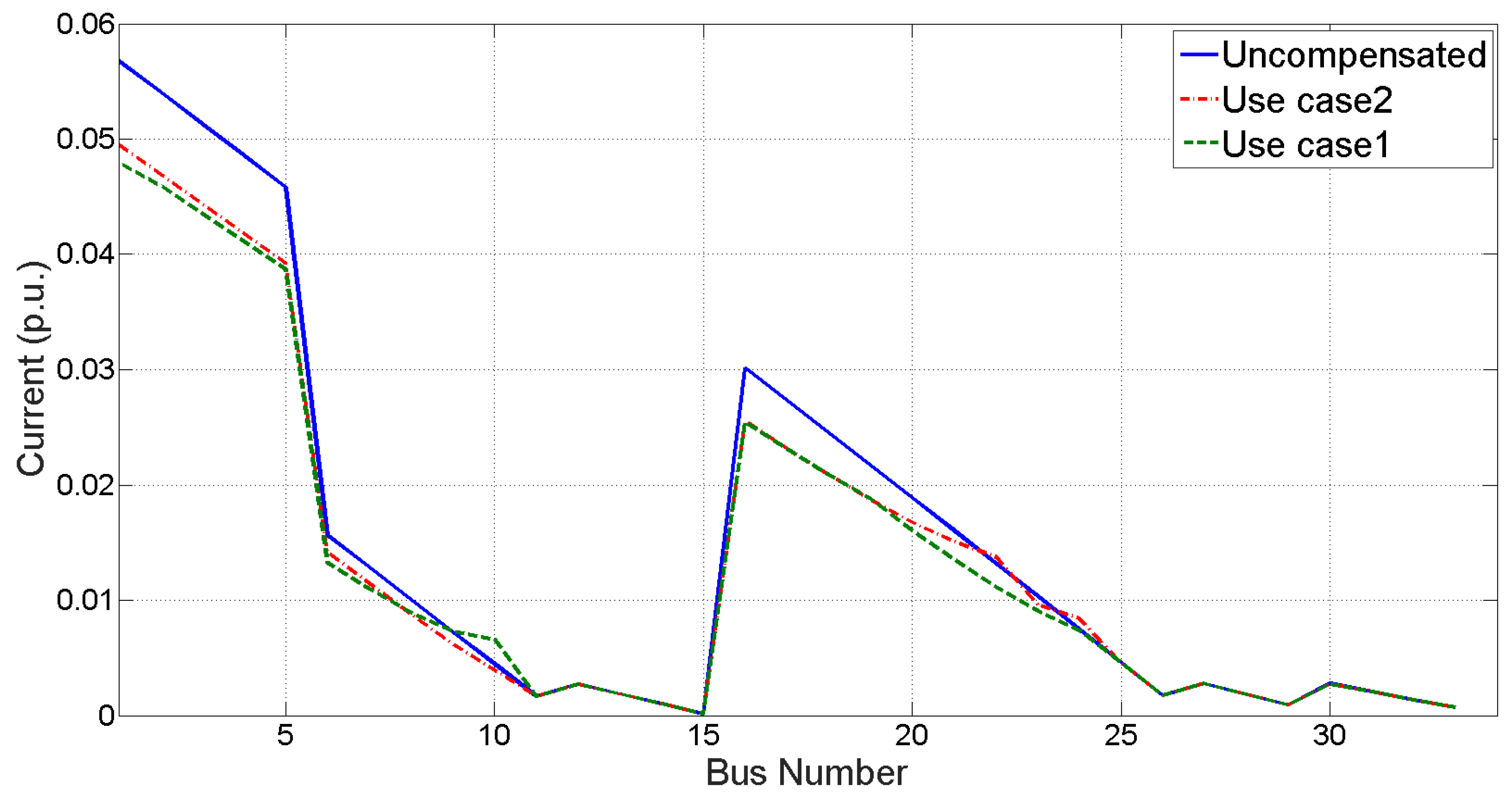
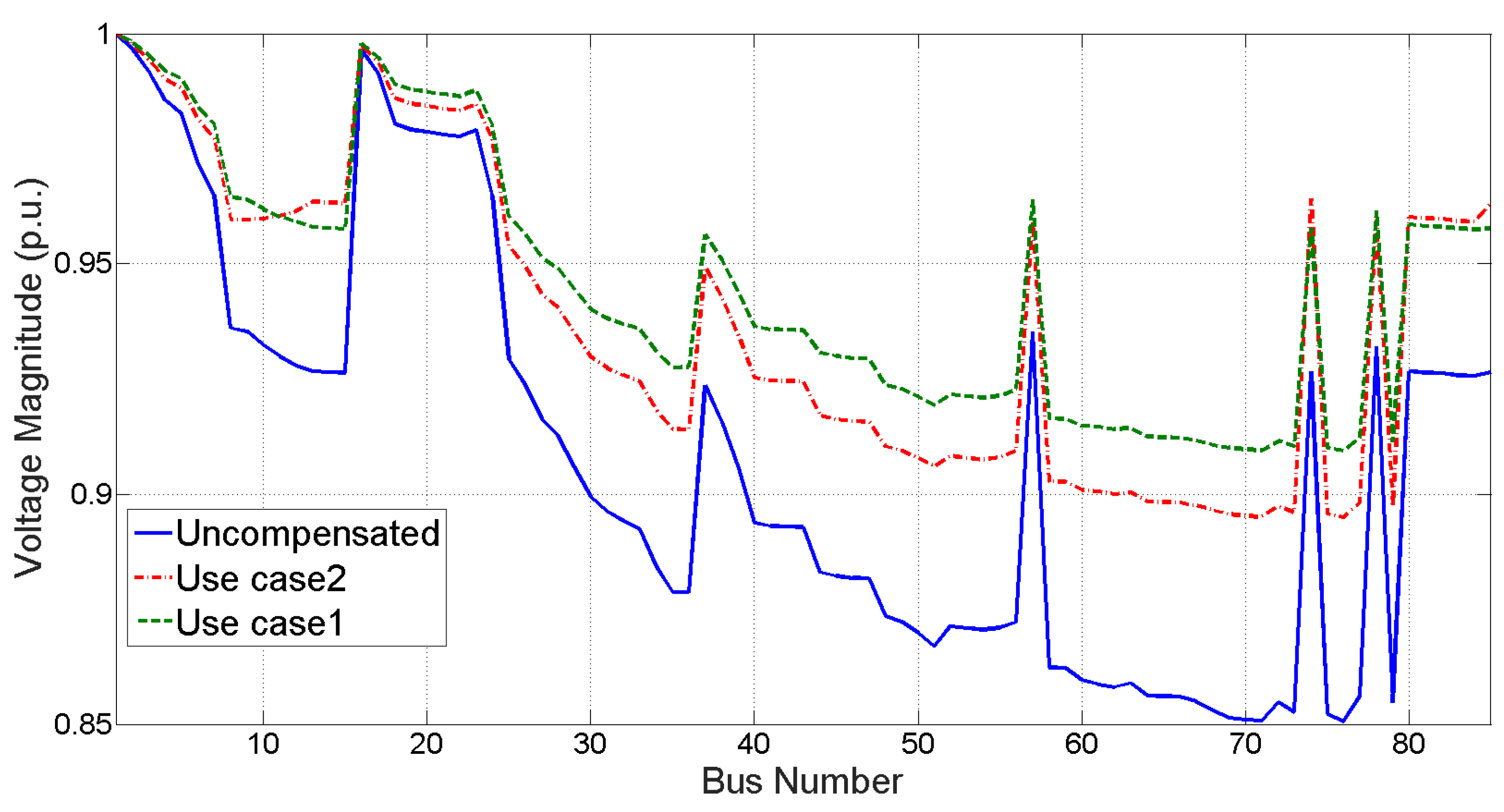
4.1. 34 and 85 Node RDNs – C S 1

For N 1 , the voltage profile has improved significantly after using the proposed capacitor placement, as shown in Table 2. Prior to compensation, minimum and maximum voltage in the network was 0.9411 pu at node 27 and 0.9941 pu at node 2, respectively. For use case 1, these values are improved to 0.9504 pu and 0.9954 pu, respectively. For use case 2, minimum voltage is improved to 0.9503 pu and maximum voltage is improved to 0.9949 pu. Voltage profile and line flow for N 1 are shown in Figure 6 and Figure 7, respectively. In these figure results of the uncompensated case, use case 1 and use case 2 are shown.
Initially the total annual cost of N 1 is USD 37,241/year (uncompensated) that is reduced to USD 26,655/year in use case 1 with USD 10,586.03/year of net saving, while for use case 2, it is reduced to USD 26,894/year with USD 10,347/year of net saving. From Table 2, Figure 6 and Figure 7, it is obvious that the results of use case 1 is better than use case 2. One reason for this can be the limitation on capacitor values in use case 2, i.e., the optimization algorithm is only allowed to select specified (commercially available) values of capacitors. It is obvious from Table 2 that the proposed method provided better results than PGSA [33], BFA [36], and GA [35].
The results of N 2 are presented in Table 3 for C S 1 , which are compared with other algorithms. As shown in Table 3, for use case 1, optimal placement of the capacitor is done at locations 27, 29, 30, 64, 51, 50, 67, 19, 46, and 80, with a 2134.5 kvar injection in the system. Similarly, for use case 2, capacitors are placed at locations 25, 48, 51, 64, 18, 68, 12, 61, and 44, with a 2250 kvar injection. The placement of these capacitors in N 2 minimized the active power loss from 319 to 140.8943 kW, which is a 55.85% reduction for use case 1, and to 145.20 kW for use case 2, which is a 54.504% reduction. Likewise, for both use cases of capacitors, reactive power losses reduced from 182 to 80.7297 kvar (55.68% reduction) for use case 1 and to 82.65 kvar (54.625% reduction) for use case 2, respectively. Comparative to other algorithms considered, the proposed method provides better results.
After optimizing the system with PSO, the total annual cost of the system is reduced to USD 23,670/year from USD 53,619/year in use case 1 with net savings of USD 29,950/year. For use case 2, the total annual cost of system is reduced to USD 24,394/year with savings of USD 29,224/year. It was also observed for this network that the results of use case 1 are better than use case 2 due to the limitation on capacitor values in use case 2. Voltage profile and line flow for 85 node RDN are shown in Figure 8 and Figure 9, respectively. Prior to compensation, it can be observed that the voltage at some buses violate the limits. These scenarios are improved after optimization and the constraints are satisfied. The maximum value of voltage is 0.9961 pu at node 2 and minimum voltage is 0.8505 pu at node 76. In use case 1, the maximum voltage is 0.9981 pu at node 2 and minimum voltage is 0.9100 pu at node 76. Similarly, for use case 2, the maximum voltage is improved from 0.9961 to 0.9979 pu at node 2 and minimum voltage is improved from 0.8505 to 0.9068 pu at node 7. In Figure 8, line flow of uncompensated and compensated cases are shown.

4.2. 34 and 85 Node RDNs – C S 2

For this case study, two scenarios are considered.
Scenario 1 ( S 1 ): optimization is conducted for the period of January to March. Capacitor locations and sizes are determined. After an increase in load, no variations in capacitor size and location are made. Based on these sizes and locations, the results are analyzed for coming seasons.
Scenario 2 ( S 2 ): optimization is conducted for the same duration of January to March. Capacitor locations and sizes are determined. After variations in loads in coming seasons, optimal sizes of capacitors are determined, and results are compared with those of S 1 .
Table 4 and Table 5 contain the data for uncompensated N 1 and N 2 for C S 2 , respectively. For N 1 , results of seasonal load are displayed in Table 6 according to S 1 . For the January to March season, optimal capacitor placement is performed and kept for other forthcoming seasons. For use case 1, capacitors of sizes 150, 481, 836, and 539 are placed at locations 19, 21, 24, and 8. The active power loss is reduced to 158 from 221 kW—a 28.52% reduction. Similarly, reactive power loss has been reduced to 43 from 65.1007 kvar, i.e., a 33% reduction. Capacitor sizes for use case 2 are 300, 300, 600, and 600, placed at locations 17, 20, 23, and 8. The active power losses are reduced to 160 from 221 kW, i.e., a 27.88% reduction. Similarly, reactive power loss was reduced to 43 from 65.23 kvar, i.e., 30.52% reduction.
For April–June, the load is increased to 1.8 times of the January–March load. With an increase in load, the losses also increased as shown in Table 4. Keeping sizes and locations of capacitors fixed at the January-March season results, it is observed that the active power loss reduction is 8% for use case 1 and 7.7% for use case 2. Similarly, reactive power loss reduction is 9.7% for use case 1 and 8.7% for use case 2. Consequently, the annual cost reduction is USD 120,883/year in use case 1. These results highlight the need for optimal capacitor placement in each season according to the respective load. Based on this observation, the results are improved in S 2 .
The outcomes of the seasonal load profile for N 1 are detailed in the Table 7 for S 2 . The increasing load alternatively increased system power losses, requiring optimization at each season. After the load change, according to the season, the results improved significantly if the capacitor placement was re-analyzed for updated network conditions. For example, when the load increased to 1.8 times of January–March in the second quarter, the losses increased to 782.1081 from 221.67 kW and to 229.309 kvar from 65.1007 kvar. To achieve better loss reduction and, hence, better annual savings, the sizes of the capacitors need to be updated only while installing them at similar locations, as in S 1 . The updated sizes are now 160, 1134, 1200, and 853, injecting the total of 3347 kvar. It can be seen in Table 7 that the active power loss is reduced to 28.99%, which is only 8% in S 1 . Similarly, a reduction in reactive power loss is 28.75%, which is 7.7% in S 1 for use case 1. Likewise, results of use case 2 for S 2 are better than that of S 1 , as shown in Table 7. Net savings for use case 1 is USD 10,511 and USD 38,101/year for S 1 and S 2 , respectively.
The same procedure is done for N 2 . The C S 2 results of N 2 for each scenario are shown in Table 8 and Table 9, respectively. In S 1 , the annual cost is significantly reduced by placing optimal capacitors of sizes 150, 150, 203, 439, 295, 150,150, 150,161, and 286 at optimal locations (27, 29, 30, 64, 51, 50, 67, 19, 46, and 80). The active and reactive power losses are reduced to 55.85% and 55.68% for use case 1, respectively. This loss reduction only corresponds to 12% and 12.5% for active and reactive losses, respectively, for the April–June season, as shown in Table 8. Consequently, the annual cost reduction is USD 70,058/year for use case 1. Due to reasons discussed earlier, the S 2 produced improved results and are discussed in Table 9.
Results of N 2 for S 2 are shown in Table 9. For April–June season, sizes of optimal capacitors are updated at the same location. Moreover, for N 2 , some new capacitors are needed to be installed at new locations for this specific season to ensure better annual cost savings in both use cases. Unlike S 1 , after optimization, the reduction in active power loss is 30.8%, which is 12% in case of S 1 (use case 1). Moreover, for (April–June) reactive power loss is reduced to 27.9%, which is 12.5% in case of S 1 . Comparing both scenarios, results of S 2 are better than S 1 in all aspects shown in Table 9. Unlike N 1 , installation of capacitors at new location in N 2 may need better optimization. However, as per common practice, the capacitors are installed at various locations and brought into the operation as and when needed.

5. Conclusions

In this work, we presented the annual costs of operations and reinforcement with capacitors, to reduce losses and improve the voltage profile, while keeping the network constraints. It is observed that the annual savings are significant if the proposed method is utilized for installation of the capacitors in RDNs. Moreover, system performance in terms of voltage profile, line flows, and losses improved significantly compared to recent methods presented in the literature. The ranking of buses, based on loss sensitivity, with respect to the voltage and reactive power injection at the neighboring buses, has reduced the search space for PSO without compromising the quality of results. Net annual saving for 34- and 85-node RDNs with static loads can be as high as USD 10,586 and USD 29,950/year, respectively. For seasonal load profiles, net annual savings are recorded to be USD 10511 and USD 38,101/year for the 34-node RDNs in scenarios 1 and 2, respectively. Similarly, for the 85-node RDN, USD 30,024 and USD 74,446/year is the net annual saving in scenarios 1 and 2, respectively. we conclude that better net annual cost savings is expected if the capacitor sizes and locations are updated according to seasonal load variations. Moreover, the method proposed in this work produced better results in comparison to recent novel methods. The work can be extended by considering other variables, such as the operation and maintenance costs.

Author Contributions

Conceptualization, M.A.; data curation, M.B.; formal analysis, M.S. and M.A.; funding acquisition, S.B.H. and S.S.A.A.; project administration, B.U.; supervision, M.S.; writing—original draft, M.S.; writing—review and editing, B.U., S.B.H. and S.S.A.A. All authors have read and agreed to the published version of the manuscript.

Funding

This research was supported in part by COMSATS University Islamabad, Abbottabad Campus, Pakistan and Universiti Teknologi PETRONAS JRP grant 015ME0-228.

Institutional Review Board Statement

Not applicable.

Informed Consent Statement

Not applicable.

Acknowledgments

The authors acknowledge the support from Institute of Health & Analytics, Universiti Teknologi PETRONAS, Malaysia.

Conflicts of Interest

The authors declare no conflict of interest.

Abbreviations

The following abbreviations are used in this manuscript:
FTotal cost per year ($/Year)
C p Cost of per unit active power loss per year ($/kW-Year)
C q Cost of per unit reactive power loss per year ($/kvar-Year)
C C Purchasing and installation cost of capacitor installed ($/kvar)
P l o s s T o t Total active power loss kW
Q l o s s T o t Total reactive power loss kvar
Q C T o t Total injected reactive power (kvar)
Q c q Reactive power injection at location q
N b Number of nodes in the system
N c Number of capacitors to be placed in system
N C m a x Maximum permissible number of capacitors to be placed in the system
nLife expectancy of the capacitors
Q L T o t Total required reactive power by load
V q Bus voltage at node q
V q m i n Minimum voltage at node q
V q m a x Maximum voltage at node q
Q C q Reactive power injection at node q
Q C q m i n Minimum reactive power injection at node q
Q C q m a x Maximum reactive power injection at node q
P L q Total active power loads beyond the bus q
Q L q Total reactive power loads beyond bus q
P l o s s k Total active power loss in line k
Q l o s s k Total reactive power loss in line k
i k Total current flowing over the line k
R k Total resistance of the line k
X k Total reactance of the line k
X i k Initial position of i t h particle in k t h iteration
V e l i k Initial velocity of i t h particle in k t h iteration
V e l i k + 1 Modified velocity of i t h particle in k + 1 t h iteration
X i k + 1 Modified position of i t h particle in k + 1 t h iteration
P b e s t p Personal best position of the particle
G b e s t p Global best position of the particle
wThe inertia weight
c 1 Constant for acceleration
c 2 Constant for acceleration
r 1 Random numbers between 0 and 1
r 2 Random numbers between 0 and 1

References

  1. Mtonga, T.P.; Kaberere, K.K.; Irungu, G.K. Optimal Shunt Capacitors’ Placement and Sizing in Radial Distribution Systems Using Multiverse Optimizer. IEEE Can. J. Electr. Comput. Eng. 2021, 44, 10–21. [Google Scholar] [CrossRef]
  2. Safayet, A.; Fajri, P.; Husain, I. Reactive power management for overvoltage prevention at high PV penetration in a low-voltage distribution system. IEEE Trans. Ind. Appl. 2017, 53, 5786–5794. [Google Scholar] [CrossRef]
  3. Abou El-Ela, A.A.; El-Sehiemy, R.A.; Abbas, A.S. Optimal placement and sizing of distributed generation and capacitor banks in distribution systems using water cycle algorithm. IEEE Syst. J. 2018, 12, 3629–3636. [Google Scholar] [CrossRef]
  4. Shahzad, M.; Akram, W.; Arif, M.; Khan, U.; Ullah, B. Optimal Siting and Sizing of Distributed Generators by Strawberry Plant Propagation Algorithm. Energies 2021, 14, 1744. [Google Scholar] [CrossRef]
  5. Ismail, B.; Wahab, N.I.A.; Othman, M.L.; Radzi, M.A.M.; Vijyakumar, K.N.; Naain, M.N.M. A comprehensive review on optimal location and sizing of reactive power compensation using hybrid-based approaches for power loss reduction, voltage stability improvement, voltage profile enhancement and loadability enhancement. IEEE Access 2020, 8, 222733–222765. [Google Scholar] [CrossRef]
  6. Srikanth, T.; Selvi, S.C.; Pushya, V.P. Optimal placement of static VAR compensator (SVC) in power system along with wind power generation. In Proceedings of the 2017 IEEE International Conference on Electrical, Instrumentation and Communication Engineering (ICEICE), Karur, India, 27–28 April 2017; pp. 1–6. [Google Scholar]
  7. Mohanan, V.A.V.; Mareels, I.M.; Evans, R.J.; Kolluri, R.R. Stabilising influence of a synchronous condenser in low inertia networks<? show [AQ="" ID=" Q1]"? IET Gener. Transm. Distrib. 2020, 14, 3582–3593. [Google Scholar]
  8. Hannan, M.A.; Islam, N.N.; Mohamed, A.; Lipu, M.S.H.; Ker, P.J.; Rashid, M.M.; Shareef, H. Artificial intelligent based damping controller optimization for the multi-machine power system: A review. IEEE Access 2018, 6, 39574–39594. [Google Scholar] [CrossRef]
  9. Jahromi, M.H.M.; Dehghanian, P.; Khademi, M.R.M.; Jahromi, M.Z. Reactive Power Compensation and Power Loss Reduction using Optimal Capacitor Placement. In Proceedings of the 2021 IEEE Texas Power and Energy Conference (TPEC), College Station, TX, USA, 2–5 February 2021; pp. 1–6. [Google Scholar]
  10. Díaz, P.; Pérez-Cisneros, M.; Cuevas, E.; Camarena, O.; Martinez, F.A.F.; González, A. A swarm approach for improving voltage profiles and reduce power loss on electrical distribution networks. IEEE Access 2018, 6, 49498–49512. [Google Scholar] [CrossRef]
  11. Noori, A.; Zhang, Y.; Nouri, N.; Hajivand, M. Multi-Objective Optimal Placement and Sizing of Distribution Static Compensator in Radial Distribution Networks With Variable Residential, Commercial and Industrial Demands Considering Reliability. IEEE Access 2021, 9, 46911–46926. [Google Scholar] [CrossRef]
  12. Das, S.; Das, D.; Patra, A. Operation of distribution network with optimal placement and sizing of dispatchable DGs and shunt capacitors. Renew. Sustain. Energy Rev. 2019, 113, 109219. [Google Scholar] [CrossRef]
  13. Singh, S.P.; Prakash, T.; Singh, V.; Babu, M.G. Analytic hierarchy process based automatic generation control of multi-area interconnected power system using Jaya algorithm. Eng. Appl. Artif. Intell. 2017, 60, 35–44. [Google Scholar] [CrossRef]
  14. Sinha, A.; Malo, P.; Deb, K. A review on bilevel optimization: From classical to evolutionary approaches and applications. IEEE Trans. Evol. Comput. 2017, 22, 276–295. [Google Scholar] [CrossRef]
  15. Shahzad, M.; Shafiullah, Q.; Akram, W.; Arif, M.; Ullah, B. Reactive Power Support in Radial Distribution Network Using Mine Blast Algorithm. Elektron. Elektrotechnika 2021, 27, 33–40. [Google Scholar] [CrossRef]
  16. Elsayed, A.M.; Mishref, M.M.; Farrag, S.M. Optimal allocation and control of fixed and switched capacitor banks on distribution systems using grasshopper optimisation algorithm with power loss sensitivity and rough set theory. IET Gener. Transm. Distrib. 2019, 13, 3863–3878. [Google Scholar] [CrossRef]
  17. Jafari, A.; Ganjehlou, H.G.; Khalili, T.; Mohammadi-Ivatloo, B.; Bidram, A.; Siano, P. A two-loop hybrid method for optimal placement and scheduling of switched capacitors in distribution networks. IEEE Access 2020, 8, 38892–38906. [Google Scholar] [CrossRef]
  18. Tamilselvan, V.; Jayabarathi, T.; Raghunathan, T.; Yang, X.S. Optimal capacitor placement in radial distribution systems using flower pollination algorithm. Alex. Eng. J. 2018, 57, 2775–2786. [Google Scholar] [CrossRef]
  19. Almabsout, E.A.; El-Sehiemy, R.A.; An, O.N.U.; Bayat, O. A hybrid local search-genetic algorithm for simultaneous placement of DG units and shunt capacitors in radial distribution systems. IEEE Access 2020, 8, 54465–54481. [Google Scholar] [CrossRef]
  20. Hussain, A.N.; Shakir Al-Jubori, W.K.; Kadom, H.F. Hybrid design of optimal capacitor placement and reconfiguration for performance improvement in a radial distribution system. J. Eng. 2019, 2019, 1696347. [Google Scholar] [CrossRef] [Green Version]
  21. Reddy, A.; Reddy, M.D. Optimal Capacitor allocation for the reconfigured Network using Ant Lion Optimization algorithm. Int. J. Appl. Eng. Res. 2017, 12, 3084–3089. [Google Scholar] [CrossRef]
  22. Tolba, M.A.; Diab, A.A.Z.; Tulsky, V.N.; Abdelaziz, A.Y. VLCI approach for optimal capacitors allocation in distribution networks based on hybrid PSOGSA optimization algorithm. Neural Comput. Appl. 2019, 31, 3833–3850. [Google Scholar] [CrossRef]
  23. Diab, A.A.Z.; Tolba, M.A.; Tulsky, V.N. A new hybrid PSOGSA algorithm for optimal allocation and sizing of capacitor banks in RDS. In Proceedings of the 2017 IEEE Conference of Russian Young Researchers in Electrical and Electronic Engineering (EIConRus), St. Petersburg and Moscow, Russia, 1–3 February 2017; pp. 1496–1501. [Google Scholar]
  24. Kennedy, J.; Eberhart, R. Particle swarm optimization. In Proceedings of the ICNN’95-International Conference on Neural Networks, Perth, WA, Australia, 27 November—1 December 1995; Volume 4, pp. 1942–1948. [Google Scholar]
  25. Rani, B.J.; Reddy, A.S. Optimal allocation and sizing of multiple DG in radial distribution system using binary particle swarm optimization. Int. J. Intell. Eng. Syst. 2019, 12, 290–299. [Google Scholar] [CrossRef]
  26. Veerasamy, V.; Wahab, N.I.A.; Ramachandran, R.; Othman, M.L.; Hizam, H.; Irudayaraj, A.X.R.; Guerrero, J.M.; Kumar, J.S. A Hankel matrix based reduced order model for stability analysis of hybrid power system using PSO-GSA optimized cascade PI-PD controller for automatic load frequency control. IEEE Access 2020, 8, 71422–71446. [Google Scholar] [CrossRef]
  27. Llerena-Pizarro, O.; Proenza-Perez, N.; Tuna, C.E.; Silveira, J.L. A PSO-BPSO technique for hybrid power generation system sizing. IEEE Lat. Am. Trans. 2020, 18, 1362–1370. [Google Scholar] [CrossRef]
  28. Yousaf, S.; Mughees, A.; Khan, M.G.; Amin, A.A.; Adnan, M. A Comparative Analysis of Various Controller Techniques for Optimal Control of Smart Nano-Grid Using GA and PSO Algorithms. IEEE Access 2020, 8, 205696–205711. [Google Scholar] [CrossRef]
  29. Kefale, H.A.; Getie, E.M.; Eshetie, K.G. Optimal design of grid-connected solar photovoltaic system using selective particle swarm optimization. Int. J. Photoenergy 2021, 2021. [Google Scholar] [CrossRef]
  30. Ahshan, R. Analysis of Loss Reduction Techniques for Low Voltage Distribution Network. J. Eng. Res. 2020, 17, 100–111. [Google Scholar]
  31. Amara, T.; Asefi, S.; Adewuyi, O.B.; Ahmadi, M.; Yona, A.; Senjyu, T. Technical and economic performance evaluation for efficient capacitors sizing and placement in a real distribution network. In Proceedings of the 2019 IEEE Student Conference on Research and Development (SCOReD), Bandar Seri Iskandar, Malaysia, 15–17 October 2019; pp. 100–105. [Google Scholar]
  32. Abou El-Ela, A.A.; El-Sehiemy, R.A.; Kinawy, A.M.; Mouwafi, M.T. Optimal capacitor placement in distribution systems for power loss reduction and voltage profile improvement. IET Gener. Transm. Distrib. 2016, 10, 1209–1221. [Google Scholar] [CrossRef]
  33. Rao, R.S.; Narasimham, S.; Ramalingaraju, M. Optimal capacitor placement in a radial distribution system using plant growth simulation algorithm. Int. J. Electr. Power Energy Syst. 2011, 33, 1133–1139. [Google Scholar] [CrossRef] [Green Version]
  34. Raju, M.R.; Murthy, K.R.; Ravindra, K. Direct search algorithm for capacitive compensation in radial distribution systems. Int. J. Electr. Power Energy Syst. 2012, 42, 24–30. [Google Scholar] [CrossRef]
  35. Reddy, V.; Sydulu, M. 2Index and GA based optimal location and sizing of distribution system capacitors. In Proceedings of the 2007 IEEE Power Engineering Society General Meeting, Tampa, FL, USA, 24–28 June 2007; pp. 1–4. [Google Scholar]
  36. Tabatabaei, S.; Vahidi, B. Bacterial foraging solution based fuzzy logic decision for optimal capacitor allocation in radial distribution system. Electr. Power Syst. Res. 2011, 81, 1045–1050. [Google Scholar] [CrossRef]
  37. Upper, N.; Hemeida, A.M.; Ibrahim, A. Moth-flame algorithm and loss sensitivity factor for optimal allocation of shunt capacitor banks in radial distribution systems. In Proceedings of the 2017 Nineteenth International Middle East Power Systems Conference (MEPCON), Cairo, Egypt, 19–21 December 2017; pp. 851–856. [Google Scholar]
  38. Jumani, T.A.; Mustafa, M.W.; Alghamdi, A.S.; Rasid, M.M.; Alamgir, A.; Awan, A.B. Swarm intelligence-based optimization techniques for dynamic response and power quality enhancement of AC microgrids: A comprehensive review. IEEE Access 2020, 8, 75986–76001. [Google Scholar] [CrossRef]
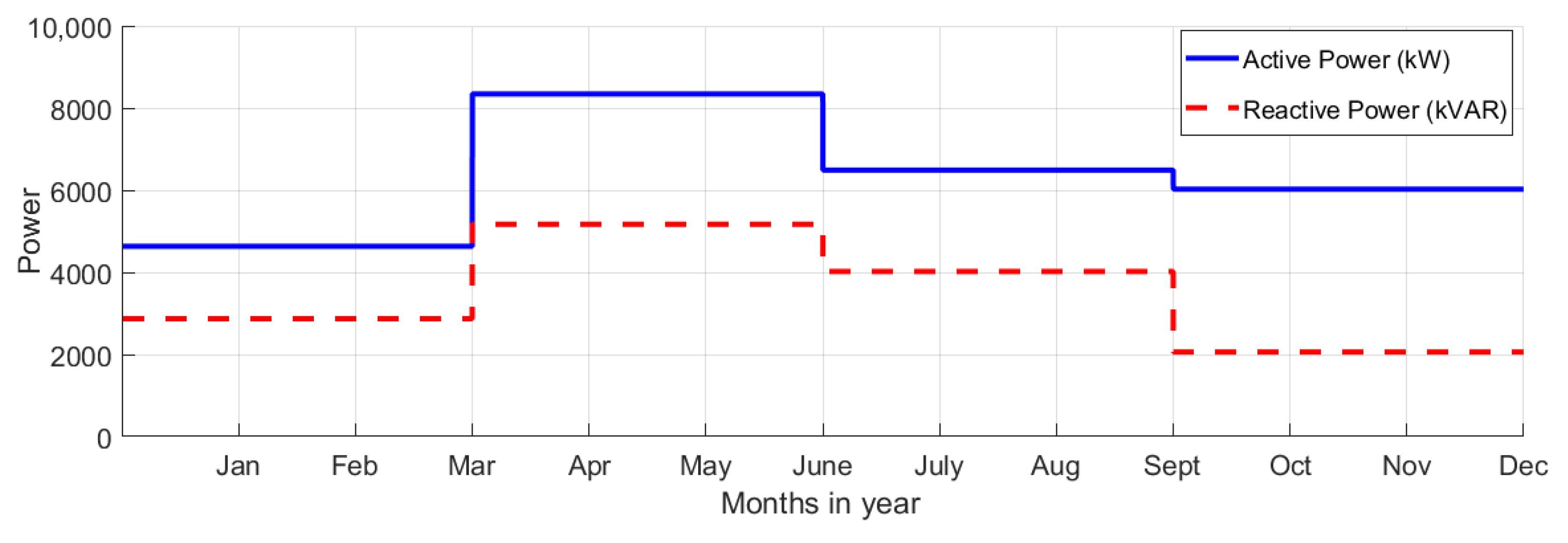
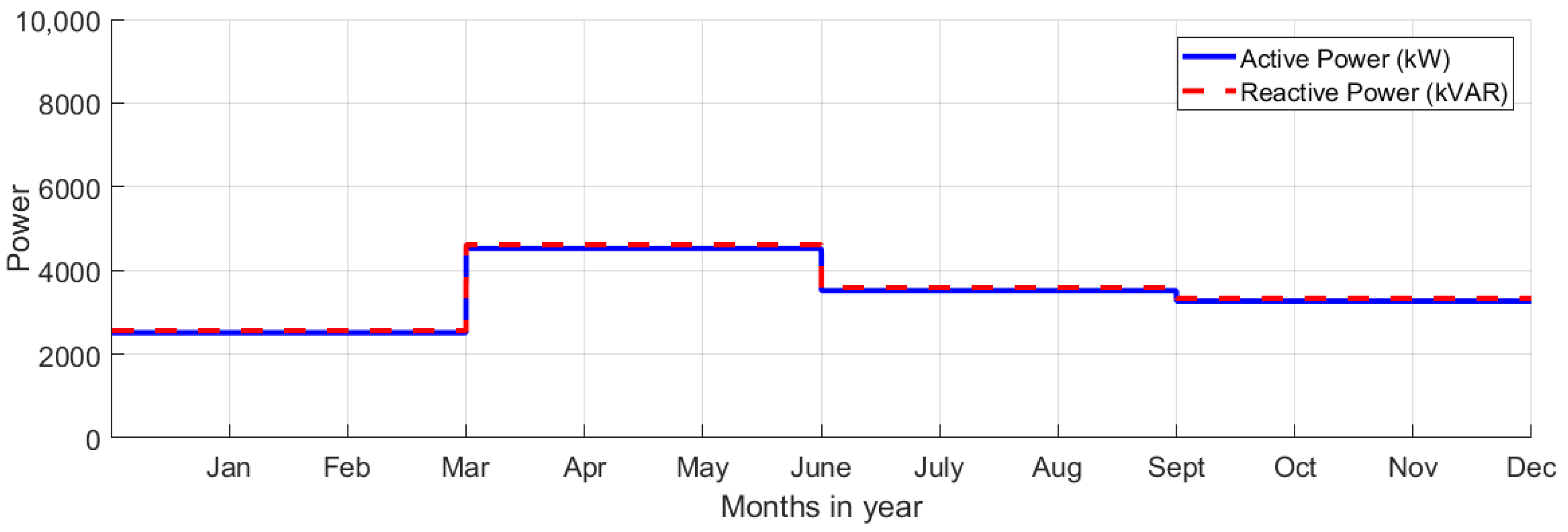
Figure 1. Two nodes representation of distribution system.
Applsci 11 11840 g001
Figure 2. Movement of a single particle in swarm.
Applsci 11 11840 g002
Figure 3. Flow chart for the proposed method.
Applsci 11 11840 g003
Figure 4. Seasonal load profile for N 1 .
Applsci 11 11840 g004
Figure 5. Seasonal load profile for N 2 .
Applsci 11 11840 g005
Figure 6. Voltage profile for N 1 in C S 1 .
Applsci 11 11840 g006
Figure 7. Line flow for N 1 in C S 1 .
Applsci 11 11840 g007
Figure 8. Voltage profile for N 2 in C S 1 .
Applsci 11 11840 g008
Figure 9. Line flow for N 2 in C S 1 .
Applsci 11 11840 g009
Table 1. Seasonal load profile for both networks.
MonthsActive Load (kW)Reactive Load (kvar)
Network N 1 N 2 N 1 N 2
January–March4636251428732564
April–June8345452551724616
July–September6491352040223590
October–December6027326820613333
Table 2. Results comparison of N 1 for C S 1 .
ItemsUncom-
Pensated
Compensated
PGSABFAGAACO AlgorithmProposed Algorithm
Use Case1Use Case2Use Case1Use Case2
kvar injected at node-1200 (19)
200 (20)
639 (22)
600 (9)
900 (22)
1629 (7)645 (9)
719 (22)
665 (25)
450 (9)
450 (19)
450 (25)
150 (19)
481 (21)
836 (24)
539 (8)
300 (17)
300 (20)
600 (23)
600 (8)
Total kvar injected-2039150016292029195020071800
Active loss (kW)221.7169.1169.1168.9162.7164.5158.7160.1
Reactive loss (kvar)65.1-----43.345.2
Active loss reduction (%)-23.723.723.826.625.828.527.9
Reactive loss reduction (%)------33.430.5
V m i n at node0.94 (27)0.95 (27)0.94 (27)0.95 (27)0.95 (27)0.95 (27)0.95 (27)0.95 (27)
V m a x at node0.99 (2)0.99 (2)0.99 (2)0.99 (2)0.99 (2)0.99 (2)0.99 (2)0.99 (2)
Annual cost USD ($)/year37,24128,42028,40428,38427,33027,63726,65526,894
Capacitor cost UD ($)/year-1019.5750814.510149751003.5900
Net saving USD ($)/year-882188378857991196041058610,347
Table 3. Results comparison of N 2 for C S 1 .
ItemsUncom-
Pensated
Compensated
PGSADSAGAACO AlgorithmProposed Algorithm
Use Case1Use Case2Use Case1Use Case2
kvar injected at node-200 (7)
1200 (8)
908 (58)
150 (6)
150 (8)
150 (14)
150 (17)
150 (18)
150 (20)
150 (26)
150 (30)
450 (37)
150 (57)
150 (61)
150 (66)
300 (69)
150 (80)
48.4 (26)
214 (28)
103.1 (37)
120.3 (38)
178 (39)
100 (51)
212.5 (54)
101.5 (55)
4.6 (59)
157 (60)
112.5 (61)
104 (62)
9.3 (66)
100 (69)
67 (72)
112.5 (74)
71.9 (76)
356.2 (80)
31.2 (82)
186 (4)
150 (7)
210 (9)
10 (13)
280 (18)
320 (26)
250 (31)
205 (35)
200 (53)
220 (61)
330 (68)
196 (80)
150 (7)
300 (8)
300 (19)
300 (27)
300 (32)
300 (48)
300 (61)
300 (68)
300 (80)
150(27)
150 (29)
203.5 (30)
439.4 (64)
295 (51)
150 (50)
150 (67)
150 (19)
161 (46)
286 (80)
300(25)
150 (48)
600 (51)
150 (64)
300 (18)
150 (68)
300 (12)
150 (61)
150 (44)
Total kvar injected-230825502207272625502134.92250
Active loss (kW)319174.9144.0146143.3143.9140.9145.2
Reactive loss (kvar)182-----80.782.6
Active loss reduction (%)-4454.453.754.654.455.854.5
Reactive loss reduction (%)------55.754.6
V m i n at node0.85 (76)0.90 (54)0.92 (54)0.92 (55)0.92 (54)0.92 (27)0.91 (76)0.91 (76)
V m a x at node0.99 (2)0.99 (2)0.99 (2)0.99 (2)0.99 (2)0.99 (2)0.99 (2)0.99 (2)
Annual cost USD ($)/year53,61929,38524,19424,53824,08224,17123,67024,394
Capacitor cost USD ($)/year-115412751103136312751067.41125
Net saving USD ($)/year-24,23429,42529,08129,53729,44829,94929,225
Table 4. Base data (uncompensated) of N 1 for C S 2 .
MonthsUncompensated
January–MarchApril–JuneJuly–SeptemberOctober–December
Active loss (kW)221.7782.1674523.5
Reactive loss (kvar)65.1229.3198153
Total cost (USD ($)/year)37,241131,394113,37287,991
V m i n at node0.94 (27)0.89 (27)0.88 (27)0.90 (27)
V m a x at node0.99 (2)0.99 (2)0.99 (2)0.99 (2)
Table 5. Base data (uncompensated) of N 2 for C S 2 .
MonthsUncompensated
January–MarchApril–JuneJuly–SeptemberOctober–December
Total active loss (kW)319.21436.9717.6595.7
Reactive loss (kvar)182.1810.9407.7338.9
Total cost (USD ($)/year)53,619.6241,406.4120,556.7100,082.8
V m i n at node0.85 (76)0.67 (76)0.77 (76)0.79 (76)
V m a x at node0.99 (2)0.99 (2)0.99 (2)0.99 (2)
Table 6. Results comparison of N 1 for C S 2 (Scenario 1).
MonthsCompensated
January–MarchApril–June (1.8)July–September (1.4)October–December (1.3)
Use CasesUse Case 1Use Case 2Use Case 1Use Case 2Use Case 1Use Case 2Use Case 1Use Case 2
kvar injected at node150 (19)
481 (21)
836 (24)
539 (8)
300 (17)
300 (20)
600 (23)
600 (8)
150 (19)
481 (21)
836 (24)
539 (8)
300 (17)
300 (20)
600 (23)
600 (8)
150 (19)
481 (21)
836 (24)
539 (8)
300 (17)
300 (20)
600 (23)
600 (8)
150 (19)
481 (21)
836 (24)
539 (8)
300 (17)
300 (20)
600 (23)
600 (8)
Total kvar injected20071800200718002007180020071800
Active loss (kW)158160719722611613460462
Reactive loss (kvar)43.345.220720917678131133
Active loss reduction (%)28.527.987.79.591311.7
Reactive loss reduction (%)33.430.59.78.711101413
V m i n at node0.95 (27)0.95 (27)0.79 (27)0.77 (27)0.80 (27)0.80 (27)0.86 (27)0.82 (27)
V m a x at node0.99 (2)0.99 (2)0.90 (2)0.90 (2)0.93 (2)0.92 (2)0.94 (2)0.94 (2)
Annual cost (USD ($)/year)26,65526,894120,883121,277102,602103,16976,55377,697
Capacitor cost (USD ($)/year)1003900100390010039001003900
Net saving (USD ($)/year)10,58610,34710,51110,11710,77710,20311,43810,294
Table 7. Results comparison of N 1 for C S 2 (Scenario 2).
MonthsCompensated
January–MarchApril–June (1.8)July–September (1.4)October–December (1.3)
Use CasesUse Case 1Use Case 2Use Case 1Use Case 2Use Case 1Use Case 2Use Case 1Use Case 2
kvar injected at node150 (19)
481 (21)
836 (24)
539 (8)
300 (17)
300 (20)
600 (23)
600 (8)
160 (19)
1134 (21)
1200 (24)
853 (8)
600 (17)
600 (20)
600 (23)
600 (8)
426 (19)
475 (21)
722 (24)
723 (8)
450 (17)
450 (20)
600 (23)
600 (8)
445 (19)
353 (21)
602 (24)
589 (8)
450 (17)
600 (20)
300 (23)
450 (8)
Total kvar injected20071800334724002350.9210019901800
Active loss (kW)158160555557479497370375
Reactive loss (kvar)43.345.2156.5162.8140.3143105109
Active loss reduction (%)28.527.928.928.728.926.229.228.2
Reactive loss reduction (%)33.430.531.728.929.127.431.628.7
V m i n at node0.95 (27)0.95 (27)0.91 (27)0.90 (27)0.90 (27)0.89 (27)0.91 (27)0.90 (27)
V m a x at node0.99 (2)0.99 (2)0.99 (2)0.99 (2)0.99 (2)0.99 (2)0.99 (2)0.99 (2)
Annual cost (USD ($)/year)26,65526,89493,29293,61380,50583,62462,25263,111
Capacitor cost (USD ($)/year)10039001673120011751050995900
Net saving (USD ($)/year)10,58610,34738,10137,78132,86629,74825,74024,880
Table 8. Results comparison of N 2 for C S 2 (Scenario 1).
MonthsCompensated
January–MarchApril–June (1.8)July–September (1.4)October–December (1.3)
Use CasesUse Case 1Use Case 2Use Case 1Use Case 2Use Case 1Use Case 2Use Case 1Use Case 2
kvar injected at node150 (27)
150 (29)
203 (30)
439 (64)
295 (51)
150 (50)
150 (67)
150 (19)
161 (46)
286 (80)
300 (25)
150 (48)
600 (51)
150 (64)
300 (18)
150 (68)
300 (12)
150 (61)
150 (44)
150 (27)
150 (29)
203 (30)
439 (64)
295 (51)
150 (50)
150 (67)
150 (19)
161 (46)
286 (80)
300 (25)
150 (48)
600 (51)
150 (64)
300 (18)
150 (68)
300 (12)
150 (61)
150 (44)
150 (27)
150 (29)
203 (30)
439 (64)
295 (51)
150 (50)
150 (67)
150 (19)
161 (46)
286 (80)
300 (25)
150 (48)
600 (51)
150 (64)
300 (18)
150 (68)
300 (12)
150 (61)
150 (44)
150 (27)
150 (29)
203 (30)
439 (64)
295 (51)
150 (50)
150 (67)
150 (19)
161 (46)
286 (80)
300 (25)
150 (48)
600 (51)
150 (64)
300 (18)
150 (68)
300 (12)
150 (61)
150 (44)
Total kvar injected21342250213422502134225021342250
Active loss (kW)140.9145.2125712623341334630893094
Reactive loss (kvar)80.782.67087103488349032313233
Active loss reduction (%)55.854.5121224.924.53029
Reactive loss reduction (%)55.754.612.512.32524.73029
V m i n at node0.91 (76)0.90 (76)0.79 (76)0.68 (76)0.70 (76)0.70 (76)0.70 (76)0.73 (76)
V m a x at node0.99 (2)0.99 (2)0.89 (2)0.89 (2)0.87 (2)0.83 (2)0.88 (2)0.87 (2)
Annual cost (USD ($)/year)23,67024,394212,438212,43890,53891,12070,05871,059
Capacitor cost (USD ($)/year)10671125106711251067112510671125
Net saving (USD ($)/year)29,95029,22528,96828,96830,01829,43630,02429,023
Table 9. Results comparison of N 2 for C S 2 (Scenario 2).
MonthsCompensated
Jan-MarchApril–June (1.8)July–September (1.4)October–December (1.3)
Use CasesUse Case 1Use Case 2Use Case 1Use Case 2Use Case 1Use Case 2Use Case 1Use Case 2
kvar injected at node150 (27)
150 (29)
203 (30)
439 (64)
295 (51)
150 (50)
150 (67)
150 (19)
161 (46)
286 (80)
300(25)
150 (48)
600 (51)
150 (64)
300 (18)
150 (68)
300 (12)
150 (61)
150 (44)
300 (27)
150 (29)
1200 (30)
446 (64)
330 (51)
179 (50)
465 (67)
150 (19)
287 (46)
270 (80)
1046 (35)
150 (45)
1200 (68)
482 (10)
150 (17)
740 (9)
600 (25)
300 (48)
600 (51)
300 (64)
600 (18)
600 (68)
600 (12)
600 (61)
600 (44)
150 (50)
150 (67)
150 (19)
600 (80)
150 (2)
150 (27)
205 (29)
212 (30)
511 (64)
299 (51)
150 (50)
150 (67)
150 (19)
372 (46
363 (80)
875 (35)
150 (45)
1168 (68)
190 (60)
150 (17)
600 (25)
150 (48)
600 (51)
600 (64)
450 (18)
150 (68)
600 (12)
600 (61)
150 (44)
150 (50)
600 (80)
150 (27)
556 (29)
366 (30)
632 (64)
401 (51)
210 (50)
150 (19)
906 (80)
297 (57)
150 (25)
300 (48)
600 (51)
150 (64)
150 (18)
150 (68)
300 (12)
600 (61)
150 (44)
150 (50)
150 (61)
Total kvar injected21342250754560005096465036682850
Active loss (kW)1401459931119387410273289
Reactive loss (kvar)8082584679223237159164
Active loss reduction (%)55.855.530.822.146425451
Reactive loss reduction (%)55.754.628.022.145415251
V m i n at node0.91 (76)0.90 (76)0.91 (76)0.90 (76)0.90 (76)0.90 (76)0.90 (76)0.90 (76)
V m a x at node0.99 (2)0.99 (2)0.99 (2)0.99 (2)0.99 (2)0.99 (2)0.99 (2)0.99 (2)
Annual cost (USD ($)/year)23,67024,394166,960188,02065,03769,01545,86248,627
Capacitor cost (USD ($)/year)106711253772.530002548232518341425
Net saving (USD ($)/year)29,95029,22574,44653,38355,51951,54154,22051,455
Publisher’s Note: MDPI stays neutral with regard to jurisdictional claims in published maps and institutional affiliations.

