Response-Only Parametric Estimation of Structural Systems Using a Modified Stochastic Subspace Identification Technique

Abstract

The present paper is a study of output-only modal estimation based on the stochastic subspace identification technique (SSI) to avoid the restrictions of well-controlled laboratory conditions when performing experimental modal analysis and aims to develop the appropriate algorithms for ambient modal estimation. The conventional SSI technique, including two types of covariance-driven and data-driven algorithms, is employed for parametric identification of a system subjected to stationary white excitation. By introducing the procedure of solving the system matrix in SSI-COV in conjunction with SSI-DATA, the SSI technique can be efficiently performed without using the original large-dimension data matrix, through the singular value decomposition of the improved projection matrix. In addition, the computational efficiency of the SSI technique is also improved by extracting two predictive-state matrixes with recursive relationship from the same original predictive-state matrix, and then omitting the step of reevaluating the predictive-state matrix at the next-time moment. Numerical simulations and experimental verification illustrate and confirm that the present method can accurately implement modal estimation from stationary response data only.

1. Introduction

The dynamic characteristics of a structural system, such as natural frequencies, damping ratios, and mode shapes, can be investigated through numerical and experimental analysis. The response of a structural system is measured with a known excitation in modal testing, which is usually performed under well-controlled laboratory conditions. However, performing experimental modal analysis in real operating conditions may be possible, even for large and complex mechanical systems with real boundary conditions [1,2]. The modal parameters obtained theoretically under the free boundary condition can be calculated by mathematical modeling to obtain the characteristics under arbitrary boundary constraints [3]. However, experimental results obtained under specified boundary conditions cannot be converted to other dynamic characteristics under the constraints of other boundaries. Therefore, it is difficult to perform modal testing under practical boundary conditions. The hammer excitation testing method is generally used to measure the frequency response function of the structural system, and then parametric estimation is performed to understand the dynamic characteristics of the structural system [4].

The system-identification methods described above are generally used to systematically determine or improve a mathematical model for a physical system and are implemented by measuring both observed structural excitation and corresponding response data. However, an obvious difference exists between the operating conditions of realistic structures in practical work and a controlled-environment laboratory in modal testing [5]. Dynamic characteristics cannot fully represent the system mode under real-world operating conditions; thus, it is necessary to study how to perform modal identification of systems in authentic operating environments [6].

Operational modal analysis [7], which is also called “ambient modal analysis”, or “output-only modal analysis” [8], is extensively used in modal estimation of large structures under environmental and operational loads [9], such as vehicle suspension systems [10], offshore wind power facilities [11], and stadium structures [12]. Many identification methods have been extensively employed for modal extraction based on ambient response. In 1993, the so-called natural excitation technique (NExT) was proposed and initially used for modal estimation of structures in wind engineering, by assuming that ambient excitation is stationary white noise [13]. It was employed to replace free or impulse response in conventional modal estimation methods in the time domain. Subsequently, if ambient excitation can be expressed as a product model of stationary white noise and an envelope function describing the same variation of time history as excitation amplitude, the corresponding response of a structural system can be converted approximately into free response through the correlation technique [14] or random decrement technique [15]. Modal estimation can then be carried out, using the parametric estimation technique in the time domain. In addition, by introducing the correlation matrix between ambient response data to the procedure of ERA/DC, the ERA/DC can be effectively applied to modal identification of structures subjected to stationary white excitation, even to the practical recorded excitation of an earthquake [16].

In recent years, Stochastic Subspace Identification (SSI), applied with NExT, has been widely employed to modal estimation of structures under ambient vibration [17]. The SSI method is a time-domain modal-estimation method under the assumption of stationary white noise for ambient excitation and can be directly applied to modal estimation from ambient response records only [18]. There is no need for excitation measurement; thus, it is suitable for the analysis of ambient vibration. In addition, among the algorithms for structural health monitoring (SHM) to perform modal identification of structural systems, SSI is a reliable time-domain technique using extended observability matrices [19]. Numerous studies have specifically concentrated on realistic applications of SSI in recent years. The SSI-COV method uses the calculation of correlation function through the output data and then constructs a correlation matrix. The observability matrix can be obtained by using the singular value decomposition (SVD) of the correlation function matrix, and then the modal parameters can be estimated. In 1993, SSI-DATA was proposed, based on the concept of Kalman filter and space-vector projection [18]. Through the projected output matrix obtained by projecting the output vector of the future into the output vector space of the past, we substitute the projected output matrix into the original correlation function matrix. The modal parameters can be estimated from the observability matrix obtained by SVD of the projected matrix [20].

SSI-DATA is relatively complete in the derivation process under the signal length limitation of general response data, but there are some cases where the calculation efficiency is poor. In this study, we introduce correlation function calculations in the SSI-COV system matrix method into the SSI-DATA algorithm. Through the SVD of the improved projection matrix, low computational efficiency due to the large matrix dimension can be avoided. By extracting two predictive-state matrixes with recursive relationships from the same original predictive-state matrix, the efficiency of computation can be improved, and the step of reevaluating the predictive-state matrix at the next-time moment can then be omitted.

2. Stochastic Subspace Identification Method

The analysis of the stochastic subspace identification (SSI) method is based on the framework of the state-space model. To treat the measurement data with the SSI method, this method is derived from the continuous-time domain to discrete time. Because the SSI method can be used to process the output-only system, which is different from the deterministic state space, we consider the input to be a stationary random process that can be expressed as a random, discrete-time, state-space equation.

Since the identification process of the SSI method can be implemented from the output measurement data only, the ambient excitation is assumed to be white noise input, without considering external force input. Therefore, the external force and the noise can be combined as white noise. To apply the measurement data to the SSI method, we can construct a Hankel matrix $[H]$ composed of the measurement data, from which the relationship between the different measurement channels and different sampling times are as follows:

$${[H]}_{2li\times j}={\left[\begin{array}{c}\begin{array}{cccc}{\underset{\_}{y}}_0& {\underset{\_}{y}}_1& \cdots & {\underset{\_}{y}}_{j-1}\\ {\underset{\_}{y}}_1& {\underset{\_}{y}}_2& \cdots & {\underset{\_}{y}}_j\\ ⋮& ⋮& \ddots & ⋮\\ {\underset{\_}{y}}_{i-1}& {\underset{\_}{y}}_i& \cdots & {\underset{\_}{y}}_{i+j-2}\end{array}\\ \cdots \cdots \cdots \cdots \cdots \cdots \cdots \cdots \cdots \cdots \cdots \\ \begin{array}{cccc}{\underset{\_}{y}}_i& {\underset{\_}{y}}_{i+1}& \cdots & {\underset{\_}{y}}_{i+j-1}\\ {\underset{\_}{y}}_{i+1}& {\underset{\_}{y}}_{i+2}& \cdots & {\underset{\_}{y}}_{i+j+1}\\ ⋮& ⋮& \ddots & ⋮\\ {\underset{\_}{y}}_{2i-1}& {\underset{\_}{y}}_{2i}& \cdots & {\underset{\_}{y}}_{2i+j-2}\end{array}\end{array}\right]}_{2li\times j}=\left[\begin{array}{l}{[Y_p]}_{(li)\times j}\\ \cdots \cdots \cdots \cdots \\ {[Y_f]}_{(li)\times j}\end{array}\right]={\left[\alpha \right]}_{2li\times 2n}{[\widehat{X}]}_{2n\times j}$$

(1)

where the upper half of this matrix is called “the past” and denoted $[Y_p]$, and the lower half of the matrix is called “the future” and is denoted $[Y_f]$ [16].

A conditional mean for Gaussian processes can be completely described by its covariance. Since the shifted data matrices are also defined as covariance, the projection can be calculated directly. Note that the state matrix estimated by Kalman filter, and the state-space model can be constructed by the measured output vector used to estimate the predictive-state matrix $[{\widehat{X}}_i]$. The projection matrix $[\Omega ]$ can be expressed as a product of the observability matrix $\left[\alpha \right]$ and the predictive-state matrix $[{\widehat{X}}_i]$ of the Kalman filter in the following [18]:

$$\begin{array}{ll}[\Omega ]& =E\left([Y_f]{[Y_p]}^T\right){\left(E\left([Y_p]{[Y_p]}^T\right)\right)}^{\oplus }[Y_p]\\ & ={\left[\alpha \right]}_{li\times 2n}{[{\widehat{X}}_i]}_{2n\times j} \end{array}$$

(2)

where

$${\left[\alpha \right]}_{li\times 2n}={\left[\begin{array}{c}[C]\\ [C][A]\\ \dots \\ [C]{[A]}^{i-1}\end{array}\right]}_{li\times 2n}$$

(3)

$${[{\widehat{X}}_i]}_{2n\times j}={\left[\begin{array}{cccc}{\widehat{\underset{\_}{x}}}_i& {\widehat{\underset{\_}{x}}}_{i+1}& \cdots & {\widehat{\underset{\_}{x}}}_{i+j-1}\end{array}\right]}_{2n\times j}$$

(4)

$[C]$ is the output/observation matrix; $\oplus$ is Moore–Penrose pseudoinverse; $[A]$ is the system matrix; $E[·]$ is the expectation operator. In the first line of Equation (2), the first four matrices in the product introduce the covariance between channels at different time delays, and the last matrix in this product defines the conditions. By using the SVD analysis and choosing the effective singular-value number, $[\Omega ]$ can be expressed in minimum order realization as:

$$\begin{array}{ll}[\Omega ]=& [U][\Delta ]{[V]}^T\\ & =\left(\begin{array}{cc}[U_1]& [U_2]\end{array}\right)\left(\begin{array}{cc}\begin{array}{c}[{\Delta }_1]\\ 0\end{array}& \begin{array}{c}0\\ [{\Delta }_2]\approx 0\end{array}\end{array}\right)\left(\begin{array}{l}{[V_1]}^T\\ {[V_2]}^T\end{array}\right)\\ & \approx {[U_1]}_{li\times 2n}{[{\Delta }_1]}_{2n\times 2n}{[V_1]}^T{}_{2n\times j}\end{array}$$

(5)

where $[U]$ and $[V]$ are both unitary matrixes, and $[\Delta ]$ is a matrix containing singular values. The dimension of $[{\Delta }_1]$ can, in general, be employed to estimate the system order or number of poles. However, in practical work, the partial diagonal terms of the singular-value matrix $[\Delta ]$ may be nonzero, produced by noise from the procedure of data acquisition and numerical truncation.

Through the elimination of partial matrix $[{\Delta }_2]$, consisting of the smaller singular values, a minimum realization is obtained that results in a minimum order system representing the structural system. In Equation (5), we can, therefore, choose the number of effective singular values to obtain the minimum order realization through the SVD analysis of $[\Omega ]$. From Equations (2) and (5), with appropriate partitioning of $[\alpha ]$ and $[{\widehat{X}}_i]$, the following equations can be written:

$$\begin{array}{l}[\alpha ]=[U_1]{[{\Delta }_1]}^s\\ [{\widehat{X}}_i]={[{\Delta }_1]}^t{[V_1]}^T\end{array}$$

(6)

where $s+t=1$. Indeed, one possible choice is $[\alpha ]=[U_1]{[{\Delta }_1]}^{1/2}$ and $[{\widehat{X}}_i]={[{\Delta }_1]}^{1/2}{[V_1]}^T$, which appears to make both $[\alpha ]$ and $[{\widehat{X}}_i]$ balanced.

However, poor computational efficiency may occur, caused by relatively large dimensions of $[\Omega ]$. In this paper, we construct the data matrix $[\Omega ]{[\Omega ]}^T$ composed of $[\Omega ]$, and perform the SVD analysis of $[\Omega ]{[\Omega ]}^T$ to determine the order of a structural system to be identified. It can be shown that the eigenvalue of $[\Omega ]{[\Omega ]}^T$ is the square roots of the eigenvalues of $([\Omega ]{[\Omega ]}^T)([\Omega ]{[\Omega ]}^T)$, and that the corresponding eigenvectors of $[\Omega ]{[\Omega ]}^T$ are the same as those of $([\Omega ]{[\Omega ]}^T)([\Omega ]{[\Omega ]}^T)$. The dimension $li\times j$ of $[\Omega ]$ can be reduced to the dimension $li\times li$ of $([\Omega ]{[\Omega ]}^T)([\Omega ]{[\Omega ]}^T)$, where $j>>li$. Based on the above, the efficiency of modal estimation can be improved, and system order can be determined through the SVD analysis of $([\Omega ]{[\Omega ]}^T)([\Omega ]{[\Omega ]}^T)$.

In addition, to further improve the efficiency of the SSI method, we consider extracting the predictive-state matrixes $[{\widehat{X}}_{extract1}]$ and $[{\widehat{X}}_{extract2}]$ with a recursive relationship directly from the original predictive-state matrix $[{\widehat{X}}_i]$, as described next. From Equation (2), the predictive-state matrix $[{\widehat{X}}_i]$ can be obtained from the observation matrix $[\alpha ]$ in the following:

$$\begin{array}{l}[{\widehat{X}}_i]=[\alpha {]}^{\oplus }[\Omega ]\\ ={\left[\begin{array}{ccccc}{\widehat{\underset{\_}{x}}}_i& {\widehat{\underset{\_}{x}}}_{i+1}& \cdots & \begin{array}{c}\begin{array}{cc}{\widehat{\underset{\_}{x}}}_{i+j-3}& {\widehat{\underset{\_}{x}}}_{i+j-2}\end{array}\end{array}& {\widehat{\underset{\_}{x}}}_{i+j-1}\end{array}\right]}_{2n\times j}\end{array}$$

(7)

From the measured stationary responses at n stations on a structure under test, we define a system matrix $[A]$, such that

$$[A][{\widehat{X}}_{extract1}]=[{\widehat{X}}_{extract2}]$$

(8)

where $[{\widehat{X}}_{extract1}]$ is a predictive-state matrix of measured response from $[{\widehat{X}}_i]$, and $[{\widehat{X}}_{extract2}]$ is a predictive-state matrix of time-delayed response from $[{\widehat{X}}_i]$ as follows

$$\begin{array}{l}[{\widehat{X}}_{extract1}]={\left[{\widehat{\underset{\_}{x}}}_i\hspace{1em}{\widehat{\underset{\_}{x}}}_{i+1}\hspace{1em}\cdots \hspace{1em}{\widehat{\underset{\_}{x}}}_{i+j-3}\hspace{1em}{\widehat{\underset{\_}{x}}}_{i+j-2}\right]}_{2n\times j-1}\\ [{\widehat{X}}_{extract2}]={\left[{\widehat{\underset{\_}{x}}}_{i+1}\hspace{1em}\cdots \hspace{1em}{\widehat{\underset{\_}{x}}}_{i+j-3}\hspace{1em}{\widehat{\underset{\_}{x}}}_{i+j-2}\hspace{1em}{\widehat{\underset{\_}{x}}}_{i+j-1}\right]}_{2n\times j-1}\end{array}$$

(9)

Therefore, following almost the same procedure as used in Equation (7), the system matrix $[A]$ can be obtained through the least-squares method. By extracting the predictive-state matrixes $[{\widehat{X}}_{extract1}]$ and $[{\widehat{X}}_{extract2}]$ with a recursive relationship directly from the original predictive-state matrix $[{\widehat{X}}_i]$, we can then avoid the step of reevaluating the predictive-state matrix at the next-time moment in the conventional SSI method, which can further improve the computational efficiency of the SSI method.

We can further solve the eigenproblem of the system matrix $[A]$ to obtain the dynamic characteristics of the system, and the characteristic equation can be written as:

$$[A][\Psi ]=[\Psi ][\Lambda ]$$

(10)

where $[\Psi ]$ consists of eigenvectors, i.e., mode shapes, and $[\Lambda ]$ contains eigenvalues ${\lambda }_i$. The relationship between discrete-time matrix $[A]$ and continuous-time matrix $[A_S]$ can be expressed as:

$$[A]=e^{\hspace{0.17em}[A_S]\Delta t}\in R^{\hspace{0.17em}2n\times 2n}$$

(11)

Denote the eigenvalues of $[A]$ and $[A_S]$ as ${\lambda }_i$ and ${\lambda }_{si}$, respectively. The relationship between ${\lambda }_i$ and ${\lambda }_{si}$ can then be expressed as

$${\lambda }_i=e^{{\lambda }_{si}\Delta t}$$

(12)

Through the eigenvalue analysis associated with the continuous-time system matrix, $[A_S]$, the eigenvalues ${\lambda }_{si}$ can be obtained as:

$${\lambda }_{si}=-{\omega }_i{\xi }_i\pm j{\omega }_i\sqrt{1-{\xi }_i{}^2}$$

(13)

Set the eigenvalues ${\lambda }_{si}$ of continuous-time system matrix $[A_S]$

$${\lambda }_{si}=a_i+j{b}_i$$

(14)

The natural frequencies ${\omega }_i$ and damping ratios ${\xi }_i$ of the structural system can be obtained as:

$$\begin{array}{l}{\omega }_i=\sqrt{a_i{}^2+b_i{}^2}\\ {\xi }_i=-\frac{a_i}{\sqrt{a_i{}^2+b_i{}^2}}\end{array}$$

(15)

Consequently, the parametric estimation of structures can be implemented through the eigenvalue analysis associated with the system matrix, $[A_S]$, once the system matrix $[A_S]$ is obtained through the least-squares estimate from measured response data.

3. Numerical Simulations and Experimental Verification

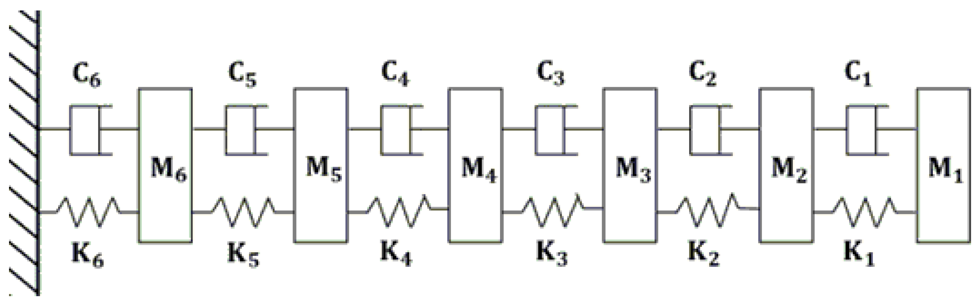
3.1. Six DOF Chain Model of a Cantilever Beam

To illustrate and confirm the validity of the proposed method in this paper, we first consider a numerical example of a chain model with six degrees of freedom (6-DOF) to simulate a cantilever beam, as shown schematically in Figure 1. The masses $m { }_1$, $m { }_2$, $m { }_3$, $m { }_4$, $m { }_5$, and $m { }_6$ for the 6-DOF chain model are equal to 2, 2, 2, 2, 3, and 4 kg. The stiffnesses $k { }_1$, $k{ }_2$, $k { }_3$, $k { }_4$, $k { }_5$, and $k { }_6$ are equal to 1, 1, 1, 1, 2, and 3 N/m, respectively. The damping matrix $\left[C\right]$ of the system is in the form of $\left[C\right]=0.1\left[M\right]+0.001\left[K\right]\raisebox{1ex}{$\mathrm{N}·\mathrm{s}$}\!\left/ \!\raisebox{-1ex}{$\mathrm{m}$}\right.$, which indicates that this structure contains proportional damping because of damping matrix $\left[C\right]$, expressed as the linear combination of the mass matrix $\left[M\right]$ and stiffness matrix $\left[K\right]$. The excitation force is simulated as stationary white noise, which is approximately generated as a zero-mean band-pass noise [21], whose frequency range is from 0 to 50 Hz, and the standard deviation, i.e., power spectrum density, is $0.04 {\mathrm{N}}^2·\mathrm{s}/\mathrm{rad}$. The sampling interval is chosen as $\Delta t=0.01\hspace{0.17em}\mathrm{s}$, and the sampling period, as shown in Figure 2, is $T=N_t·\Delta t=1310.72\hspace{0.17em}\mathrm{s}$, where $N_t$ was chosen as $2^{17}$. The cut-off frequency, ${\omega }_c$ is $314.15 \mathrm{rad}/\mathrm{s}$, and the resolution in frequency domain $\Delta \omega$ is $4{.79 \times 10}^{-3} \mathrm{rad}/\mathrm{s}$. The sampling interval is chosen as 0.01 s, and the sampling period is 150 s. Through Newmark’s method, the displacement responses of the system are obtained and then employed for modal estimation through the modified SSI method.

By introducing the procedure of solving the system matrix in SSI-COV, in conjunction with SSI-DATA, we can increase the computational efficiency without using the original large-dimension data matrix, through the singular value decomposition of the improved projection matrix. To make the number of modes evaluated through the SSI algorithm equal to or greater than the number of modes to be identified, the dimensions of the Hankel matrix must be not less than the system order to be identified ($li\ge 2n$). Through the channel expansion technique, we set the number of expansion channels to 20.

In practical engineering analysis, a continuum structure has an infinite number of degrees of freedom and modes; thus, the dimensions of the Hankel matrix depend on the number of modes to be identified. The projection matrix, $[\Omega ]$ is obtained by Hankel matrix calculation. The SVD analysis of the projection matrix $[\Omega ]$ can then be performed, and the number of singular values is employed to determine the order of system to be identified. In Figure 3 and Figure 4, the distribution of the singular values of $[\Omega ]{[\Omega ]}^T$ shows a relatively more obvious drop than those of $[\Omega ]$ around the singular value number 12 and can be further employed to estimate the system order and the number of modes to be identified. In addition, the SVD analysis of $[\Omega ]{[\Omega ]}^T$ can be employed to reduce a greater number of calculations, rather than performing the SVD of $[\Omega ]$ or system matrix $[A]$. A comparison of the computational efficiency of SVD between $[\Omega ]$ and $[\Omega ]{[\Omega ]}^T$ for different sampling points is shown in

Table 1. Comparison of computation time of SVD of $[\Omega ]$ and $[\Omega ]{[\Omega ]}^T$ for different sampling points as well as matrix multiplication processing time for $[\Omega ]{[\Omega ]}^T$.

Sampling Points	Computation Time (s) of SVD		Matrix Multiplication Processing Time for $[\mathbf{\Omega }]{[\mathbf{\Omega }]}^{\mathit{T}}$
	$[\mathbf{\Omega }]$	$[\mathbf{\Omega }]{[\mathbf{\Omega }]}^{\mathit{T}}$
212	0.570	0.000574	0.0003616
213	2.217	0.000760	0.0005376
214	9.074	0.001219	0.0009967
215	37.197	0.003244	0.0029074
216	Out of memory	0.003264	0.0030135
217	Out of memory	0.006189	0.0059404

Central processing unit (CPU) is Intel^® Core™ i7-9700K CPU @ 3.60 GHz. Random-access memory (RAM) is 64.0 GB.

, in which we clearly see the computation time of SVD of $[\Omega ]$ is much longer than that of $[\Omega ]{[\Omega ]}^T$, especially for $[\Omega ]$ with high dimensions. In addition, through the stabilization diagram of different polynomial orders constructed by identified natural frequency, corresponding to eigenvalues from the frequency response function matrix with different polynomial orders, estimation results can then be sorted as either structural or fictitious modes. In addition, the number of structural modes can clearly be seen to be six, as shown in Figure 5.

In the stabilization diagram, a clear “location” of modal frequency obviously exists, even though no obvious peaks appear among close modes in the frequency response function because of modal interference. The system matrix, $[A]$, can be obtained from Equations (9)–(11), and the modal parameters can then be estimated through the eigenvalue analysis of system matrix, $[A]$, as summarized in

Table 2. Identification results of 6-DOF chain model through Modified Stochastic Subspace Identification (MSSI) method from projection matrix $[\Omega ]$.

Mode	Natural Frequency (rad/s)			Damping Ratio (%)
	Exact	MSSI	Error (%)	Exact	MSSI	Error (%)
1	5.03	5.04	0.09	1.25	1.38	10.39
2	13.45	13.39	0.41	1.04	1.17	11.73
3	19.80	19.71	0.41	1.24	1.23	0.92
4	26.68	26.56	0.44	1.52	1.47	3.59
5	31.65	31.18	1.48	1.74	1.79	2.78
6	33.72	33.46	0.78	1.84	1.89	3.18

and

Table 3. Identification results of 6-DOF chain model through Modified Stochastic Subspace Identification (MSSI) method from the data matrix $[\Omega ]{[\Omega ]}^T$ constructed by projection matrix.

Mode	Natural Frequency (rad/s)			Damping Ratio (%)
	Exact	MSSI	Error (%)	Exact	MSSI	Error (%)
1	5.03	5.04	0.08	1.25	1.38	8.97
2	13.45	13.39	0.42	1.04	1.17	10.11
3	19.80	19.71	0.42	1.24	1.23	2.47
4	26.68	26.56	0.47	1.52	1.47	4.88
5	31.65	31.18	1.50	1.74	1.79	1.15
6	33.72	33.46	0.78	1.84	1.89	1.19

, where we clearly see the well-estimated structural modal parameters through the Modified Stochastic Subspace Identification (MSSI) method of both $[\Omega ]$ and $[\Omega ]{[\Omega ]}^T$. Note that the MSSI method is a combination of the conventional SSI method and SVD analysis. A comparison between the exact and identified mode shapes is shown in Figure 6, and the corresponding Modal Assurance Criterion (MAC) [22] values evaluated are shown in Figure 7, where good agreement is observed.

3.2. Six DOF Railway Vehicle Model with Modal Interference

In the previous examples, only a proportionally damped structure is considered. Actually, the hypothesis of proportional damping, although frequently considered in the literature, is difficult to be found in practice in real mechanical systems [23,24]. To study the feasibility and validity of the proposed method for relatively complex structural systems, we consider a linear 6-DOF railway vehicle model with viscous damping [25], as shown schematically in Figure 8. The mass matrix $M$, stiffness matrix $K$, and the damping matrix $C$ of the system are given as follows [26]:

$$M=\left[\begin{array}{cccccc}1200& 0& 0& 0& 0& 0\\ 0& 850& 0& 0& 0& 0\\ 0& 0& 4125& 0& 0& 0\\ 0& 0& 0& 125000& 0& 0\\ 0& 0& 0& 0& 850& 0\\ 0& 0& 0& 0& 0& 1220\end{array}\right]\mathrm{kg}$$

$$K=\left[\begin{array}{cccccc}{k}_1+k_2& {-k}_2& 0& 0& 0& 0\\ {-k}_2& k_2+k_3& {-k}_3& {-k}_{3}L& 0& 0\\ 0& {-k}_3& k_3+k_4& k_{3}L-k_{4}L& -k_4& 0\\ 0& {-k}_{3}L& k_{3}L-k_{4}L& k_3{L}^2+k_4{L}^2& k_{4}L& 0\\ 0& 0& -k_4& k_{4}L& k_4+k_5& {-k}_5\\ 0& 0& 0& 0& {-k}_5& k_5+k_6\end{array}\right]\mathrm{N}/\mathrm{m}$$

$$C=\left[\begin{array}{cccccc}{c}_1+c_2& {-c}_2& 0& 0& 0& 0\\ {-c}_2& c_2+c_3& {-c}_3& {-c}_{3}L& 0& 0\\ 0& {-c}_3& c_3+c_4& c_{3}L-c_{4}L& -c_4& 0\\ 0& {-c}_{3}L& c_{3}L-c_{4}L& c_3{L}^2+c_4{L}^2& c_{4}L& 0\\ 0& 0& -k_4& c_{4}L& c_4+c_5& {-c}_5\\ 0& 0& 0& 0& {-c}_5& c_5+c_6\end{array}\right]\raisebox{1ex}{$\mathrm{N}·\mathrm{s}$}\!\left/ \!\raisebox{-1ex}{$\mathrm{m}$}\right.$$

in which $K_1=3\times {10}^7 \mathrm{N}/\mathrm{m}$, $K_2={10}^6 \mathrm{N}/\mathrm{m}$, $K_3=6\times {10}^6 \mathrm{N}/\mathrm{m}$, $K_4=6\times {10}^6 \mathrm{N}/\mathrm{m}$, $K_5={10}^6 \mathrm{N}/\mathrm{m}$, $K_6=3\times {10}^7 \mathrm{N}/\mathrm{m}$, L = 8.53 m, $c_1=0$, $c_2=6\times {10}^3 \mathrm{N}·\mathrm{s}/\mathrm{m}$, $c_3=1.8\times {10}^4 \mathrm{N}·\mathrm{s}/\mathrm{m}$, $c_4=1.8\times {10}^4 \mathrm{N}·\mathrm{s}/\mathrm{m}$, $c_5=6\times {10}^3 \mathrm{N}·\mathrm{s}/\mathrm{m}$, and $c_6=0$. This railway structural system has the features of relatively high modal damping levels for third and fourth modes, and a pair of closely spaced fifth and sixth modes. Note that this railway structure has non-proportional damping, because damping matrix, $C$, cannot be expressed as the linear combination of the mass matrix, $M$, and stiffness matrix, $K$. The stationary white noise in the previous numerical example is still used as the excitation force acting the 6th mass of the railway vehicle system. The sampling interval is set as 0.01 s, and the sampling period is 110 s. Then, using Newmark’s method, the displacement responses obtained are employed for modal estimation using the modified SSI method proposed in this paper.

It should be noted that the number of modes to be identified serves to determine the dimensions of the Hankel matrix. Using the channel expansion technique, we set the number of expansion channels at 20. The dimensions of the Hankel matrix are not less than the order of the system to be identified, thus satisfying the condition that the number of modes evaluated in the SSI algorithm is not less than the number of modes to be identified. The SVD analysis of the projection matrix, which is obtained from the Hankel matrix calculation, can then be implemented, and the number of singular values is employed to determine the order of the system to be identified. Around the 12th singular value, an obvious drop showed in the distribution of singular values associated with the data matrix $[\Omega ]{[\Omega ]}^T$ constructed by projection matrix $[\Omega ]$ from stationary response data, as shown in Figure 9. It can be estimated that the order of the system, i.e., the number of modes to be identified, is 12.

Compared with the efficiency when performing the SVD of the system matrix $[A]$, computation can be reduced by implementing SVD analysis of data matrix $[\Omega ]{[\Omega ]}^T$ constructed from the projection matrix $[\Omega ]$. As shown in Figure 10, from the stabilization diagram corresponding to different modal orders, it can be observed that the number of structural modes to be identified is six, and serious modal interference can be observed between the last two close modes. The system matrix, $[A]$, can be found using Equations (9)–(11), and the modal parameters can then be determined through Equations (12)–(15).

Table 4. Identification results of railway vehicle through Modified Stochastic Subspace Identification (MSSI) method.

Mode	Natural Frequency (Hz)			Damping Ratio (%)
	Exact	MSSI	Error (%)	Exact	MSSI	Error (%)
1	2.79	2.79	0.00	4.89	4.89	0.01
2	3.71	3.71	0.00	6.62	6.62	0.01
3	16.55	16.53	0.09	16.65	16.62	0.17
4	19.27	19.25	0.11	18.78	18.74	0.24
5	25.36	25.30	0.21	1.74	1.74	0.42
6	25.57	25.51	0.21	1.75	1.75	0.43

presents the well-implemented modal estimation through eigenvalue analysis of the system matrix, $[A]$. A comparison between the exact and identified mode shapes is shown in Figure 11, and the corresponding MAC values evaluated are shown in Figure 12, where good agreement is observed.

Due to the experimental restrictions of economic cost and structural geometry in the practical measurement of structural response, the number of sensors sited on the structures to record response data is not usually sufficient for the overall degrees of freedom of a structure to be identified. This may cause problems of incomplete measurement of the degrees of freedom of the identified mode-shape vector. To address this issue, we also implement modal estimation from the incomplete modal-information data obtained due to insufficient measurement channels; thus, only response data of the first, third, and fifth DOF of the railway system subjected to ambient excitation in the previous numerical example are employed to implement modal estimation. The modal estimation results are shown in

Table 5. Identification results of railway vehicle through Modified Stochastic Subspace Identification (MSSI) method from incomplete modal-information measurement data.

Mode	Natural Frequency (rad/s) $[\mathbf{\Omega }]$			Damping Ratio (%)
	Exact	MSSI	Error (%)	Exact	MSSI	Error (%)
1	2.79	2.79	0.00	4.89	4.89	0.01
2	3.71	3.71	0.00	6.62	6.62	0.01
3	16.55	16.53	0.09	16.65	16.62	0.16
4	19.27	19.25	0.12	18.78	18.73	0.27
5	25.36	25.30	0.21	1.74	1.74	0.42
6	25.57	25.51	0.21	1.75	1.75	0.42

. The modal parameters estimated by the proposed method and the exact results are in good agreement, because the errors in both natural frequencies and damping ratios are less than 1%. Thus, we confirm the effectiveness of the proposed method under the likely practical conditions of insufficient measurement information.

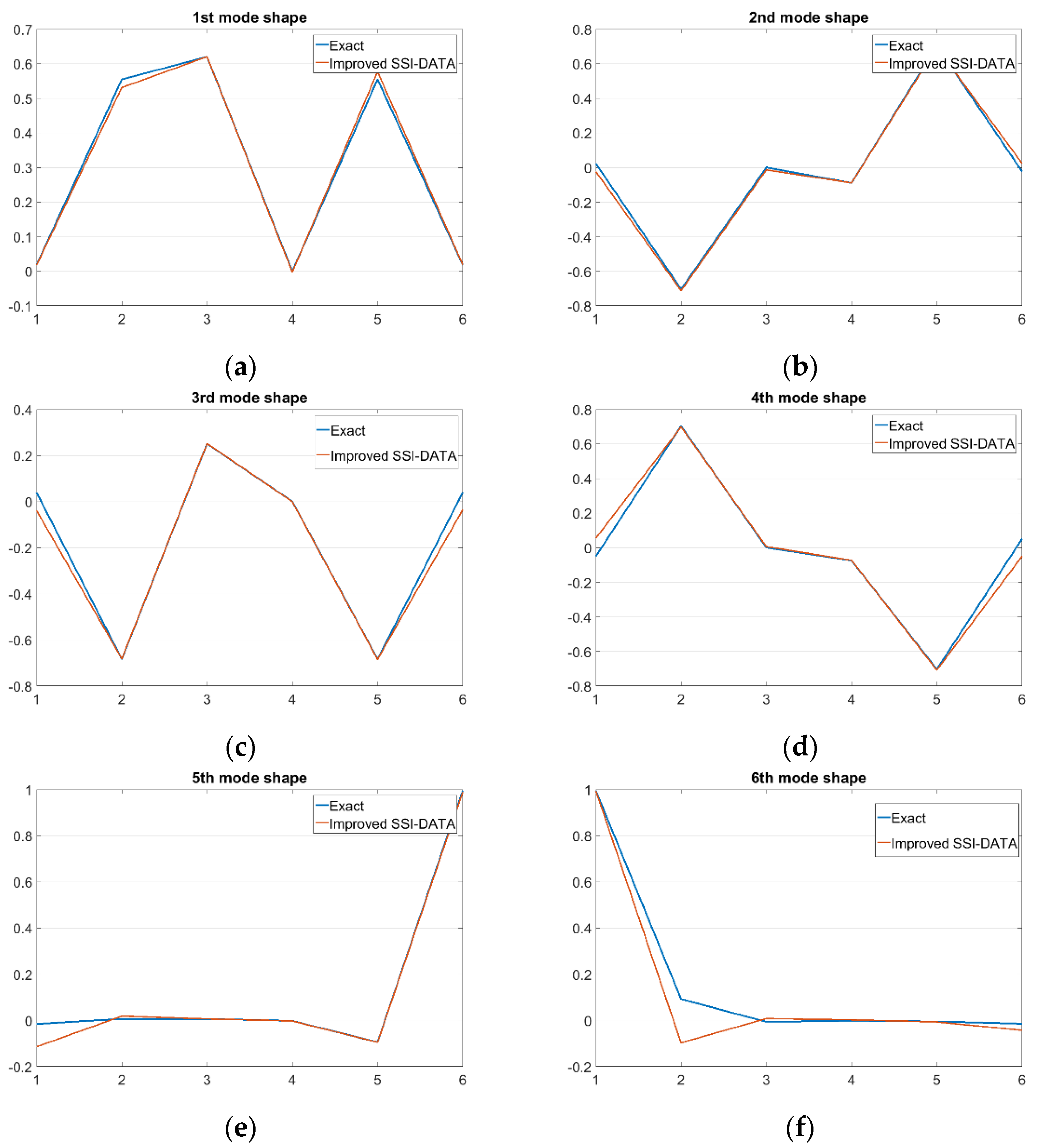
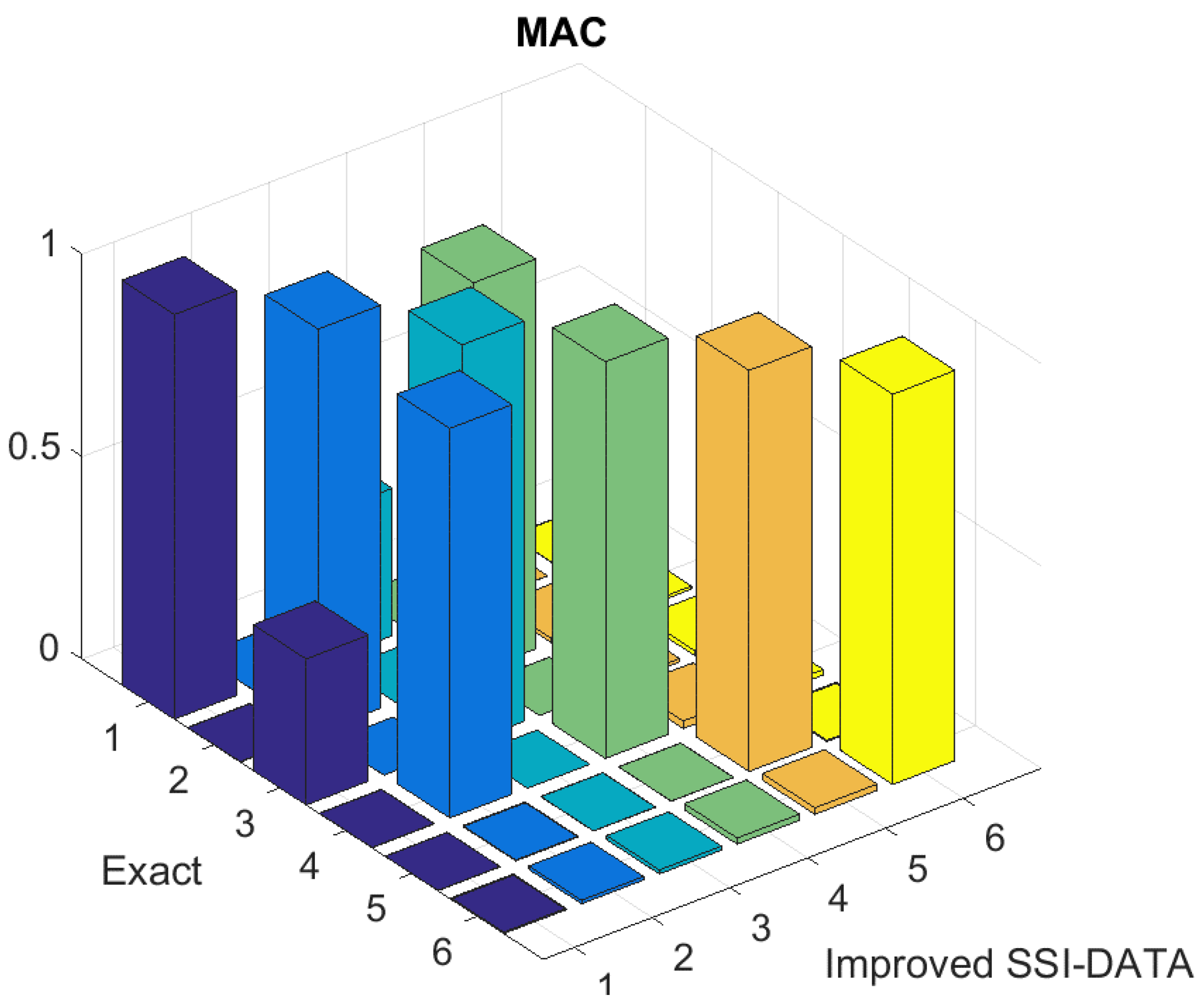
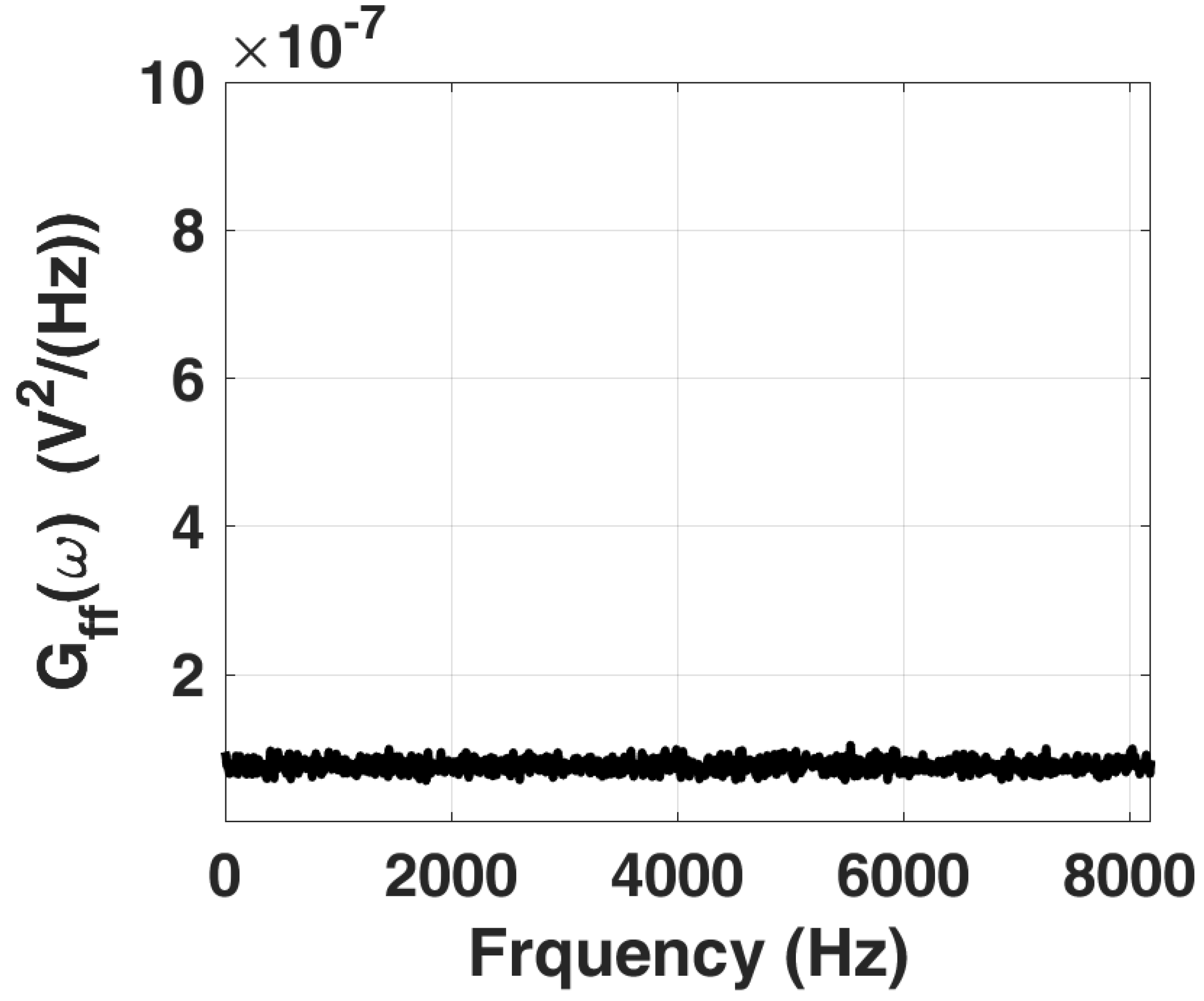
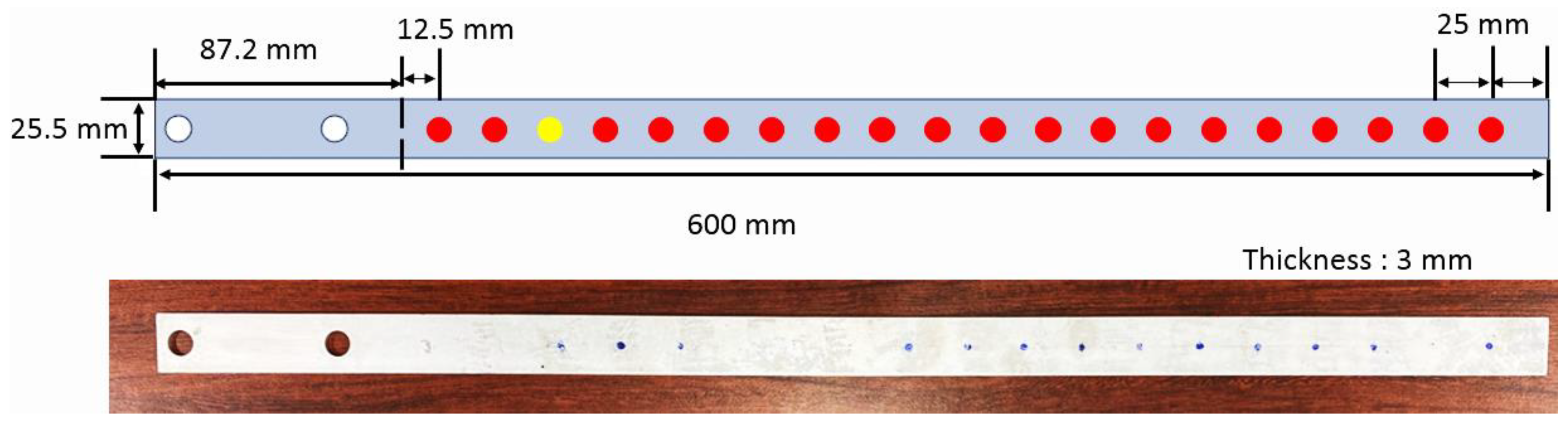
3.3. Experimental Validation of a Cantilever Beam

To further validate the effectiveness of the method proposed in this paper, an actual beam structure of free boundary is used for the experiment, as shown in Figure 13. Brüel & Kjær RT Pro Photon 7.41 data acquisition system, PCB 208C02 force sensor (with a sensitivity of 112,410 mV/kN, a measurement range of 0.4448 kN, a low frequency response (−5%) of 0.001 Hz, and an upper frequency limit of 36,000 Hz), and Polytec OFV-5000 Modular Vibrometer (having a frequency range of DC-24 MHz with velocities up to ±10 m/s and displacements from the picometer to meter range) are used for measuring response signal. The simulated nonstationary excitation through Teledyne LeCroy T3AFG40 signal generator is imported into the Modal Shop K20070E01 vibration exciter, and the vibration shaker excites the cantilever beam structure. A typical white noise with an approximately consistent-power spectral density was synchronized with the shaker voltage time history and recorded, as shown in Figure 14, as provided from the waveform source panel in the RT Pro Photon 7.41 data acquisition system. Currently, an OMA-based roving different directions of sensor head of laser doppler vibrometer is performed to measure the actual modal properties of the beam structure by the data acquisition device, including four channels, only twenty measurement positions on the actual aluminum alloy beam were marked, as shown in Figure 15, and the shaker excitation impacts acted as the third location of the beam.

The length, width, and height of the beam structure used for this paper are 512.8, 25.5, and 3.0 mm, respectively, the mass is 104.97 g, and the material is 5052-0 aluminum alloy. In addition, the “exact” modal parameters are obtained from the data of auto power spectrum of stationary response and cross power spectrum of stationary excitation and response by using ME’Scope software. Note that “exact” stationary excitation is a built-in stationary white noise generated from Brüel & Kjær RT Pro Photon 7.41 data acquisition system is imported into the Modal Shop K20070E01 electrodynamic shaker to excite the cantilever beam structure. The natural frequencies of the first four modes are about 10.85, 70.32, 176.31, and 290.31 Hz, as listed in

Table 6. Identification results of a practical cantilever beam through Modified Stochastic Subspace Identification (MSSI) method.

Mode	Natural Frequency (rad/s)			MAC
	Exact	MSSI	Error (%)
1	10.85	10.98	1.22	1.00
2	70.32	70.53	0.30	1.00
3	176.31	159.00	9.82	0.95
4	290.31	246.30	15.16	0.77

. Finally, the modal parameters obtained are used to compare the identification results of MSSI, as shown in Table 6 and Figure 16. It is observed that the frequency errors are less than 15%, Figure 16 shows the identified mode shapes which are approximately coincident with “exact” mode shapes, and the MAC values are larger than 0.77. This means that the proposed method is effective on modal identification in practical application.

4. Conclusions

The topic of this paper was a study of ambient modal analysis based on the stochastic subspace identification technique (SSI). The paper aimed to develop the appropriate algorithms for output-only modal analysis to overcome difficulties when performing experimental modal analysis (EMA). As a modification of SSI, we introduced the procedure of solving the system matrix in SSI-COV in conjunction with SSI-DATA, allowing modal estimation to be well implemented. A system matrix can, therefore, be obtained directly from the observability matrix without evaluating the predictive-state matrix, and this will improve the efficiency of computation.

In addition, we extracted predictive-state matrixes with recursive relationships directly from the same original predictive-state matrix, and then omitted the step of reevaluating the predictive-state matrix at the next-time moment to improve the computational efficiency of the SSI method. In addition, through the SVD analysis of a data matrix $[\Omega ]{[\Omega ]}^T$, evaluated by the projection matrix, $[\Omega ]$, the modal estimation can be effectively performed, and the corresponding computational efficiency can be improved.

By solving the system matrix through the observability matrix and constructing a new predictive-state matrix composed from the original measured data matrix, the procedure of modal estimation can be simplified, and the modal parameters can be effectively identified, even for a structural system having closely spaced modes and relatively high damping. Furthermore, the proposed modified SSI algorithm is applicable to the parametric estimation of structures with incomplete modal information obtained from insufficient measurement channels. In addition, the computational efficiency of the SSI method can be improved due to the non-uniqueness of the observability matrix. However, the need for white noise excitation is still a main limitation to be resolved in the proposed method from ambient response, and many mechanical systems are expected to be excited by significantly different frequency content, in particular, by specific harmonics [27,28]. The actual limitations and the applicability of the proposed method to real mechanical systems could be considered for discussion in future work. Through numerical simulations and experimental verification, we illustrated and validated the effectiveness of the proposed method for modal estimation of structural systems from stationary ambient response data only.

References

1. Martini, A.; Troncossi, M.; Vincenzi, N. Structural and elastodynamic analysis of rotary transfer machines by Finite Element model. J. Serb. Soc. Comput. Mech. 2017, 11, 1–16. [Google Scholar] [CrossRef] [Green Version]
2. Manzato, S.; Peeters, B. Wind turbine model validation by full-scale vibration test. In Proceedings of the European Wind Energy Conference (EWEC) 2010, Warsaw, Poland, 20–23 April 2010. [Google Scholar]
3. Zivanovic, S.; Pavic, A.; Reynolds, P. Modal Testing and FE Model Tuning of a Lively Footbridge Structure. Eng. Struct. 2006, 28, 857–868. [Google Scholar] [CrossRef] [Green Version]
4. Ren, W.X.; Peng, X.L.; Lin, Y.Q. Experimental and Analytical Studies on Dynamic Characteristics of a large Span Cables-stayed Bridge. Eng. Struct. 2005, 27, 535–548. [Google Scholar] [CrossRef]
5. Orlowitz, E.; Brandt, A. Comparison of experimental and operational modal analysis on a laboratory test plate. Measurement 2007, 102, 121–130. [Google Scholar] [CrossRef]
6. Moaveni, B.; Masoumi, Z. Modifying the ERA and fast ERA to improve operational performance for structural system identification. Mech. Syst. Signal Process. 2019, 120, 664–692. [Google Scholar] [CrossRef]
7. Brincker, R.; Kirkegaard, P.H. Special issue on Operational Modal Analysis. Mech. Syst. Signal Process. 2010, 24, 1209–1212. [Google Scholar] [CrossRef]
8. Reynders, E.; Houbrechts, J.; De Roeck, G. Fully automated (operational) modal analysis. Mech. Syst. Signal Process. 2012, 29, 228–250. [Google Scholar] [CrossRef]
9. Yi, W.J.; Zhou, Y.; Kunnath, S.; Xu, B. Identification of localized frame parameters using higher natural modes. Eng. Struct. 2008, 30, 3082–3094. [Google Scholar] [CrossRef]
10. Soria, L.; Peeters, B.; Anthonis, J. Operational modal analysis and the performance assessment of vehicle suspension systems. Shock. Vib. 2012, 19, 1099–1113. [Google Scholar] [CrossRef]
11. Shirzadeh, R.; Devriendt, C.; Bidakhvidi, M.A.; Guillaume, P. Experimental and computational damping estimation of an offshore wind turbine on a monopile foundation. J. Wind. Eng. Ind. Aerodyn. 2013, 120, 96–106. [Google Scholar] [CrossRef]
12. Peeters, B.; Van der Auweraer, H.; Vanhollebeke, F.; Guillaume, P. Operational modal analysis for estimating the dynamic properties of a stadium structure during a football game. Shock. Vib. 2007, 14, 283–303. [Google Scholar] [CrossRef]
13. James, G.H.; Carne, T.G.; Lauffer, J.P. The Natural Excitation Technique for Modal Parameter Extraction from Operating Wind Turbines; SAND92-1666.UC-261; Sandia National Laboratories: Albuquerque, NM, USA, 1993.
14. Chiang, D.-Y.; Lin, C.-S. Identification of Modal Parameters from Nonstationary Ambient Vibration Data Using Correlation Technique. AIAA J. 2008, 46, 2752–2759. [Google Scholar] [CrossRef]
15. Lin, C.-S.; Chiang, D.-Y. Modal identification from nonstationary ambient response data using extended random decrement algorithm. Comput. Struct. 2013, 119, 104–114. [Google Scholar] [CrossRef]
16. Chiang, D.-Y.; Lin, C.-S. Identification of modal parameters from ambient vibration data using eigensystem realization algorithm with correlation technique. J. Mech. Sci. Technol. 2010, 24, 2377–2382. [Google Scholar] [CrossRef]
17. Liu, F.; Wu, J.; Gu, F.; Ball, A.D. An Introduction of a Robust OMA Method: CoS-SSI and Its Performance Evaluation through the Simulation and a Case Study. Shock. Vib. 2019, 2019, 1–14. [Google Scholar] [CrossRef]
18. Van Overschee, P.; De Moor, B. Subspace algorithms for the stochastic identification problem. Automatica 1993, 29, 649–660. [Google Scholar] [CrossRef]
19. Shokravi, H.; Shokravi, H.; Bakhary, N.; Koloor, S.S.R.; Petrů, M. Health Monitoring of Civil Infrastructures by Subspace System Identification Method: An Overview. Appl. Sci. 2020, 10, 2786. [Google Scholar] [CrossRef] [Green Version]
20. Peeters, B.; De Roeck, G. Reference-based stochastic subspace identification for output-only modal analysis. Mech. Syst. Signal Process. 1999, 13, 855–878. [Google Scholar] [CrossRef] [Green Version]
21. Shinozuka, M. Simulation of Multivariate and Multidimensional Random Processes. J. Acoust. Soc. Am. 1971, 49, 357–368. [Google Scholar] [CrossRef]
22. Allemang, R.J. The Modal Assurance Criterion—Twenty Years of Use and Abuse. Sound Vib. 2003, 37, 14–23. [Google Scholar]
23. Troncossi, M.; Taddia, S.; Rivola, A.; Martini, A. Experimental Characterization of a High-Damping Viscoelastic Material Enclosed in Carbon Fiber Reinforced Polymer Components. Appl. Sci. 2020, 10, 6193. [Google Scholar] [CrossRef]
24. Troncossi, M.; Canella, G.; Vincenzi, N. Identification of polymer concrete damping properties. Proc. Inst. Mech. Eng. Part C J. Mech. Eng. Sci. 2020, in press. [Google Scholar] [CrossRef]
25. Petsounis, K.; Fassois, S. Parametric time-domain methods for the identification of vibrating structures—A critical comparison and assessment. Mech. Syst. Signal Process. 2001, 15, 1031–1060. [Google Scholar] [CrossRef]
26. Hu, S.-L.J.; Yang, W.-L.; Liu, F.-S.; Li, H.-J. Fundamental comparison of time-domain experimental modal analysis methods based on high- and first-order matrix models. J. Sound Vib. 2014, 333, 6869–6884. [Google Scholar] [CrossRef]
27. Campione, I.; Fragassa, C.; Martini, A. Kinematics optimization of the polishing process of large-sized ceramic slabs. Int. J. Adv. Manuf. Technol. 2019, 103, 1325–1336. [Google Scholar] [CrossRef]
28. Zaghbani, I.; Songmene, V. Estimation of machine-tool dynamic parameters during machining operation through operational modal analysis. Int. J. Mach. Tools Manuf. 2009, 49, 947–957. [Google Scholar] [CrossRef]
Figure 1. Schematic plot of a 6-DOF chain model of a cantilever beam.
Applsci 11 11751 g001
Figure 2. A sample function of stationary white noise in the time domain.
Applsci 11 11751 g002
Figure 3. Distribution of the singular values of projection matrix [ Ω ] from the stationary responses of a 6-DOF chain model of a cantilever beam.
Applsci 11 11751 g003
Figure 4. Distribution of the singular values of the data matrix, [ Ω ] [ Ω ] T , constructed by projection matrix, [ Ω ] , from the stationary responses of a 6-DOF chain model of a cantilever beam.
Applsci 11 11751 g004
Figure 5. Typical plot of the stabilization diagram of stationary response of first DOF of a 6-DOF chain model of a cantilever beam.
Applsci 11 11751 g005
Figure 6. Comparison between the identified mode shapes and the exact mode shapes of a 6-DOF chain model of a cantilever beam subjected to stationary white noise: (a) 1st bending mode shape; (b) 2nd bending mode shape; (c) 3rd bending mode shape; (d) 4th bending mode shape; (e) 5th bending mode shape; (f) 6th bending mode shape.
Applsci 11 11751 g006aApplsci 11 11751 g006b
Figure 7. Typical plot of the Modal Assurance Criterion (MAC) for the identified mode shapes and exact mode shapes of a 6-DOF chain model of a cantilever beam.
Applsci 11 11751 g007
Figure 8. Schematic plot of the railway vehicle model.
Applsci 11 11751 g008
Figure 9. Distribution of the singular values associated with a data matrix, [ Ω ] [ Ω ] T , constructed by projection matrix, [ Ω ] , from stationary responses of a railway vehicle model..
Applsci 11 11751 g009
Figure 10. Typical plot of the stabilization diagram of stationary responses of 1st DOF of a 6-DOF chain model of a railway vehicle.
Applsci 11 11751 g010
Figure 11. Comparison between the identified mode shapes and the exact mode shapes of 6-DOF chain model of a railway vehicle subjected to stationary white noise: (a) 1st mode shape; (b) 2nd mode shape; (c) 3rd mode shape; (d) 4th mode shape; (e) 5th mode shape; (f) 6th mode shape.
Applsci 11 11751 g011
Figure 12. Typical plot of the Modal Assurance Criterion (MAC) for the identified mode shapes and exact mode shapes of 6-DOF chain model of a railway vehicle.
Applsci 11 11751 g012
Figure 13. Schematic diagram of the experimental setup.
Applsci 11 11751 g013
Figure 14. Power spectrum associated with stationary white noise.
Applsci 11 11751 g014
Figure 15. Twenty measurement positions marked on the actual aluminum alloy beam.
Applsci 11 11751 g015
Figure 16. Comparison between the identified mode shapes and the “exact” mode shapes of a practical cantilever beam subjected to stationary white noise: (a) 1st mode shape; (b) 2nd mode shape; (c) 3rd mode shape; (d) 4th mode shape.
Applsci 11 11751 g016