Article

Continuous Emotion Recognition with Spatiotemporal Convolutional Neural Networks

by
Thomas Teixeira
,
Éric Granger
and
Alessandro Lameiras Koerich
*
École de Technologie Supérieure, Université du Québec, 1100, Rue Notre-Dame Ouest, Montreal, QC H3C 1K3, Canada
*
Author to whom correspondence should be addressed.
Appl. Sci. 2021, 11(24), 11738; https://doi.org/10.3390/app112411738
Submission received: 4 November 2021 / Revised: 8 December 2021 / Accepted: 8 December 2021 / Published: 10 December 2021
(This article belongs to the Special Issue Research on Facial Expression Recognition)

Abstract

:
Facial expressions are one of the most powerful ways to depict specific patterns in human behavior and describe the human emotional state. However, despite the impressive advances of affective computing over the last decade, automatic video-based systems for facial expression recognition still cannot correctly handle variations in facial expression among individuals as well as cross-cultural and demographic aspects. Nevertheless, recognizing facial expressions is a difficult task, even for humans. This paper investigates the suitability of state-of-the-art deep learning architectures based on convolutional neural networks (CNNs) to deal with long video sequences captured in the wild for continuous emotion recognition. For such an aim, several 2D CNN models that were designed to model spatial information are extended to allow spatiotemporal representation learning from videos, considering a complex and multi-dimensional emotion space, where continuous values of valence and arousal must be predicted. We have developed and evaluated convolutional recurrent neural networks, combining 2D CNNs and long short term-memory units and inflated 3D CNN models, which are built by inflating the weights of a pre-trained 2D CNN model during fine-tuning, using application-specific videos. Experimental results on the challenging SEWA-DB dataset have shown that these architectures can effectively be fine-tuned to encode spatiotemporal information from successive raw pixel images and achieve state-of-the-art results on such a dataset.

1. Introduction

Facial expressions are the results of peculiar positions and movements of facial muscles over time. According to previous studies, face images and videos provide an essential source of information for representing the emotional state of an individual [1]. Therefore, facial expression recognition (FER) has attracted a growing interest in recent years. However, the detection of spontaneous facial expressions in the wild is a very challenging task. The performance depends on several factors, such as variations among individuals, the identity bias of subjects (e.g., gender, age, culture, and ethnicity), and the quality of recordings (e.g., illumination, resolution, head pose, and capture conditions).
The fundamentals of human affect theory [2,3] inspired early research on FER systems. Even if facial expressions can also be performed voluntarily, without any relationship to the emotions that a person actually feels [4,5], FER systems assume that facial expressions are associated with either discrete or multidimensional emotion models. Discrete models are employed to classify facial images into discrete categories that can be recognizable across cultures, such as anger, disgust, fear, happiness, sadness, and surprise. The limited generalization capacity of these models has paved the way for multidimensional spaces that can improve the representativeness and accuracy for describing emotions [6].
There are three levels for describing emotion: pleasantness, attention, and activation. Specifically, emotion recognition datasets annotate emotional states with two values named valence and arousal. The former represents the level of pleasantness, and the latter represents the level of activation, each of these values lying in the [ 1 ; 1 ] range. These values can be used to project an individual emotional state into a 2D space called the circumplex model, which is shown in Figure 1. The level of arousal is represented on the vertical axis, whereas the valence level is represented on the horizontal axis.
Early FER systems relied on shallow approaches, which combined handcrafted features, such as eigenfaces [8], Gabor wavelets [9], local binary patterns (LBP) [10,11] and its variants (such as LBP-TOP [12] and LBP-SIP [13]), and Weber local descriptor [14] with support vector machines (SVM). However, recent advances in deep learning (DL) and computing technologies have led FER systems to learn discriminant representations directly from face images. Previous studies first exploited static FER datasets, where subjects are associated with discrete and mutually exclusive categories of emotions. State-of-the-art performance on benchmarking datasets, such as FER2013 [15], TFD [16], and SFEW [17], was achieved using CNN-based approaches [18,19,20,21,22,23,24].
Temporal information and dynamic facial components can play a crucial role in describing facial expressions [1]. By definition, people express emotions in a dynamic process, and learning spatiotemporal structures has become the current trend. Recent studies have proposed deep architectures for FER, which were trained on video data [25]. In the literature, video sequences are mostly processed using aggregation and concatenation of features for each facial image into clips. Yet, they cannot leverage the temporal dependencies over a video [26,27]. To circumvent this issue, convolutional recurrent neural networks (CRNN) and 3D-CNN architectures have been proposed to encode spatiotemporal relations among video frames [28,29].
This paper investigates and compares state-of-the-art DL models based on CNNs for video-based emotion recognition, where affective states are represented as continuous values in the bidimensional space of valence and arousal. The novelty of this paper is the extension of state-of-the-art 2D CNN architectures to model spatiotemporal relations of facial features in videos with the aim of improving the predictions for continuous values of emotion. Starting from pre-trained 2D CNNs, two types of DL models are fine-tuned with videos: (i) a 2D CNN combined with a long short-term memory (LSTM) structure; and (ii) a 2D CNN inflated into a 3D CNN. These models predict emotions through regression of valence and arousal values. Long video sequences are captured in the wild and split into several clips to augment training data and isolate unique facial expressions. For proof-of-concept, CNN architectures, such as VGG and ResNet, were pre-trained with ImageNet and RAF-DB datasets and fine-tuned with multiple video sequences from the SEWA-DB dataset to predict continuous values of valence and arousal. Experiments were conducted over different clip lengths, overlapping ratios, and strategies for fusing annotations.
The main contributions of this paper are (i) spatiotemporal models, combining pre-trained 2D CNNs and LSTM units for continuous emotion recognition that achieve state-of-the-art performance on SEWA-DB; (ii) a comparative study on the impact of the dataset used for pre-training and level of fine-tuning on the accuracy of different CNN models for discrete emotion recognition; and (iii) a novel spatiotemporal model based on an inflated pre-trained 2D CNN for continuous emotion recognition.
This paper is organized as follows. Section 2 provides a review of DL models proposed for emotion recognition in videos captured in the wild, focusing on models that allow encoding the spatiotemporal relations in facial emotions. Section 3 presents an overview of DL models that are proposed for continuous emotion recognition, including pre-processing steps, model architectures, pre-training, fine-tuning procedures, and post-processing steps. Section 4 describes the experimental methodology (e.g., protocol, datasets and performance metrics) used to validate DL models for continuous emotion recognition, as well as the experimental results. Section 5 presents a discussion and a comparison with the state of the art. Conclusions are presented in the last section.

2. Related Works

A conventional approach for dealing with video frames is to aggregate features extracted from each frame into a clip before final emotion prediction Ding et al. [27]. In addition to feature aggregation, Bargal et al. [26] also aggregated the mean, variance, minimum and maximum over a sequence of features, thus adding some statistical information. However, since feature aggregation cannot exploit inter-correlations between frames and cannot depict temporal dependencies, this approach has substantial limitations. To circumvent this issue, recurrent neural networks (RNN), such as LSTM or 3D CNN architectures, can integrate data series as input, provided that data are sequentially ordered, and transitions have a substantial potential for information. While LSTMs can deal with sequential data of variable length in both directions, 3D CNNs exploit textured variations from a sequence of images by extending convolutional kernels to a third dimension. Hence, 3D CNNs are well suited to encode spatiotemporal information in video-based FER applications. For example, Tran et al. [30] proposed a 3D CNN model for action recognition on the UCF101 dataset, which encompasses videos classified over 101 action categories. They showed that 3D CNNs can outperform 2D CNNs on different video analysis benchmarks and bring efficient and compact features. Several recent studies [31,32,33,34,35,36,37] proposed approaches based on 3D CNNs for FER. Nevertheless, all of them deal with discrete emotion prediction.
A popular approach for dealing with temporal sequences of frames is a cascaded network in which architectures for representation learning and discrimination are stacked on top of each other. Thus, various levels of features are learned by each block and processed by the following until the final prediction. Notably, the combination of CNNs and LSTM units has been shown to be effective in learning spatiotemporal representations [30,38]. For instance, Ouyang et al. [37] used a VGG-16 CNN to extract a 16-frame sequence of features and fed an LSTM unit to predict six emotion categories. They preprocessed video frames with a multi-task cascade CNN (MTCNN) to detect faces and described each video by a single 16-frame window. Similarly, Vielzeuf et al. [39] used a VGG-16 CNN and an LSTM unit as part of an ensemble with a 3D-CNN and an audio network. Mainly, they used the multi-instance learning (MIL) method to create bag-of-windows for each video with a specific overlapping ratio. Each sequence was described by a single label and contributed to the overall prediction of the matching video clip.
Since deep neural networks (DNNs) are highly data-dependent, there are strong limitations for designing FER systems based on DNNs, even more since FER datasets are often small and task-oriented [1]. Considering this fact, training deep models on FER datasets usually leads to overfitting. In other words, end-to-end training is not feasible if one may learn representation and a discriminant with deep architectures on images with little pre-processing. In this way, some previous works showed that additional task-oriented data for pre-training networks or fine-tuning on well-known pre-trained models could greatly help in building better FER models [40,41]. Pre-training deep neural networks is then essential for not leading DL models to overfit. In this way, several state-of-the-art models were developed and shared for research purposes. For example, VGG-Face [42] is a CNN based on the VGG-16 architecture Simonyan and Zisserman [43] to circumvent the lack of data by building an architecture for face identification and verification and make it available for the research community. This CNN trained on about three million images of 2600 subjects makes this architecture especially adapted for face and emotion recognition. Recent works that have performed well in FER challenges, such as EmotiW [44] or AVEC [45], are based on VGG-Face architecture. Wan et al. [46] combined linear discriminant analysis and weighted principal component analysis with VGG-Face for feature extraction and dimension reduction in a face recognition task. Knyazev et al. [47], as part of the EmotiW challenge, fine-tuned a VGG-Face on the FER2013 dataset [15] and aggregated frame features for classifying emotions on video sequences with a linear SVM. Finally, Ding et al. [48] proposed peculiar fine-tuning techniques with VGG-Face. They constrained their network to act like a VGG-Face network by transferring outputs from late layers rather than transferring weights.
Recent works used 3D convolutional kernels for a spatiotemporal description of visual information. The first 3D-CNN models were developed for the action recognition task [30,34,38]. Three-dimensional CNNs pre-trained on action recognition datasets were then made available and transferred to affect computing research [32,33]. Ouyang et al. [37] combined VGG-Face and LSTM, among other CNN-RNN and 3D CNN networks, to build an ensemble network for multi-modality fusion (video+audio), which predicts seven categories of emotions. We believe no 3D CNN model has been evaluated so far for predicting continuous emotions, and only a few approaches have been proposed for discrete emotion prediction. This is mainly due to the lack of video datasets for FER, which allow exploiting the temporal dimension. To circumvent this issue, Carreira and Zisserman [49] developed the i3D network, which can learn 3D feature representations based on 2D datasets. They inflated a 2D inception CNN to extend learned weights in 2D to a third dimension. In this way, they developed several pre-trained networks based on the same architecture with a combination of ImageNet and Kinetics datasets on images or optical flow inputs. As demonstrated by Carneiro de Melo et al. [29], 3D CNNs for emotion recognition and depression detection [32,33,37] have a lower capacity to produce discriminant spatiotemporal features than i3D [49]. This is mainly because the i3D-CNN is deeper and benefits from efficient neural connections through the inception module. In this way, with inflated 2D networks, efficient 3D CNNs can be built from competitive 2D architectures. Carneiro de Melo et al. [29] proposed a deep maximization-differentiation network (MDN) and compared this architecture with i3D-CNN and T-3D CNN [50], showing that i3D requires fewer parameters than other models and is computationally faster. Finally, Praveen et al. [51,52] applied i3D networks in pain intensity estimation with ordinal regression. Their approach achieved state-of-the-art results, notably by using deep weakly supervised domain adaptation based on adversarial learning.
Most of the previous studies on FER are based on the categorical representation of emotion. Still, some studies have also dealt with continuous representations, which have proven effective on both image and video datasets. Discrete models are a straightforward representation of emotion, and for instance, they do not generalize well across cultures. For example, smiles can be attributed to happiness, fearfulness, or disgust, depending on the context. On the other hand, dimensional models can distinguish emotions upon a better basis, which are levels of arousal and valence [53]. These two values, widely used in the psychology field, can assign a broader range of emotional states. Researchers have shown that low- and high-level features complement each other. Their combination could shrink the affective gap, defined as the concordance between signal properties or features and the desired output values. For instance, Simonyan and Zisserman [54] and Kim et al. [55] built feed-forward networks combining color features, texture features (LBP), and shape features (SIFT descriptors). Other works focused on emotion recognition at the group level by studying not only facial expressions, but also body posture or context [56], as well as by exploring various physiological signals, such as electrocardiogram and respiration volume [53,57]. Kollias and Zafeiriou [58] compared and used exhaustive variations of CNN–RNN models for valence and arousal prediction on the Aff-Wild dataset [59]. Past studies have particularly worked on full-length short video clips to predict a unique categorical label [44,45]. However, with current datasets and dimensional models, almost every frame is annotated, and several peaks of emotions can be distinguished [60]. Therefore, a unique label cannot be attributed to a single video clip. The straightforward approach is to split videos into several clips and average the predictions on consecutive frames of the sequence to come out at a unique continuous value. Nevertheless, the duration of emotion is not standardized, and it is almost totally dependent on random events, such as environmental context or subject identity. In this way, windowing video clips is challenging since detecting the most significant sequence for a single unity of emotion is not straightforward. Therefore, fixing arbitrary sequence lengths could bring significant biases in emotion prediction and lead to information loss.

3. Spatiotemporal Models for Continuous Emotion Recognition

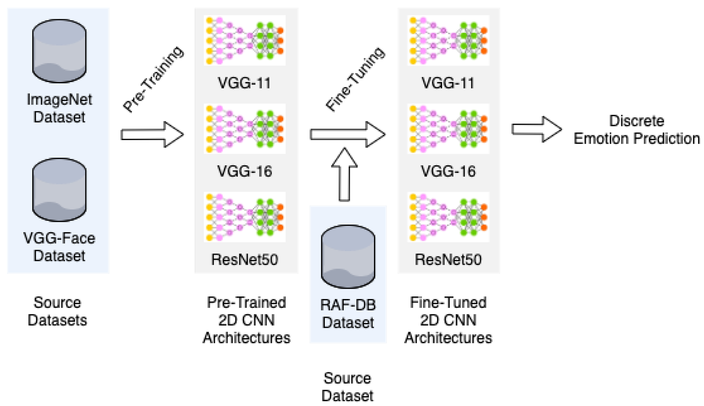
This paper proposes a two-step approach for continuous emotion prediction. In the first step, to circumvent the lack of sequences of continuous labeled videos, three source datasets, namely ImageNet, VGG-Face, and RAF-DB, are employed to initialize the 2D CNN architectures. ImageNet and VGG-Face datasets, which contain generic object images and face images, respectively, are used for pre-training three 2D CNN architectures: VGG-11, VGG-16, and ResNet50. These architectures were retained because they presented a state-of-the-art performance on discrete emotion recognition [42,46,47,61,62]. The RAF-DB dataset is closer to the target dataset since it contains face images annotated with discrete (categorical) emotions, and it is used for fine-tuning the 2D CNN architectures previously trained on ImageNet and VGG-Face datasets, as illustrated in Figure 2. Such 2D CNNs will be used as baseline models with the target dataset.
In the second step, such baseline models are extended to handle spatiotemporal information and perform continuous emotion recognition. Furthermore, such extended models are fine-tuned on a target dataset. There are two strategies to model the sequential information of videos, as shown in Figure 3: (i) a cascade approach, where an LSTM unit is added after the last convolutional layer of the 2D CNNs to form a 2D CNN–LSTM; (ii) inflating the 2D convolutional layers of the 2D CNNs to a third dimension to build an i3D CNN. This second step also includes the pre-processing of video frames, as well as post-processing predictions.
The rest of this section provides additional information on the pre-training and fine-tuning of 2D CNN models, the pre-processing steps to locate face images within video frames and build sequences of frames to feed spatiotemporal models, the DL models for continuous emotion recognition, and post-processing of the emotion predictions.

3.1. Pre-Training and Fine-Tuning of 2D CNNs

Training CNNs on small datasets systematically leads to overfitting. To circumvent this issue, CNNs can be pre-trained or fine-tuned on datasets that are similar or not to the target task [40,41]. Well-known CNN architectures, such as AlexNet [63], VGG [43], and GoogleNet, form an important set of baselines for a large number of tasks; in particular, pre-training such networks on the ImageNet dataset constitutes a powerful tool for representation learning. However, recent FER studies have shown that VGG-Face architectures, which are trained on a huge dataset of face images, overwhelms architectures trained on ImageNet for FER applications [64]. Furthermore, Li and Deng [1] showed that multi-stage fine-tuning can provide even better performance. Particularly, FER2013 [15], TFD [16] or, more recently, RAF-DB [65,66] datasets are good sources of additional data for FER tasks. Tannugi et al. [67] and Li and Deng [68] pursued interesting work on cross-dataset generalization tasks by switching in turn source and target FER datasets and evaluating the performance of FER models. Li and Deng [68] showed that datasets are strongly biased, and they developed a novel architecture that can learn domain-invariant and discriminative features.
Globally, this study considers using three different data sources for double transfer learning [69]: VGG-Face, ImageNet, and RAF-DB. There are already three architectures (VGG-11, VGG-16, and ResNet50) pre-trained on the first two datasets. However, such architectures had to be fully trained on the RAF-DB dataset. Several configurations were evaluated for training and fine-tuning different 2D CNN architectures on the RAF-DB dataset to determine how multi-stage fine-tuning can be well performed. The 2D CNN architectures were fine-tuned by freezing the weights of specific early layers while optimizing deeper ones. Since the three architectures have several convolutional blocks, the weights were frozen sequentially according to these blocks. The proposed architecture keeps convolutional blocks, while discriminant layers (i.e., fully connected layers) were replaced by a stack of two fully connected layers with 512 and 128 units, respectively, and an output layer with 7 units, since there are seven discrete emotion categories in the RAF-DB dataset: surprise, fear, disgust, happiness, sadness, anger, and neutral.

3.2. Pre-Processing

Face images are usually affected by background variations, such as illumination, head pose, and face patterns linked to identity bias. In this way, alignment and normalization are the two most commonly used preprocessing methods in face recognition, which may aid in learning discriminant features. For instance, the RAF-DB dataset contains aligned faces, while the subjects in the SEWA-DB dataset naturally face a web camera. Therefore, face alignment is not an important issue for this study. Furthermore, normalization only consists of scale pixel values between 0 and 1 to standardize input dimensions. Furthermore, faces were resized to 100 × 80 pixels, the average dimension of faces found in the target dataset. The details of other essential steps for facial expression recognition in video sequences, such as frame and face extraction and window bagging, are presented as follows.

3.2.1. Frame and Face Extraction

The videos of the target dataset (SEWA-DB) were recorded at 50 frames per second (fps). On the other hand, the valence and arousal annotations are available at an interval of 10 ms, corresponding to 10 fps. Therefore, it is necessary to replicate annotations for non-labeled frames when using 50 fps.
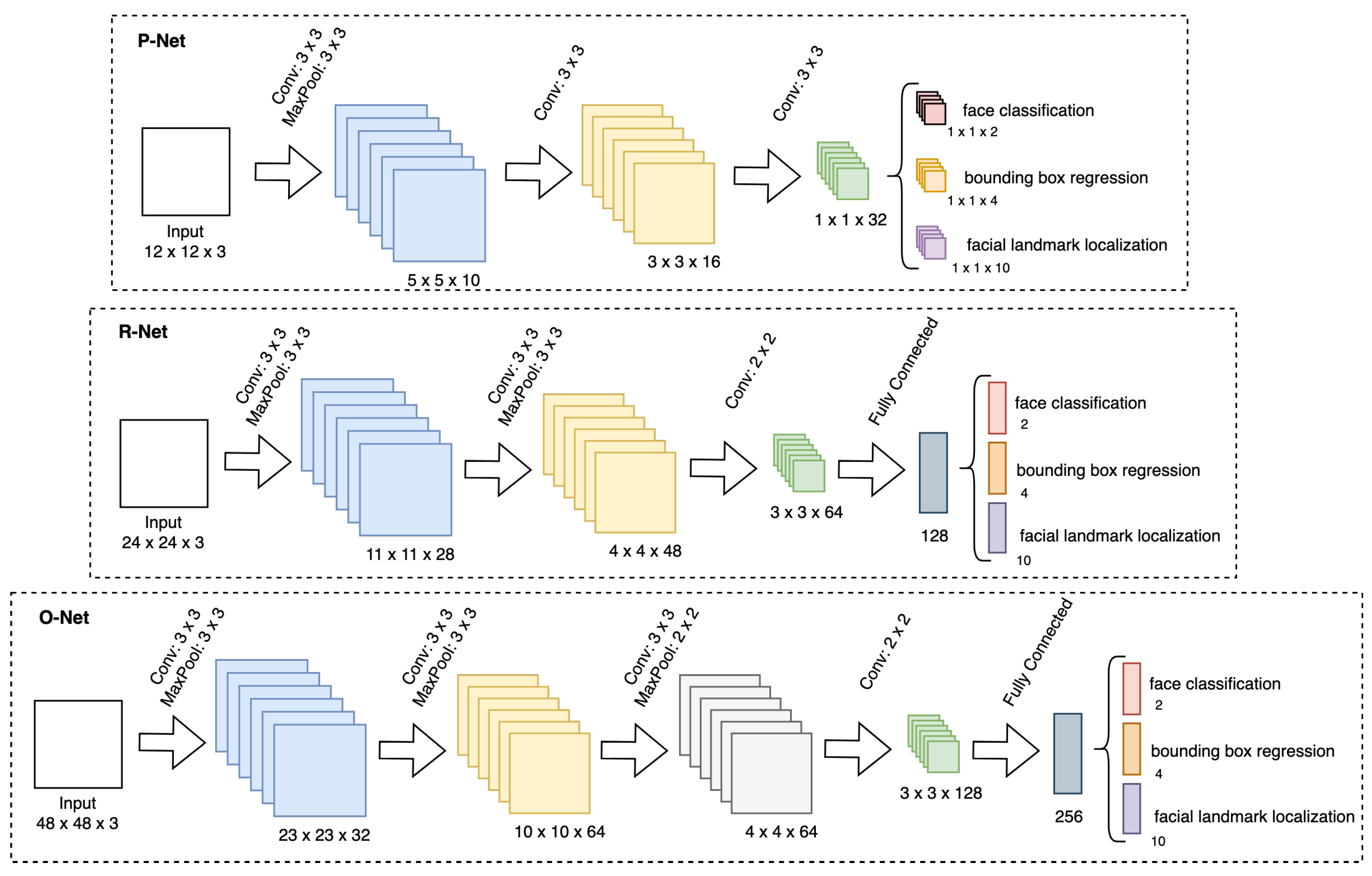
For locating and extracting faces from the frames of the SEWA-DB videos, it is employed a multi-task cascaded CNN (MTCNN) [70], which has shown excellent efficiency in electing the best bounding box candidates showing a whole face within the image. The MTCNN employs three CNNs sequentially to decide which bounding box must be kept according to particular criteria learned by deep learning. The face extractor network outputs box coordinates and five facial landmarks: eyes, nose, and mouth extremities. Once faces are located, they are cropped using the corresponding bounding box. An overview of MTCNN architecture is shown in Figure 4. Only frames showing whole faces are kept, while other frames are discarded.

3.2.2. Sequence Learning

The target dataset contains long video sequences showing a variety of emotions along with records of facial expressions from single subjects. The duration of emotions is not clearly established, and it varies for each individual. Several studies were previously carried out to obtain expression intensity variations by pointing peak and non-peak expressions along with sequences. However, while whole video sequences represent multiple annotations at a specific sampling rate and not a single label to describe a succession of diverse emotional states, the video sequences are split into several clips of fixed length with a specific overlapping ratio. This has two main advantages: (i) it increases the amount of data for training CNNs; (ii) it allows the investigation of which window settings are better for training spatiotemporal CNNs to learn from long sequences of valence and arousal annotations. Based on an exploratory study, two sequence lengths (16 and 64 consecutive frames of a single video) and three overlapping ratios for each sequence length (0.2, 0.5, and 0.8) were chosen. Thus, for instance, a window of 16 consecutive frames with an overlap of 0.5 contains the last eight frames of the previous window.
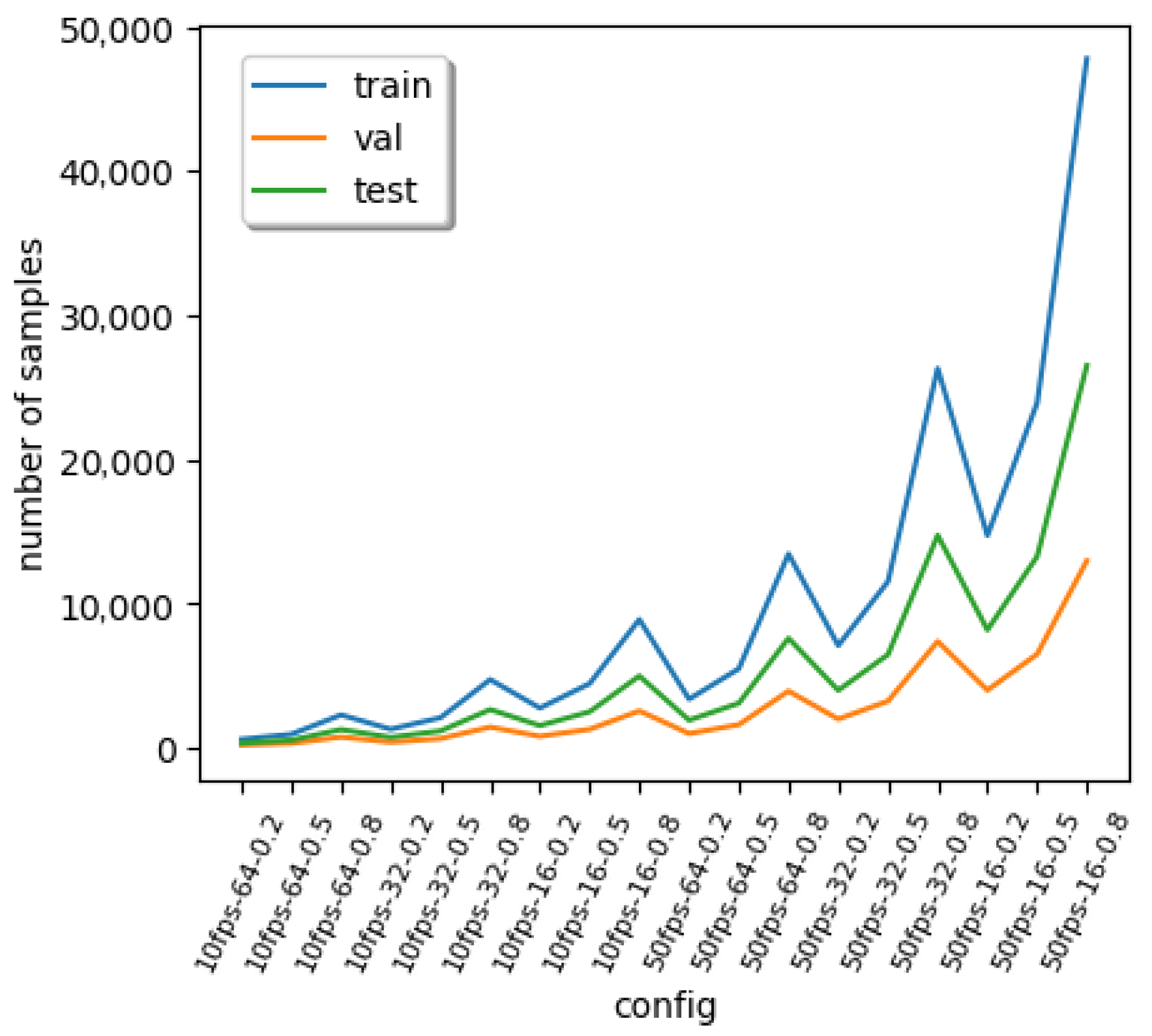
It is also important to check the integrity of contiguous video frames. Indeed, some frames were discarded because no face was detected within them, damaging the continuity of the temporal information of emotion between them. Furthermore, the proposed strategy to divide videos into clips may introduce critical temporal gaps between two consecutive frames. Therefore, a tolerance (a temporal difference between close frames) was applied to select clips that give sense to a unique emotion unit. Globally, the MTCNN can detect faces in videoclips, and on average, 90% of the frames are kept, depending on the sequence length, overlapping ratio, and frame rate. Figure 5 presents the number of clips available in training, validation, and test sets, according to such parameters. Finally, the last preprocessing step is to fuse annotations of multiple frames in one clip to obtain a single emotion label for each window. For such an aim, either the average or the extremum value of the labels is used to obtain a single label for each continuous emotion (single valence and arousal values).

3.3. Spatiotemporal Models

Two spatiotemporal models were developed: (i) a cascaded network based on a VGG-16 network pre-trained on VGG-Face that can be fine-tuned or not on the RAF-DB dataset; and (ii) an inflated network based on either VGG-11, VGG-16, or ResNet50 architectures pre-trained on different datasets (VGG-Face, RAF-DB, ImageNet).

3.3.1. Cascaded Networks (2D CNN–LSTM)

Long short-term memory units (LSTMs) are a special kind of RNN, capable of learning order dependence that may be found in a sequence of frames from a video. The core of LSTMs is a cell state, which adds or removes information depending on the input, output, and forget gates. The cell state remembers values over arbitrary time intervals, and the gates regulate the flow of input and output information of the cell.
The architecture of the proposed cascade network combines the 2D convolutional layers of VGG-16 for representation learning with an LSTM to support sequence prediction, as shown in Figure 6. Video frames are fed to the VGG-16-LSTM and then accumulated to form a feature vector representing one clip. After going through the LSTM unit for modeling temporal information between frames, the fully connected (FC) layers perform valence and arousal values regression. The LSTM has a single layer with 1024 units, with random and uniform distribution initialization to extract temporal features from the face features learned by the 2D CNN. In addition, some dropout (20%) and recurrent dropout (20%) were added on LSTM units to avoid overfitting. There are also three fully connected layers stacked after the LSTM to improve the expressiveness and accuracy of the model.
The VGG-16-LSTM architecture is pre-trained considering two different strategies: (i) VGG-16 pre-trained on the VGG-Face dataset; and (ii) VGG-16 pre-trained on the VGG-Face dataset and fine-tuned on the RAF-DB dataset. The former strategy adds extra information to the models, such as the classification of discrete emotions with RAF-DB, which could help to improve the performance on the regression task.

3.3.2. Inflated 3D CNN (i3D CNN)

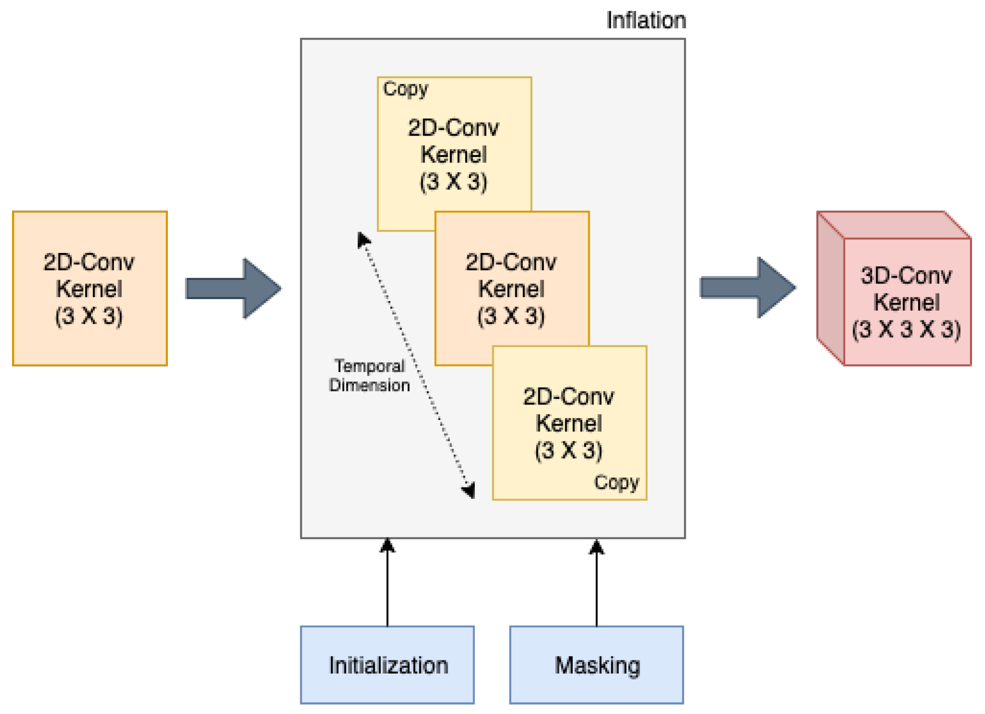
The need to analyze a sequence of frames led us to the use of 3D CNNs. Three-dimensional CNNs produce activation maps that allow analyzing data where temporal information is relevant. The main advantage of 3D CNNs is to learn representation from clips that can strengthen the spatiotemporal relationship between frames. Different from 2D CNNs, 3D CNNs are directly trained on batches of frame sequences rather than batches of frames. On the other hand, adding a third dimension to the CNN architecture increases the number of parameters of the model, and that requires much larger training datasets than those needed by 2D models. The main downside of using such an architecture for FER tasks is the lack of pre-trained models. Besides that, it is difficult to train 3D CNN architectures end to end for continuous emotion recognition, due to the limited amount of training data. Therefore, a feasible solution is to resort to weight inflation of 2D CNN pre-trained models [49]. Inflating a 2D CNN minimizes the need for large amounts of data for training a 3D CNN properly, as the inflation process reuses the weights of the 2D CNNs. Figure 7 shows that the weight inflation consists of enlarging kernels of each convolution filter by one dimension.
Our target task implies extending each neuron’s receptive field to the time dimension (i.e., a sequence of frames). The 2D convolutional kernels are replicated to fit the third dimension and form a 3D convolutional kernel. At first glance, pre-trained weights are just copied through the time dimension and provide a better approximation for initialization than randomness. However, they do not constitute an adequate distribution for the time dimension yet. With this in mind, the next issue is finding a method that best fits the transfer learning to the time dimension with weight inflation by varying some parameters, such as initialization, masking, multiplier, and dilation.
Initialization: When replicating kernels for weight inflation, it is possible to copy the weights n times (n being the dimension of the time axis) or to center the weights. Centering means copying once the weights of a 2D kernel and initializing the weights of the surrounding kernels that form the 3D filter either randomly (with a uniform distribution) or with zeros. Assuming that pre-trained 2D kernels have a good capacity for generalization for images, giving sufficiently distant distribution for all but one 2D kernel from the copied 2D kernel could positively impact model convergence.
Masking: Assuming that copied 2D kernels are pre-trained properly considering a very similar task and that they perform well on images, the idea of masking is to train adequately inflated weights on the time dimension. Therefore, to disseminate the spatial representation learned from pre-trained weights to inflated weights, centered weights are not modified during training.
Multiplier: The distribution of CNN weights and the range of targeted values for regression are closely related. Since values of valence and arousal range from 1 to 1 and standard values of the weights often take values between 10 3 and 10 1 , then rising targeted values by a factor could allow to scale up the distribution space and improve convergence.
Dilation: Dilated convolutions are used in our models, as suggested by Yu and Koltun [71]. The dilation was performed only on the time dimension.The architectures were divided into four blocks with increasing dilation levels, from 1 (no dilation) to 2, 4, and 8 for top convolutional layers. Dilated convolution consists of receptive fields larger than conventional ones. In other words, neuron connections of one convolutional layer are spread among neurons of previous layers. Notably, such a kind of implementation showed good performance for segmentation and object recognition tasks.
Figure 8 shows the architecture of the proposed i3D CNN, which is based on the inflation of 2D convolutional kernels of a pre-trained VGG-16 CNN. Video clips are fed to the i3D CNN, then spatiotemporal face features are extracted, and two fully connected (FC) layers perform the regression of valence and arousal values. Such an i3D CNN is then fine-tuned on a target dataset to perform the regression of valence and arousal values with a sequence of fully connected layers.

3.4. Post-Processing

The post-processing aims to improve the quality of the prediction by using some statistical information of the target dataset to reduce variance among datasets [72]. However, due to data imbalance in the training set, some valence and arousal values are difficult to reach. For instance, in the target dataset, neutral emotions, which imply valence and arousal levels close to zero, are much more frequent in the training set than extreme valence and arousal values (close to 1). Therefore, three post-processing steps are used to reduce the variance: scale normalization, mean filtering, and time delay.
Scale normalization consists in normalizing the predictions according to the distribution of the labels in the training set. Valence and arousal predictions ( y ) are normalized by the mean ( y ¯ l t r ) and the standard deviation ( σ l t r ) of the labels of the training set as:
y s n = y y ¯ l t r σ l t r
Mean filtering consists of centering predictions around mean values, increasing the linear relationship, and labeling correspondence. Valence and arousal predictions ( y ) are centered by subtracting the mean value of the labels ( y ¯ l t r ) of the training set and by adding the mean value of the predictions ( y ¯ t r ) on the training set as:
y m f = y y ¯ l t r + y ¯ t r
Finally, a time delay is used to compensate for some offset between labels and predictions due to the reaction lag of annotators. Valence and arousal predictions ( y ( f ) ) at frame f are shifted over t frames (precedent or subsequent) in order to align predictions and labels temporally as:
y t d = y ( f + t )
where t is an integer in [ 10 , 10 ] .

4. Experimental Results

This section briefly describes the two FER datasets used in the experiments: RAF-DB and SEWA-DB. Next, it presents the performance measures and summarizes our experimental setting and the results achieved by the proposed 2D CNN-LSTM and i3D CNN models

4.1. Facial Expression Datasets

The Real World Affective Faces Database (RAF-DB) is a real-world dataset that contains 29,672 images downloaded from the internet [65]. Around 40 annotators have labeled each image. The dataset has two types of annotation: 7 classes of basic emotions and 12 classes of compound emotions. Only the seven basic emotions (face images and labels) were used. Other metadata, such as facial landmarks, bounding box, and identity bias (e.g., age, gender, and race) are also provided, but they were not used in any step of the proposed approach. RAF-DB was used to fine-tune the pre-trained 2D CNNs.
SEWA-DB is a large and richly annotated dataset consisting of six groups of subjects (around 30 people per group) from six different cultural backgrounds (British, German, Hungarian, Greek, Serbian, and Chinese) divided into pairs of subjects [60]. Each pair of subjects discussed their emotional state and sentiment toward four previously watched adverts. The dataset consists of 64 videos (around 1525 minutes of audiovisual data) split into three folders (34 training, 14 validation, and 16 test). Since the labels are not provided for the test set due to its use in FER challenges, the validation set was used as the test set, and the training set was split into training (28 videos) and validation (6 videos) sets. In addition, annotations are given for valence, arousal, and levels of liking. Only valence and arousal annotations were used since previous studies indicated that the liking level is not well related to facial expressions.

4.2. Performance Metrics

The standard performance metrics used in continuous emotion recognition are the mean absolute error (MAE), the mean absolute percentage error (MAPE), Pearson correlation coefficient (PCC), and concordance correlation coefficient (CCC). PCC assesses the distance between target values and predictions, and CCC establishes the strength of a linear relationship between two variables. The range of possible values lies in the interval [ 1 ; 1 ] , where 1 or 1 means strong relation and 0 means no relation at all. The MAE for a set of labels y and predictions y is given by:
MAE = 1 n i = 1 n | y i y i |
The MAPE for a set of labels y and predictions y is given by:
MAPE = 1 n i = 1 n | y i y i | y i
The PCC is given as:
ρ = i = 1 n y i y ¯ y i y ¯ i = 1 n y i y ¯ 2 i = 1 n y i y ¯ 2
where n is the number of samples, y i is the i-th label, y i is the i-th prediction, and y ¯ and y ¯ are the mean of labels and mean of predictions, respectively. It is important to notice that these performance metrics are computed for each labeled video frame. Therefore, n represents the total number of video frames in a test dataset.
The CCC combines the PCC with the squared difference between the mean of predictions y ¯ and the mean of the labels y ¯ . CCC shows the degree of correspondence between the label and prediction distributions based on the covariance and correspondence. The CCC between a set of labels y and predictions y is given by:
ρ c = 2 ρ s y s y s y 2 + s y 2 + y ¯ y ¯ 2
where s y 2 and s y 2 are the variance of y and y respectively.

4.3. Training and Fine-Tuning 2D CNNs

Our first task is to specialize the three pre-trained CNN architectures (VGG-11, VGG-16, and ResNet50) for emotion recognition by fine-tuning them with the RAF-DB dataset. These three architectures were pre-trained either on the VGG-Face or ImageNet datasets. For fine-tuning the pre-trained 2D CNNs on the RAF-DB dataset, video frames were resized to 100 × 80 × 3, which is the mean dimension of video frames of the target dataset (SEWA-DB). The learning rate was fixed to 1 × 10 5 and batches of size 16. Optimization was performed with the Adam optimizer. Different weights were assigned to each class according to the number of samples to deal with the data imbalance found in the RAF-DB dataset. This allows classes with few samples to affect the model’s weights to the same extent as classes with many more samples. Moreover, low-level data augmentation, such as rotation, flipping, and highlight variations, can also help improve performance. Although data augmentation cannot bring important information for emotion recognition, it can prevent overfitting on a single sample and improve the model distributions.
Table 1 presents the performance achieved by the 2D CNNs after fine-tuning on the RAF-DB dataset, where the suffix BN refers to batch normalization layers added to the original architectures after each convolutional layer to improve model convergence and reduce overfitting. Furthermore, it is indicated for each architecture the dataset used for pre-training and the convolution block (2_1 to 5_1) where fine-tuning starts. In general, most fine-tuned models achieved an accuracy higher than the baseline models [62]. Jyoti et al. [62] developed two 2D CNNs to analyze action units’ detection efficiency on three datasets, including the RAF-DB dataset. The first CNN was based on residual connections with densely connected blocks (ResNet), and the second architecture was a 2D CNN consisting of four convolution layers and three fully connected layers. Such baselines achieved 76.54% and 78.23% accuracies on the RAF-DB test set, respectively. On the other hand, the proposed VGG-16 CNN model pre-trained with VGG-Face achieved 79.90% accuracy on the same test set.
Other recent works, which employed attention networks, achieved better performance [73,74]. However, the proposed approach did not consider two common problems in face analysis in real-world scenarios: occlusions and pose variations. On the contrary, Wang et al. [74] and Li et al. [73] addressed these problems using region-based attention networks. Attention modules are used to extract compact face representations based on several regions cropped from the face, and they adaptively adjust the importance of facial parts. Therefore, these models learn to discriminate occluded and non-occluded faces while improving emotion detection in both cases.

4.4. 2D CNN–LSTM Architecture

After specializing the three pre-trained CNN architectures (VGG-11, VGG-16, and ResNet50) for emotion recognition by fine-tuning them on the RAF-DB dataset, we developed cascaded networks based on such architectures for spatiotemporal continuous emotion recognition. Two 2D CNN–LSTM models were developed: (i) one based on the VGG-16 architecture pre-trained on the VGG-Face dataset and fine-tuned on the RAF-DB dataset because such an architecture achieved the best results on the RAF-DB test set; and (ii) a second one without fine-tuning on the RAF-DB dataset. The 2D CNN sequentially provides spatial features for each input frame, and the LSTM unit models the temporal information from a single clip. Different configurations were evaluated by varying the length of sequences, the overlapping ratio, and the strategy to fuse the labels within a clip. The architectures were fine-tuned on the development set of SEWA-DB, and the mean squared error (MSE) was used as a cost function. Some other works also considered CCC as a cost function [72] since it provides information about correspondence and correlation between predictions and annotations. However, a better convergence is observed while using the MSE.
Table 2 shows the results in terms of PCC and CCC, considering different frames rates (fps), sequence lengths (SL), overlapping ratios (OR), and fusion modes (FM). In general, both extremum and mean fusion performed well, and the best results for both valence and arousal were achieved for sequences of 64 frames at 10 fps. The VGG-16 architecture benefited from fine-tuning on the RAF-DB, and it achieved CCC values of 0.625 for valence and 0.557 for arousal on the validation set of SEWA-DB. In addition to the correlation metrics, the proposed 2D CNN–LSTM achieved an overall MAE of 0.06 (among 2D CNN–LSTM models), indicating a good correspondence between predictions and annotations. Since the best performance was obtained with post-processing steps, thus remodeling our set of predictions and annotations, MAPE was also computed to evaluate the error ratio between predictions and annotations.

4.5. i3D CNN Architecture

Another alternative for spatiotemporal modeling is to use the i3D CNN. In this way, strong spatiotemporal correlations between frames are directly learned from video clips by a single network. Thanks to weight inflation, the pre-trained 2D CNNs can be used to build i3D CNN architectures. The inflation method allows us to transpose learned information from various static tasks to dynamic ones, performing the essential transfer learning for learning spatiotemporal features. With this in mind, the 2D CNN architectures shown in Table 1 are reused, and their convolutional layers are expanded to build i3D CNNs considering two configurations, denoted as C1 and C2 in Table 3.
Due to the high number of trainable parameters, i3D CNNs are particularly time consuming to train. Therefore, some basic hyperparameters had a fixed value instead of performing exploratory experiments to set them. Consequently, we evaluated only the best configuration found for the 2D CNN–LSTM, as shown in Table 1, which uses a batch of size 8, a sequence length of 64 frames, overlapping ratio of 0.8, and frame rate of 10 fps. This is the main downside of our approach based on i3D CNNs. The number of trainable parameters of i3D CNNs is three times greater than the counterpart 2D CNNs.
Table 4 and Table 5 show only the best configurations of each architecture for valence and arousal prediction, respectively. These configuration were obtained from an exhaustive combination of the parameters’ values shown in Table 3 for each base model and considering different datasets for initializing such base models. Globally, different inflation types, masking, and dilation values do not impact the results achieved by i3D models. Table 6 shows the best performance obtained for each architecture for valence and arousal in terms of PCC and CCC values. Inflated 3D CNNs for regression seem sensitive to some training configurations regarding the range of results achieved by different base models and datasets used in their initialization. In these conditions, it is difficult to state the effect of a single parameter for inflation. VGG-16 with batch normalization and ResNet50 achieved the best results for valence and arousal and showed a good ability to predict these values, compared to other base models. Surprisingly, the VGG-16 pre-trained on ImageNet achieved higher PCC and CCC for both valence and arousal than those base models pre-trained on VGG-Face and RAF-DB, which are source datasets closer to the target one.
On the other hand, ResNet50 benefited from initialization with VGG-Face. In summary, the best results ranged from 0.313 to 0.406 for PCC and from 0.253 to 0.326 for CCC. The performance still shows a poor correlation between predictions and annotations. Still, it is comparable to the performance achieved by other studies on continuous emotion prediction that used the SEWA-DB dataset.

5. Discussion

The experiments carried out on SEWA-DB showed that the 2D CNN–LSTM architectures (Table 2) achieved better results than i3D CNN architectures (Table 6). Notably, for the former, valence was better predicted than arousal in terms of CCC. On the contrary, for the latter, arousal was better predicted than valence, also in terms of CCC. Previous works raised the fact that, intuitively, face textures on video sequences are the primary source of information for describing the level of positivity in emotions, hence the valence values. In contrast, arousal is better predicted with voice frequencies and audio signals. However, our work with inflated networks suggests that simultaneous learning of spatiotemporal face features benefits the prediction of arousal values.
Regarding the complexity of the two proposed approaches for continuous emotion recognition, we had to make some trade-off that certainly impacted the quality of the results provided by i3D CNN architectures. On the other hand, high sensitivity in training this type of architecture was also observed according to various configurations. This implies that i3D CNN architectures are very flexible, and further improvement could lie in better initialization and tuning of the number and quality of parameters regarding the potential of this model. Furthermore, inflated weights provided good initialization for action recognition tasks, suggesting that this method could also be utilized for emotion recognition. However, the main difference is that researchers had hundreds of short videos for a classification task for action recognition.
In contrast, we had relatively long videos of a few subjects for the regression task. Nevertheless, the experimental results showed great potential for further improvement if more data are available for fine-tuning the i3D models. On the other hand, the performance of 2D CNN–LSTM architectures was very satisfying, and this type of architecture is still a good choice for FER applications.
Table 7 shows the best results achieved by the proposed 2D CNN–LSTM and i3D CNN models and compares them with the baseline models proposed by Kossaifi et al. [60]. For ResNet18, they evaluated root mean squared error (RMSE) and CCC as loss functions. The CCCs achieved by the i3D CNN are slightly higher than those achieved by all models of Kossaifi et al. [60]. On the other hand, the CCC values achieved by the 2D CNN–LSTM are almost twice the best results achieved by the best model (ResNet18) of Kossaifi et al. [60]. Table 7 also shows the results achieved by [75,76], which are not directly comparable since both used a subset of SEWA-DB, encompassing only three cultures. They optimized emotion detection for two cultures (Hungarian and German) to perform well on the third one (Chinese). Notably, Ref. [75] proposed a combination of 2D CNN and 1D CNN, which has fewer parameters than 3D CNNs, and a spatiotemporal graph convolution network (ST-GCN) to extract appearance features from facial landmarks sequences. Ref. [76] used a VGG-style CNN and a DenseNet-style CNN to learn cross-culture face features, which were used to predict two adversarial targets: one for emotion prediction, another for culture classification. In conclusion, these two methodologies achieved state-of-the-art results on cross-cultural emotion prediction tasks.

6. Conclusions

This paper presented two CNN architectures for continuous emotion prediction in the wild. The first architecture is a combination of a fine-tuned VGG-16 CNN and an LSTM unit. This architecture achieved state-of-the-art results on the SEWA-DB dataset, producing CCC values of 0.625 and 0.557 for valence and arousal, respectively. The second architecture is based on the concept of inflation, which transfers knowledge from pre-trained 2D CNN models into a 3D one to model temporal features. The best proposed i3D CNN architecture achieved CCC values of 0.304 and 0.326 for valence and arousal prediction, respectively. These values are far below those achieved by the 2D CNN–LSTM. Due to the high number of parameters of i3D CNNs (barely three times greater than 2D CNNs), fine-tuning and hyperparameter tuning of such architectures require a substantial computational effort and massive datasets. Unfortunately, facial expression datasets for continuous emotion recognition are relatively small to accomplish such a task.
We also showed that a double transfer learning strategy over VGG and ResNet architectures with ImageNet and RAF-DB datasets can improve the accuracy of the baseline models. However, subjects mostly faced the camera with a relatively clear view of the whole face in this work. To some extent, this could imply some bias in the results when presenting diverse real-world scenarios. Moreover, the complexity of the i3D CNN architecture could, at this time, be a drag for live applications. Finally, to the best of our knowledge, it was the first time that 3D CNNs were used in regression applications for predicting valence and arousal values for emotion recognition.
There are some promising directions to expand the approaches proposed in this paper. For example, one could take advantage of the development of vast and complex cross-cultural datasets, such as the Aff-Wild dataset, to exploit occlusion cases, pose variations, or even scene breaks. We believe that i3D CNN architectures can deal with these specific cases, as they can learn discriminant spatiotemporal features that may improve separability. Furthermore, the recent Aff-Wild2 dataset, the largest existing in-the-wild video dataset, could also be used for pre-training the 2D CNNs on the same task (valence-arousal estimation) instead of using the RAF-DB dataset, which contains annotations for discrete emotion classification. Finally, the Aff-Wild2 dataset could also be used to train and evaluate the proposed 2D CNN–LTSM and i3D CNN architectures.
Finally, we showed a peculiar and flexible way of fine-tuning inflated CNNs; maybe this strategy could also be transferred to other applications, such as object and action recognition on video sequences.

Author Contributions

Conceptualization, T.T., É.G. and A.L.K.; methodology, T.T.; writing—original draft preparation, T.T.; writing—review and editing, A.L.K.; supervision, É.G. and A.L.K. All authors have read and agreed to the published version of the manuscript.

Funding

This research was partially funded by Natural Sciences and Engineering Research Council of Canada (NSERC) Discovery grant number RGPIN-2016-04855.

Institutional Review Board Statement

Not applicable.

Informed Consent Statement

Not applicable.

Data Availability Statement

All source code and CNN architectures described in this paper are available at https://github.com/alekoe/ster/ accessed on 8 December 2021. The SEWA database is available at https://db.sewaproject.eu accessed on 8 December 2021. The RAF database is available at http://www.whdeng.cn/raf/model1.html#dataset accessed on 8 December 2021. The VGG-Face dataset is available at https://www.robots.ox.ac.uk/~vgg/data/vgg_face/ accessed on 8 December 2021. The ImageNet database is available at https://image-net.org accessed on 8 December 2021.

Conflicts of Interest

The authors declare no conflict of interest.

References

  1. Li, S.; Deng, W. Deep facial expression recognition: A survey. arXiv 2018, arXiv:1804.08348. [Google Scholar] [CrossRef] [Green Version]
  2. Ekman, P.; Friesen, W.V. Constants across cultures in the face and emotion. J. Personal. Soc. Psychol. 1971, 17, 124–129. [Google Scholar] [CrossRef] [Green Version]
  3. Ekman, P. Strong evidence for universals in facial expressions: A reply to russell’s mistaken critique. Psychol. Bull. 1994, 115, 268–287. [Google Scholar] [CrossRef] [PubMed]
  4. Barrett, L.F.; Adolphs, R.; Marsella, S.; Martinez, A.M.; Pollak, S.D. Emotional Expressions Reconsidered: Challenges to Inferring Emotion From Human Facial Movements. Psychol. Sci. Public Interest 2019, 20, 1–68. [Google Scholar] [CrossRef] [Green Version]
  5. Barrett, L.F. AI weighs in on debate about universal facial expressions. Nature 2021, 589, 202–203. [Google Scholar] [CrossRef] [PubMed]
  6. Jack, R.E.; Garrod, O.G.; Yu, H.; Caldara, R.; Schyns, P.G. Facial expressions of emotion are not culturally universal. Proc Natl. Acad. Sci. USA 2012, 109, 7241–7244. [Google Scholar] [CrossRef] [PubMed] [Green Version]
  7. Warr, P.; Bindl, U.; Parker, S.; Inceoglu, I. Four-quadrant investigation of job-related affects and behaviours. Eur. J. Work Organ. Psychol. 2014, 23, 342–363. [Google Scholar] [CrossRef] [Green Version]
  8. Oliveira, L.E.S.; Mansano, M.; Koerich, A.L.; de Souza Britto, A. 2D Principal Component Analysis for Face and Facial-Expression Recognition. Comput. Sci. Eng. 2011, 13, 9–13. [Google Scholar] [CrossRef] [Green Version]
  9. Zavaschi, T.H.H.; Koerich, A.L.; Oliveira, L.E.S. Facial expression recognition using ensemble of classifiers. In Proceedings of the 2011 IEEE International Conference on Acoustics, Speech and Signal Processing (ICASSP), Prague, Czech Republic, 22–27 May 2011; pp. 1489–1492. [Google Scholar] [CrossRef] [Green Version]
  10. Shan, C.; Gong, S.; McOwan, P.W. Facial expression recognition based on local binary patterns: A comprehensive study. Image Vis. Comput. 2009, 27, 803–816. [Google Scholar] [CrossRef] [Green Version]
  11. Zavaschi, T.H.H.; Britto, A.S., Jr.; Oliveira, L.E.S.; Koerich, A.L. Fusion of feature sets and classifiers for facial expression recognition. Expert Syst. Appl. 2013, 40, 646–655. [Google Scholar] [CrossRef]
  12. Zhao, G.; Pietikainen, M. Dynamic Texture Recognition Using Local Binary Patterns with an Application to Facial Expressions. IEEE Trans. Pattern Anal. Mach. Intell. 2007, 29, 915–928. [Google Scholar] [CrossRef] [Green Version]
  13. Wang, Y.; See, J.; Phan, R.C.; Oh, Y. LBP with Six Intersection Points: Reducing Redundant Information in LBP-TOP for Micro-expression Recognition. In Proceedings of the 12th Asian Conference on Computer Vision, Singapore, 1–5 November 2014; Lecture Notes in Computer Science. Springer: Berlin/Heidelberg, Germany, 2014; Volume 9003, pp. 525–537. [Google Scholar] [CrossRef]
  14. Cossetin, M.J.; Nievola, J.C.; Koerich, A.L. Facial Expression Recognition Using a Pairwise Feature Selection and Classification Approach. In Proceedings of the IEEE International Joint Conference on Neural Networks (IJCNN), Vancouver, BC, Canada, 24–29 July 2016; pp. 5149–5155. [Google Scholar]
  15. Goodfellow, I.J.; Erhan, D.; Carrier, P.L.; Courville, A.C.; Mirza, M.; Hamner, B.; Cukierski, W.; Tang, Y.; Thaler, D.; Lee, D.; et al. Challenges in Representation Learning: A Report on Three Machine Learning Contests. In Proceedings of the 20th International Conference Neural Information Processing, Daegu, Korea, 3–7 November 2013; Lecture Notes in Computer Science. Springer: Berlin/Heidelberg, Germany, 2013; Volume 8228, pp. 117–124. [Google Scholar] [CrossRef] [Green Version]
  16. Susskind, J.M.; Anderson, A.K.; Hinton, G.E. The Toronto Face Dataset; Technical Report TR 2010-001; U. Toronto: Toronto, ON, Canada, 2010. [Google Scholar]
  17. Dhall, A.; Goecke, R.; Lucey, S.; Gedeon, T. Static facial expression analysis in tough conditions: Data, evaluation protocol and benchmark. In Proceedings of the IEEE International Conference on Computer Vision Workshops (ICCV Workshops), Barcelona, Spain, 6–13 November 2011; pp. 2106–2112. [Google Scholar]
  18. Georgescu, M.I.; Ionescu, R.T.; Popescu, M. Local Learning With Deep and Handcrafted Features for Facial Expression Recognition. IEEE Access 2019, 7, 64827–64836. [Google Scholar] [CrossRef]
  19. Kim, B.K.; Lee, H.; Roh, J.; Lee, S.Y. Hierarchical Committee of Deep CNNs with Exponentially-Weighted Decision Fusion for Static Facial Expression Recognition. In Proceedings of the International Conference on Multimodal Interaction, ICMI ’15, Seattle, WA, USA, 9–13 November 2015; pp. 427–434. [Google Scholar] [CrossRef]
  20. Liu, X.; Kumar, B.V.K.V.; You, J.; Jia, P. Adaptive Deep Metric Learning for Identity-Aware Facial Expression Recognition. In Proceedings of the IEEE Conference on Computer Vision and Pattern Recognition Workshops (CVPRW), Honolulu, HI, USA, 21–26 July 2017; pp. 522–531. [Google Scholar]
  21. Zhang, Z.; Luo, P.; Loy, C.C.; Tang, X. Learning Social Relation Traits from Face Images. In Proceedings of the IEEE International Conference on Computer Vision (ICCV), Santiago, Chile, 7–13 December 2015; pp. 3631–3639. [Google Scholar] [CrossRef] [Green Version]
  22. Guo, Y.; Tao, D.; Yu, J.; Xiong, H.; Li, Y. Deep Neural Networks with Relativity Learning for facial expression recognition. In Proceedings of the IEEE International Conference on Multimedia Expo Workshops (ICMEW), Seattle, WA, USA, 11–15 July 2016; pp. 1–6. [Google Scholar]
  23. Kim, B.; Dong, S.; Roh, J.; Kim, G.; Lee, S. Fusing Aligned and Non-aligned Face Information for Automatic Affect Recognition in the Wild: A Deep Learning Approach. In Proceedings of the IEEE Conference on Computer Vision and Pattern Recognition Workshops (CVPRW), Las Vegas, NV, USA, 26 June–1 July 2016; pp. 1499–1508. [Google Scholar]
  24. Pramerdorfer, C.; Kampel, M. Facial Expression Recognition using Convolutional Neural Networks: State of the Art. arXiv 2016, arXiv:1612.02903. [Google Scholar]
  25. Fayolle, S.L.; Droit-Volet, S. Time Perception and Dynamics of Facial Expressions of Emotions. PLoS ONE 2014, 9, e97944. [Google Scholar] [CrossRef] [Green Version]
  26. Bargal, S.A.; Barsoum, E.; Ferrer, C.C.; Zhang, C. Emotion Recognition in the Wild from Videos Using Images. In Proceedings of the International Conference on Multimodal Interaction, ICMI ’16, Tokyo, Japan, 12–16 November 2016; pp. 433–436. [Google Scholar] [CrossRef]
  27. Ding, W.; Xu, M.; Huang, D.Y.; Lin, W.; Dong, M.; Yu, X.; Li, H. Audio and Face Video Emotion Recognition in the Wild Using Deep Neural Networks and Small Datasets. In Proceedings of the 18th ACM International Conference on Multimodal Interaction, ICMI ’16, Tokyo, Japan, 12–16 November 2016; pp. 506–513. [Google Scholar] [CrossRef]
  28. Ayral, T.; Pedersoli, M.; Bacon, S.; Granger, E. Temporal Stochastic Softmax for 3D CNNs: An Application in Facial Expression Recognition. In Proceedings of the IEEE/CVF Winter Conference on Applications of Computer Vision, Waikola, HI, USA, 5–9 January 2021. [Google Scholar]
  29. Carneiro de Melo, W.; Granger, E.; Hadid, A. A Deep Multiscale Spatiotemporal Network for Assessing Depression from Facial Dynamics. IEEE Trans. Affect. Comput. 2020. [Google Scholar] [CrossRef]
  30. Tran, D.; Bourdev, L.D.; Fergus, R.; Torresani, L.; Paluri, M. Learning Spatiotemporal Features with 3D Convolutional Networks. In Proceedings of the IEEE International Conference on Computer Vision, (ICCV), Santiago, Chile, 7–13 December 2015; pp. 4489–4497. [Google Scholar] [CrossRef] [Green Version]
  31. Abbasnejad, I.; Sridharan, S.; Nguyen, D.; Denman, S.; Fookes, C.; Lucey, S. Using Synthetic Data to Improve Facial Expression Analysis with 3D Convolutional Networks. In Proceedings of the IEEE International Conference on Computer Vision Workshops (ICCVW), Venice, Italy, 22–29 October 2017; pp. 1609–1618. [Google Scholar]
  32. Fan, Y.; Lu, X.; Li, D.; Liu, Y. Video-Based Emotion Recognition Using CNN-RNN and C3D Hybrid Networks. In Proceedings of the International Conference on Multimodal Interaction, ICMI ’16, Tokyo, Japan, 12–16 November 2016; pp. 445–450. [Google Scholar] [CrossRef]
  33. Nguyen, D.; Nguyen, K.; Sridharan, S.; Ghasemi, A.; Dean, D.; Fookes, C. Deep Spatio-Temporal Features for Multimodal Emotion Recognition. In Proceedings of the 2017 IEEE Winter Conference on Applications of Computer Vision (WACV), Santa Rosa, CA, USA, 24–31 March 2017; pp. 1215–1223. [Google Scholar]
  34. Liu, K.; Liu, W.; Gan, C.; Tan, M.; Ma, H. T-C3D: Temporal Convolutional 3D Network for Real-Time Action Recognition. In Proceedings of the 32nd AAAI Conference on Artificial Intelligence, New Orleans, LA, USA, 2–7 February 2018; pp. 7138–7145. [Google Scholar]
  35. Barros, P.; Wermter, S. Developing crossmodal expression recognition based on a deep neural model. Adapt. Behav. 2016, 24, 373–396. [Google Scholar] [CrossRef] [PubMed]
  36. Zhao, J.; Mao, X.; Zhang, J. Learning deep facial expression features from image and optical flow sequences using 3D CNN. Vis. Comput. 2018, 34, 1461–1475. [Google Scholar] [CrossRef]
  37. Ouyang, X.; Kawaai, S.; Goh, E.; Shen, S.; Ding, W.; Ming, H.; Huang, D.Y. Audio-visual emotion recognition using deep transfer learning and multiple temporal models. In Proceedings of the 19th ACM International Conference on Multimodal Interaction, Glasgow, UK, 13–17 November 2017; pp. 577–582. [Google Scholar] [CrossRef]
  38. Ji, S.; Xu, W.; Yang, M.; Yu, K. 3D Convolutional Neural Networks for Human Action Recognition. IEEE Trans. Pattern Anal. Mach. Intell. 2013, 35, 221–231. [Google Scholar] [CrossRef] [Green Version]
  39. Vielzeuf, V.; Pateux, S.; Jurie, F. Temporal multimodal fusion for video emotion classification in the wild. In Proceedings of the 19th ACM International Conference on Multimodal Interaction (ICMI), Glasgow, UK, 13–17 November 2017; pp. 569–576. [Google Scholar] [CrossRef] [Green Version]
  40. Campos, V.; Salvador, A.; Giro-iNieto, X.; Jou, B. Diving deep into sentiment: Understanding fine-tuned CNNs for visual sentiment prediction. In Proceedings of the 1st International Workshop on Affect and Sentiment in Multimedia, Brisbane, Australia, 30 October 2015; pp. 57–62. [Google Scholar]
  41. Xu, C.; Cetintas, S.; Lee, K.C.; Li, L.J. Visual Sentiment Prediction with Deep Convolutional Neural Networks. arXiv 2014, arXiv:1411.5731. [Google Scholar]
  42. Parkhi, O.M.; Vedaldi, A.; Zisserman, A. Deep Face Recognition. In Proceedings of the British Machine Vision Conference (BMVC), Swansea, UK, 7–10 September 2015; pp. 41.1–41.12. [Google Scholar] [CrossRef] [Green Version]
  43. Simonyan, K.; Zisserman, A. Very Deep Convolutional Networks for Large-Scale Image Recognition. In Proceedings of the 3rd International Conference on Learning Representations, (ICLR), San Diego, CA, USA, 7–9 May 2015. [Google Scholar]
  44. Dhall, A.; Kaur, A.; Goecke, R.; Gedeon, T. EmotiW 2018: Audio-Video, Student Engagement and Group-Level Affect Prediction. In Proceedings of the International Conference on Multimodal Interaction (ICMI), Boulder, CO, USA, 16–20 October 2018; pp. 653–656. [Google Scholar] [CrossRef]
  45. Ringeval, F.; Schuller, B.; Valstar, M.; Jaiswal, S.; Marchi, E.; Lalanne, D.; Cowie, R.; Pantic, M. AV+EC 2015: The First Affect Recognition Challenge Bridging Across Audio, Video, and Physiological Data. In Proceedings of the 5th International Workshop on Audio/Visual Emotion Challenge, AVEC ’15, Brisbane, Australia, 26 October 2015; pp. 3–8. [Google Scholar] [CrossRef]
  46. Wan, L.; Liu, N.; Huo, H.; Fang, T. Face Recognition with Convolutional Neural Networks and subspace learning. In Proceedings of the 2nd International Conference on Image, Vision and Computing (ICIVC), Chengdu, China, 2–4 June 2017; pp. 228–233. [Google Scholar]
  47. Knyazev, B.; Shvetsov, R.; Efremova, N.; Kuharenko, A. Convolutional neural networks pretrained on large face recognition datasets for emotion classification from video. arXiv 2017, arXiv:1711.04598. [Google Scholar]
  48. Ding, H.; Zhou, S.K.; Chellappa, R. FaceNet2ExpNet: Regularizing a Deep Face Recognition Net for Expression Recognition. In Proceedings of the 12th IEEE International Conference on Automatic Face & Gesture Recognition, Washington, DC, USA, 30 May–3 June 2017; pp. 118–126. [Google Scholar] [CrossRef] [Green Version]
  49. Carreira, J.; Zisserman, A. Quo Vadis, Action Recognition? A New Model and the Kinetics Dataset. In Proceedings of the IEEE Conference on Computer Vision and Pattern Recognition, CVPR, Honolulu, HI, USA, 21–26 July 2017; pp. 4724–4733. [Google Scholar] [CrossRef] [Green Version]
  50. Diba, A.; Fayyaz, M.; Sharma, V.; Karami, A.H.; Arzani, M.M.; Yousefzadeh, R.; Gool, L.V. Temporal 3D ConvNets: New Architecture and Transfer Learning for Video Classification. arXiv 2017, arXiv:1711.08200. [Google Scholar]
  51. Praveen, G.; Granger, E.; Cardinal, P. Deep DA for Ordinal Regression of Pain Intensity Estimation Using Weakly-Labeled Videos. arXiv 2020, arXiv:2010.15675. [Google Scholar]
  52. Praveen, G.; Granger, E.; Cardinal, P. Deep Weakly-Supervised Domain Adaptation for Pain Localization in Videos. In Proceedings of the 15th IEEE International Conference on Automatic Face and Gesture Recognition (FG 2020), Buenos Aires, Argentina, 18–22 May 2020. [Google Scholar]
  53. Cardinal, P.; Dehak, N.; Koerich, A.L.; Alam, J.; Boucher, P. ETS System for AV+EC 2015 Challenge. In Proceedings of the ACM Multimedia Conference, Brisbane, Australia, 26–30 October 2015; pp. 17–23. [Google Scholar]
  54. Simonyan, K.; Zisserman, A. Two-Stream Convolutional Networks for Action Recognition in Videos. In Proceedings of the Advances in Neural Information Processing Systems 27: Annual Conference on Neural Information Processing Systems, Montreal, QC, Canada, 8–13 December 2014; pp. 568–576. [Google Scholar]
  55. Kim, H.; Kim, Y.; Kim, S.J.; Lee, I. Building Emotional Machines: Recognizing Image Emotions through Deep Neural Networks. IEEE Trans. Multim. 2018, 20, 2980–2992. [Google Scholar] [CrossRef] [Green Version]
  56. Mou, W.; Celiktutan, O.; Gunes, H. Group-level arousal and valence recognition in static images: Face, body and context. In Proceedings of the 2015 11th IEEE International Conference and Workshops on Automatic Face and Gesture Recognition (FG), Ljubljana, Slovenia, 4–8 May 2015; Volume 5, pp. 1–6. [Google Scholar]
  57. Ben Henia, W.M.; Lachiri, Z. Emotion classification in arousal-valence dimension using discrete affective keywords tagging. In Proceedings of the International Conference on Engineering MIS (ICEMIS), Monastir, Tunisia, 8–10 May 2017; pp. 1–6. [Google Scholar]
  58. Kollias, D.; Zafeiriou, S. A Multi-component CNN-RNN Approach for Dimensional Emotion Recognition in-the-wild. arXiv 2018, arXiv:1805.01452. [Google Scholar]
  59. Kollias, D.; Tzirakis, P.; Nicolaou, M.A.; Papaioannou, A.; Zhao, G.; Schuller, B.; Kotsia, I.; Zafeiriou, S. Deep Affect Prediction in-the-Wild: Aff-Wild Database and Challenge, Deep Architectures, and Beyond. Int. J. Comput. Vis. 2019, 127, 907–929. [Google Scholar] [CrossRef] [Green Version]
  60. Kossaifi, J.; Schuller, B.W.; Star, K.; Hajiyev, E.; Pantic, M.; Walecki, R.; Panagakis, Y.; Shen, J.; Schmitt, M.; Ringeval, F.; et al. SEWA DB: A Rich Database for Audio-Visual Emotion and Sentiment Research in the Wild. IEEE Trans. Pattern Anal. Mach. Intell. 2019. [Google Scholar] [CrossRef] [Green Version]
  61. Cao, Q.; Shen, L.; Xie, W.; Parkhi, O.M.; Zisserman, A. VGGFace2: A Dataset for Recognising Faces across Pose and Age. In Proceedings of the 13th IEEE International Conference on Automatic Face & Gesture Recognition, Xi’an, China, 15–19 May 2018; pp. 67–74. [Google Scholar] [CrossRef] [Green Version]
  62. Jyoti, S.; Sharma, G.; Dhall, A. Expression Empowered ResiDen Network for Facial Action Unit Detection. In Proceedings of the 14th IEEE International Conference on Automatic Face & Gesture Recognition, Lille, France, 14–18 May 2019; pp. 1–8. [Google Scholar] [CrossRef] [Green Version]
  63. Krizhevsky, A.; Sutskever, I.; Hinton, G.E. ImageNet Classification with Deep Convolutional Neural Networks. Commun. ACM 2017, 60, 84–90. [Google Scholar] [CrossRef]
  64. Kaya, H.; Gürpınar, F.; Salah, A. Video-Based Emotion Recognition in the Wild using Deep Transfer Learning and Score Fusion. Image Vis. Comput. 2017, 65, 66–75. [Google Scholar] [CrossRef]
  65. Li, S.; Deng, W.; Du, J. Reliable Crowdsourcing and Deep Locality-Preserving Learning for Expression Recognition in the Wild. In Proceedings of the IEEE Conference on Computer Vision and Pattern Recognition (CVPR), Honolulu, HI, USA, 21–26 July 2017; pp. 2584–2593. [Google Scholar]
  66. Li, S.; Deng, W. Reliable Crowdsourcing and Deep Locality-Preserving Learning for Unconstrained Facial Expression Recognition. IEEE Trans. Image Process. 2019, 28, 356–370. [Google Scholar] [CrossRef]
  67. Tannugi, D.L.; Britto, A.S., Jr.; Koerich, A.L. Memory Integrity of CNNs for Cross-Dataset Facial Expression Recognition. In Proceedings of the IEEE International Conference on Systems, Man, and Cybernetics (SMC), Bari, Italy, 6–9 October 2019; pp. 3806–3811. [Google Scholar]
  68. Li, S.; Deng, W. A Deeper Look at Facial Expression Dataset Bias. IEEE Trans. Affect. Comput. 2020. [Google Scholar] [CrossRef] [Green Version]
  69. de Matos, J.; Britto, A.S., Jr.; Oliveira, L.E.S.; Koerich, A.L. Double Transfer Learning for Breast Cancer Histopathologic Image Classification. In Proceedings of the IEEE International Joint Conference on Neural Networks (IJCNN), Budapest, Hungary, 14–19 July 2019; pp. 1–6. [Google Scholar]
  70. Zhang, K.; Zhang, Z.; Li, Z.; Qiao, Y. Joint face detection and alignment using multitask cascaded convolutional networks. IEEE Signal Process. Lett. 2016, 23, 1499–1503. [Google Scholar] [CrossRef] [Green Version]
  71. Yu, F.; Koltun, V. Multi-Scale Context Aggregation by Dilated Convolutions. In Proceedings of the 4th International Conference on Learning Representations (ICLR), San Juan, Puerto Rico, 2–4 May 2016. [Google Scholar]
  72. Ortega, J.D.S.; Cardinal, P.; Koerich, A.L. Emotion Recognition Using Fusion of Audio and Video Features. In Proceedings of the IEEE International Conference on Systems, Man, and Cybernetics (SMC), Bari, Italy, 6–9 October 2019; pp. 3827–3832. [Google Scholar]
  73. Li, Y.; Zeng, J.; Shan, S.; Chen, X. Occlusion Aware Facial Expression Recognition Using CNN With Attention Mechanism. IEEE Trans. Image Process. 2019, 28, 2439–2450. [Google Scholar] [CrossRef] [PubMed]
  74. Wang, K.; Peng, X.; Yang, J.; Meng, D.; Qiao, Y. Region Attention Networks for Pose and Occlusion Robust Facial Expression Recognition. IEEE Trans. Image Process. 2020, 29, 4057–4069. [Google Scholar] [CrossRef] [PubMed] [Green Version]
  75. Chen, H.; Deng, Y.; Cheng, S.; Wang, Y.; Jiang, D.; Sahli, H. Efficient Spatial Temporal Convolutional Features for Audiovisual Continuous Affect Recognition. In Proceedings of the 9th International on Audio/Visual Emotion Challenge and Workshop, AVEC ’19, Nice, France, 21 October 2019; pp. 19–26. [Google Scholar] [CrossRef] [Green Version]
  76. Zhao, J.; Li, R.; Liang, J.; Chen, S.; Jin, Q. Adversarial Domain Adaption for Multi-Cultural Dimensional Emotion Recognition in Dyadic Interactions. In Proceedings of the 9th International on Audio/Visual Emotion Challenge and Workshop, AVEC ’19, Nice, France, 21 October 2019; pp. 37–45. [Google Scholar] [CrossRef] [Green Version]
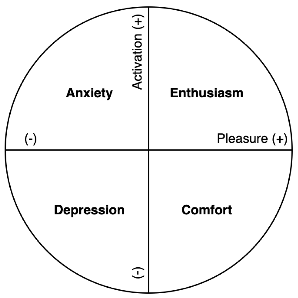
Figure 1. The circumplex model. Adapted from [7].
Applsci 11 11738 g001
Figure 2. Overview of pre-training and fine-tuning of 2D CNN architectures for discrete emotion prediction.
Applsci 11 11738 g002
Figure 3. Overview of the two used deep architectures for depicting spatiotemporal features on video sequences: a cascaded network 2D CNN–LSTM and an i3D CNN.
Applsci 11 11738 g003
Figure 4. Exhaustive MTCNN architecture composed of a stack of CNNs. A single meaningful bounding box and five facial landmarks are extracted from face images. Adapted from [70].
Applsci 11 11738 g004
Figure 5. Evolution of the number of sequences for training, validation and test sets for different configurations: 10 and 50 fps; sequence length of 16, 32 and 64 frames; overlapping ratio of 20%, 50% and 80%.
Applsci 11 11738 g005
Figure 6. The architecture of the VGG-16-LSTM. A 3 × 3 kernel is used in each convolutional layer. The numbers of filters and units in LSTM and FC layers are also indicated.
Applsci 11 11738 g006
Figure 7. Representation of the inflation method for a single convolutional filter. The 2D convolutional kernels are replicated along a new dimension (temporal dimension) to obtain 3D convolutional kernels. Basically, n × n kernels are made cubic to obtain n × n × n kernels. This process is applied to every convolutional filter to transform 2D convolutional layers into 3D convolutional layers.
Applsci 11 11738 g007
Figure 8. The proposed i3D CNN based on the inflation of the 2D convolutional kernels of a pre-trained VGG-16 CNN. For each convolutional layer, a 3 × 3 × 3 kernel is used. The numbers of filters and units in FC layers are also indicated.
Applsci 11 11738 g008
Table 1. Results of the fine-tuning of VGG and ResNet50 models on RAF-DB. Convolution block denotes the initial level of fine-tuning of each model. Full denotes that all layers were fine-tuned.
Reference ModelDataset for
Pre-Training
Convolution
Block
Accuracy (%)
ProposedVGG-11ImageNetFull
Conv_2_1
Conv_3_1
Conv_4_1
Conv_5_1
75.6
75.9
75.9
75.9
70.3
VGG-11-BNImageNetFull77.8
VGG-16VGG-FaceFull
Conv_2_1
Conv_3_1
Conv_4_1
Conv_5_1
78.5
78.5
79.1
79.9
74.4
VGG-16-BNVGG-FaceFull78.4
ResNet50VGG-FaceFull
Conv_4_1
Conv_5_1
79.7
78.0
65.1
Jyoti et al. [62]RCNNNANA76.5
CNNNANA78.2
Li et al. [73]ACNNImageNetNA85.1
Wang et al. [74]CNN+RANMS-Celeb-1MNA86.9
The level of schooling refers to the mothers of all schoolchildren, who are used as a proxy for socio-economic status.
Table 2. Performance of the 2D CNN–LSTM based on the VGG-16 architecture on the SEWA-DB dataset. The best results for valence and arousal are in boldface.
Dataset for
Initialization
Configuration
fpsLabel(SL, OR, FM)PCC↑CCC↑MAPE(%)↓
VGG-Face10Valence16, 0.2, extremum0.5900.5603.8
Arousal16, 0.2, mean0.5490.5428.7
50Valence64, 0.2, mean0.5410.5116.8
Arousal64, 0.2, extremum0.4950.4923.4
RAF-DB10Valence64, 0.8, mean0.6310.6253.7
Arousal64, 0.8, extremum0.5580.5579.4
50Valence64, 0.2, mean0.5820.5688.2
Arousal64, 0.2, extremum0.5170.5174.4
SL: sequence length (in frames), OR: overlapping ratio, FM: fusion mode.
Table 3. Hyperparameters of i3D CNN architectures and their possible values.
ParametersC1C2
InflationCenteredCopied
Weight InitializationRandomZero
MaskingNoYes
DilationBloc1: 1
Bloc2: 1
Bloc3: 1
Bloc4: 1
Bloc1: 1
Bloc2: 2
Bloc3: 4
Bloc4: 8
Multiplier×1×100
Table 4. The i3D CNN model configurations according to the best performance for predicting valence.
Parameters
Base ModelsDataset for InitializationModels InflationDilation MaskingInitialization Centered WeightsMult
VGG-11-BNRAF-DBCenteredINoZero×1
ImageNetCopiedINoZero×100
VGG-16VGG-FaceCenteredINoRandom×1
RAF-DBCopiedINoRandom×1
ImageNetCenteredINoRandom×1
VGG-16-BNVGG-FaceCenteredINoRandom×1
RAF-DBCopiedIYesRandom×1
ImageNetCopiedINoRandom×1
ResNet50VGG-FaceCenteredIYesZero×100
RAF-DBCopiedVIIINoZero×1
ImageNetCenteredVIIIYesZero×1
Table 5. The i3D CNN model configurations according to the best performance for predicting arousal.
Parameters
Base ModelsDataset for Initialization Inflation Dilation MaskingInitialization Centered Weights Mult
VGG-11-BNRAF-DBCenteredINoRandom×1
ImageNetCenteredVIIINoZero×1
VGG-16VGG-FaceCenteredINoRandom×1
RAF-DBCopiedIYesRandom×100
ImageNetCenteredINoRandom×1
VGG-16-BNVGG-FaceCenteredIYesRandom×1
RAF-DBCopiedINoRandom×1
ImageNetCenteredINoZero×1
ResNet50VGG-FaceCopiedIYesZero×100
RAF-DBCenteredVIIIYesZero×1
ImageNetCenteredINoZero×1
Table 6. Best performance of i3D CNNs for predicting valence and arousal in terms of PCC and CCC values and MAPE according to different models and their initialization. The higher values of PCC and CCC are in boldface.
ValenceArousal
Base ModelsDataset for InitializationPCC↑CCC↑MAPE(%)↓PCC↑CCC↑MAPE(%)↓
VGG-11-BNRAF-DB0.0350.0182.90.3590.3488.1
ImageNet0.0400.0254.20.3420.2033.0
VGG-16VGG-Face0.1190.0713.00.2200.1665.2
RAF-DB0.0360.0283.50.2420.1194.6
ImageNet0.2090.1902.40.3910.1893.8
VGG-16-BNVGG-Face0.2030.1053.60.3470.3045.3
RAF-DB0.1230.1013.20.2840.1653.3
ImageNet0.3460.3045.60.3820.3265.3
ResNet50VGG-Face0.3130.2533.50.4060.2734.9
RAF-DB0.1130.0632.90.2620.2074.9
ImageNet0.1830.1646.00.3230.2564.7
Table 7. Comparison of the best results achieved by the proposed models and the state-of-the-art for the SEWA-DB dataset. The best results for valence and arousal are in boldface.
ValenceArousal
ReferenceModelPCC↑CCC↑PCC↑CCC↑
Proposed2D-CNN-LSTM 1 0.6310.6250.5580.557
i3D-CNN 2 0.3460.3040.3820.326
Kossaifi et al. [60]SVR0.3210.3120.1820.202
RF0.2680.2070.1810.123
LSTM0.3220.2810.1730.115
ResNet18 (RMSE)0.2900.2700.1300.110
ResNet18 (CCC)0.3500.3500.3500.290
Chen et al. [75] ST-GCNNA0.540NA0.581
Zhao et al. [76] DenseNet-style CNNNA0.580NA0.594
1 VGG-16 fine-tuned with RAF-DB. 2 Inflated VGG-16-BN, initialized with ImageNet. NA: Not Available. Results are reported for a subset of SEWA-DB encompassing only three cultures (Hungarian, German, Chinese).
Publisher’s Note: MDPI stays neutral with regard to jurisdictional claims in published maps and institutional affiliations.