Numerical Integration-Based Performance Analysis of Cross-Eye Jamming Algorithm

Abstract

In this paper, performance analysis of the cross-eye jamming effect under mechanical defects is dealt with. By using a numerical analysis-based approach, the performance analysis method proposed in this paper is closer to the not approximated empirical mean square difference (MSD) than the first-order Taylor approximation-based performance analysis method and the second-order Taylor approximation-based performance analysis method proposed in previous studies. In other words, the effects of amplitude ratio perturbation and phase difference perturbation on performance degradation are quantitatively analyzed. Note that the numerical integration is adopted to derive an analytic expression of the MSD.

1. Introduction

The radar receives information on the target’s direction, distance, and velocity by using electromagnetic waves. The radar uses the received information to search and track the targets. Amplitude-comparison monopulse (ACM) radar is one of the tracking radars. The ACM uses only one pulse to measure the tracking error of a target accurately. ACM’s antenna consists of four beam patterns, which have the same squint angle. ACM can estimate the angle of the target by comparing the sum and difference of the received signals from each antenna for each pulse of the reflected signal [1].

In [2], multiple antennas in the ACM are used to estimate the angle of the target. In this way, the radar estimates the distance, velocity, and angle of the target and provides information to the guided weapon. This information poses a great threat to our ships and planes, so it is essential to disrupt the radar. In order to avoid ACM tracking, the target needs to disturb the ACM. A way to protect our ships from ACM is jamming, among which angle disturbances are effective. However, ACM calculates the sum pattern and the difference pattern from a single receiving pulse to estimate the angle, so the effect of the amplitude change between pulses is small. Cross eye jamming can effectively interfere with ACM’s angular tracking by changing the value of the received sum and difference of the ACM sensor [3,4,5,6,7].

Cross-eye is a method that causes the ACM to track the wrong angle. Cross-eye jamming causes angle errors, allowing the ACM to measure the false position of a target rather than the true position of the target through induced angle errors. The cross-eye jamming radiates jamming signals using two separate transmitters to ACM. At this time, because the phase difference between the two transmitters is 180°, propagation is distorted when the ACM receives a signal. The jamming signal generated by the cross-eye’s jammer antenna changes the sum of reception of the ACM and the value of the difference, causing an angle error [3,4,5,6,7,8,9,10].

The jammer antenna in the cross-eye that generates the deceiving signal is located on board ship at a distance of L. The disturbed angle caused by the signal from the jamming antenna will deceive the actual target’s position. The cross-eye gain is obtained by using the two jammer antenna’s jamming signals which have the amplitude ratio, a, and phase difference, $\varphi$. Because the cross-eye gain is the function of two variables, cross-eye jamming performance is greatly influenced by a and $\varphi$. It is the most effective when variable a is a unity and variable $\varphi$ is $\pi$ [11,12]. Variables a and $\varphi$ may differ from the nominal values of $a_0$ and ${\varphi }_0$ due to various reasons. The difference between a and $a_0$ can be modeled as a zero-mean Gaussian random variable. Similarly, the difference between $\varphi$ and ${\varphi }_0$ can be modeled as a zero-mean Gaussian random variable. The amount of degradation is dependent on the deviation of actual values of a and $\varphi$ from nominal values of a and $\varphi$. Many studies on the performance analysis of cross-eye gain have been conducted [11,12,13]. Previous studies focused on how to maximize cross-eye gain to prevent monopulse radars from accurately tracking angles by increasing the cross-eye gain. In contrast, this paper does not focus on increasing the value of cross-eye gain by controlling a and $\varphi$. In this paper, we are concerned with how the perturbations in a value and $\varphi$ value degrade the performance of the cross-eye jammer. More specifically, we are concerned the quantitative description of the performance degradation due to the difference between the nominal values and the true values of a and $\varphi$.

To get an analytic expression of the mean square difference (MSD), the Taylor approximation should be applied to the cross-eye gain expression. Because the cross-eye gain is a non-linear function expressed in fractional form, it is difficult to obtain closed-form analytic expression of the MSD. Therefore, after approximating the cross-eye gain as a polynomial function for a and $\varphi$ using the first-order and the second-order Taylor approximation, the analytical expansion of the expectation operator can be achieved. The Monte-Carlo simulation method is used to obtain the simulation MSD without approximation, the first-order Taylor approximation, and the second-order Taylor approximation cross-eye gain. The analytic expressions of MSD are given as explicit expressions in terms of the variance of the amplitude ratio, a, and phase difference, $\varphi$. Numerical integration-based MSD of cross-eye gain was obtained from numerical integration. Using joint PDF of two random variables of a and $\varphi$, the mean of functions consisting of two random variables, a and $\varphi$, is calculated. In order to analyze the accuracy of the cross-eye jamming effect under various mechanical defects the performance degradation of the cross-eye jamming was evaluated for several values of standard deviations. In the previous study [14], the analytic expression of MSD is obtained via the first order and the second order Taylor series, and the validity of the derived expression is shown by comparing the analytic results and the Monte-Carlo simulation-based results. In order to improve the accuracy of the MSD calculation, we propose a numerical integration-based MSD of cross-eye gain. In the previous study [14], the authors derived a close form expression of the analytic MSDs associated with the simulation based on the first-order Taylor expansion and with the simulation based on the second-order Taylor expansion. Note that the simulation based on the first-order Taylor expansion and the second-order Taylor expansion is slightly different from the simulation with non-approximation.

In [14], the authors proposed how the closed-form expression of the analytic MSD associated with the simulation based on the first-order Taylor expansion and the second-order Taylor expansion can be derived. In this paper, it is shown how the closed-form expression of the analytic MSD associated with the simulation with non-approximation can be expressed.

The computation time of MSD using an analytical method is much less than that of MSD calculated by the Monte-Carlo method with a large number of repetitions. In other words, the scheme in [14] has demonstrated that analytical MSDs have significantly less computational complexity than the Monte-Carlo simulation-based MSD. However, accuracy is reduced because of approximation. There is a difference between the non-approximated simulation-based MSD and the analytic-based approximated MSD. From that point of view, the accuracy is reduced. Therefore, we improve the MSD calculation accuracy of the cross-eye gain by considering the perturbation through numerical integration-based method. It does not mean that the integral method’s estimated performance is better than the analytic method’s one. The important point is that it is closer to the non-approximated simulation-based MSD than the analytic method. In this paper, how close various MSDs are to the MSD with non-approximation is the concern.

In Section 2, the cross-eye jamming method is briefly introduced, and why the cross-eye gain affects the cross-eye jamming performance. Further, MSD of approximated cross-eye gain, and non-approximated cross-eye gain are derived, respectively. In Section 3, numerical integration-based MSD, which uses joint PDF of two Gaussian random variables is derived. In Section 4, the result of each MSD is shown, and the performance of analytic MSDs, numerical integration-based MSD and simulation MSD are analyzed. Finally, in the conclusion, we summarize the overall contents of this paper and emphasize the advantages of the numerical integration-based MSD method compared to Monte-Carlo simulation-based MSD and analytic-based approximated MSD.

2. Cross-Eye Gain

In this section, cross-eye gain is defined, and MSD is defined as Equations (1)–(5). Cross-eye jamming can deceive the monopulse’s angle tracking. Cross-eye jamming is implemented by placing two jamming antennas on board ship. The jamming antennas radiate the jamming signal.

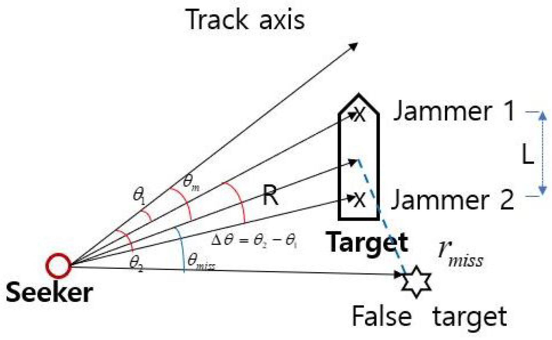
Figure 1 is a brief description of the cross-eye jamming technique. A false target is created by two jammer antennas on the board ship separated by distance L. Figure 1 shows that L is similar to the length of the ship, and is drawn to explain that cross-eye jammer antennas are on the board ship. Miss distance and miss angle are given by [1].

$$r_{\mathrm{miss}}=\frac{Lcos\psi }{2}\frac{1-a^2}{1+2acos\varphi +a^2}$$

(1)

$${\theta }_{\mathrm{miss}}=\frac{\Delta \theta }{2}\frac{1-a^2}{1+2acos\varphi +a^2}$$

(2)

where $\psi$ is the angle between the track axis and the line that is vertically bisected between the two jammers and $\Delta \theta$ is the angle between the two jammers. $r_{\mathrm{miss}}$ and ${\theta }_{\mathrm{miss}}$ have a common term, $\frac{1-a^2}{1+2acos\varphi +a^2}$, which is the cross-eye gain term

$$GC(a,\varphi )=\frac{1-a^2}{1+2acos\varphi +a^2}.$$

(3)

Thus, $r_{\mathrm{miss}}$ and ${\theta }_{\mathrm{miss}}$ can be simplified as

$$\begin{array}{c}\hfill r_{\mathrm{miss}}=\frac{Lcos\psi }{2}GC\end{array}$$

(4)

$$\begin{array}{c}\hfill {\theta }_{\mathrm{miss}}=\frac{\Delta \theta }{2}GC.\end{array}$$

(5)

Since $r_{\mathrm{miss}}$ and ${\theta }_{\mathrm{miss}}$ are functions of a and $\varphi$, it is greatly affected by the a and $\varphi$.

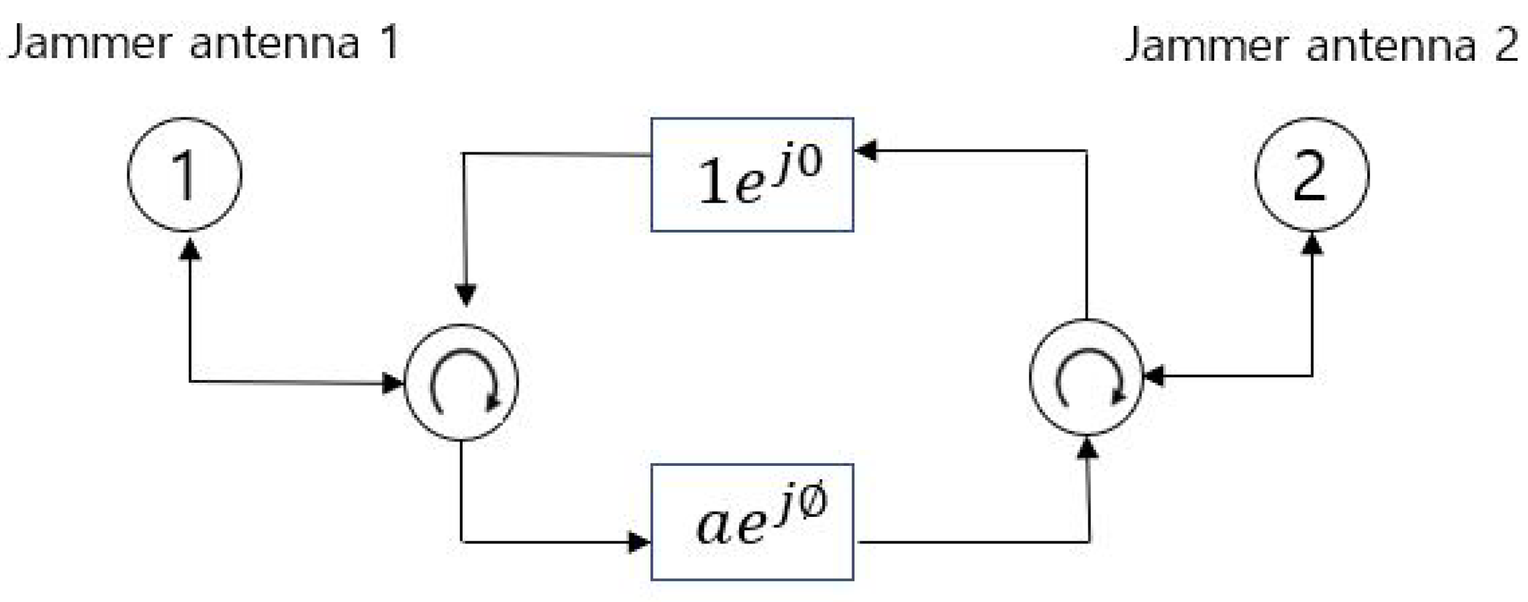
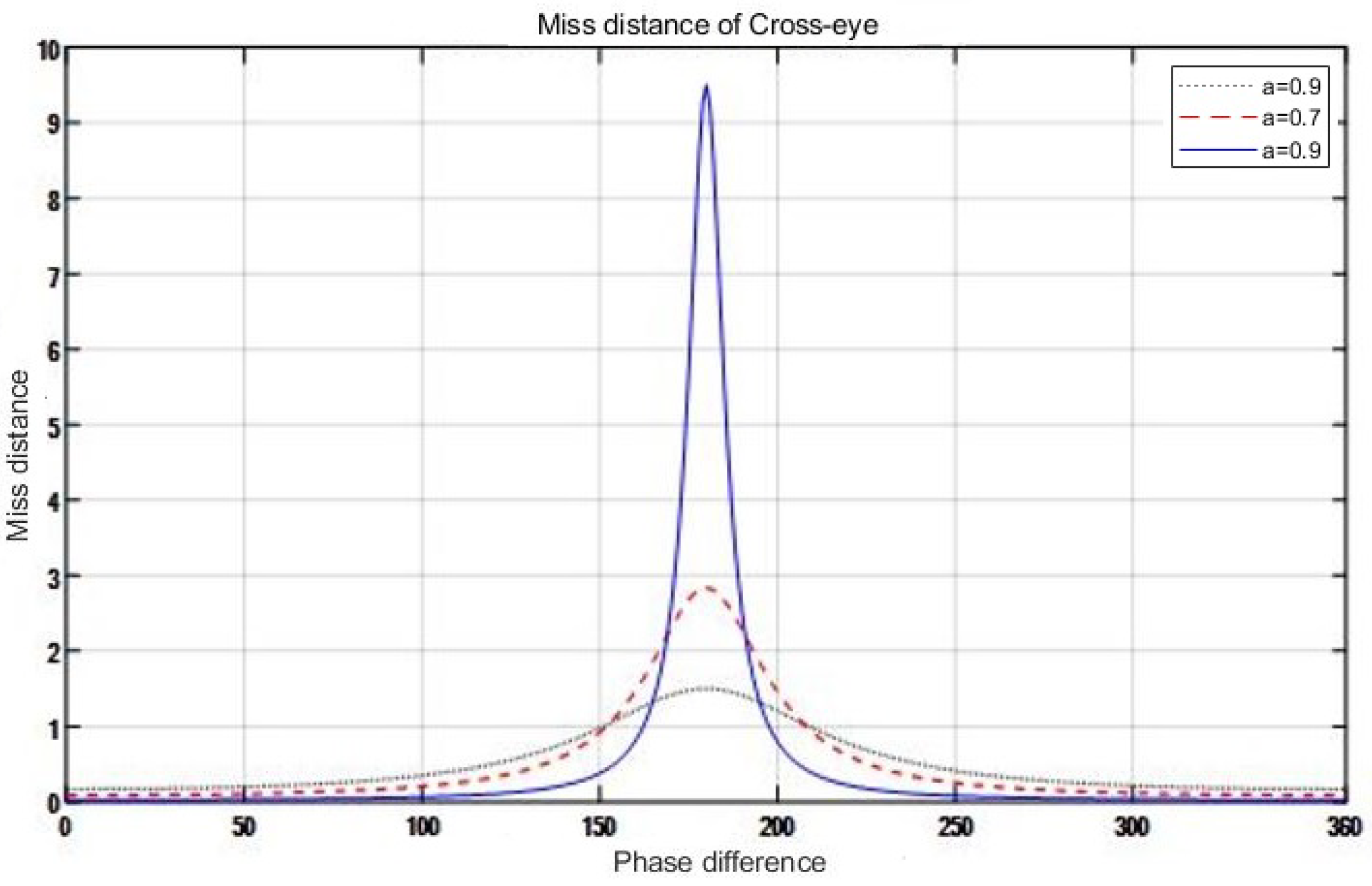
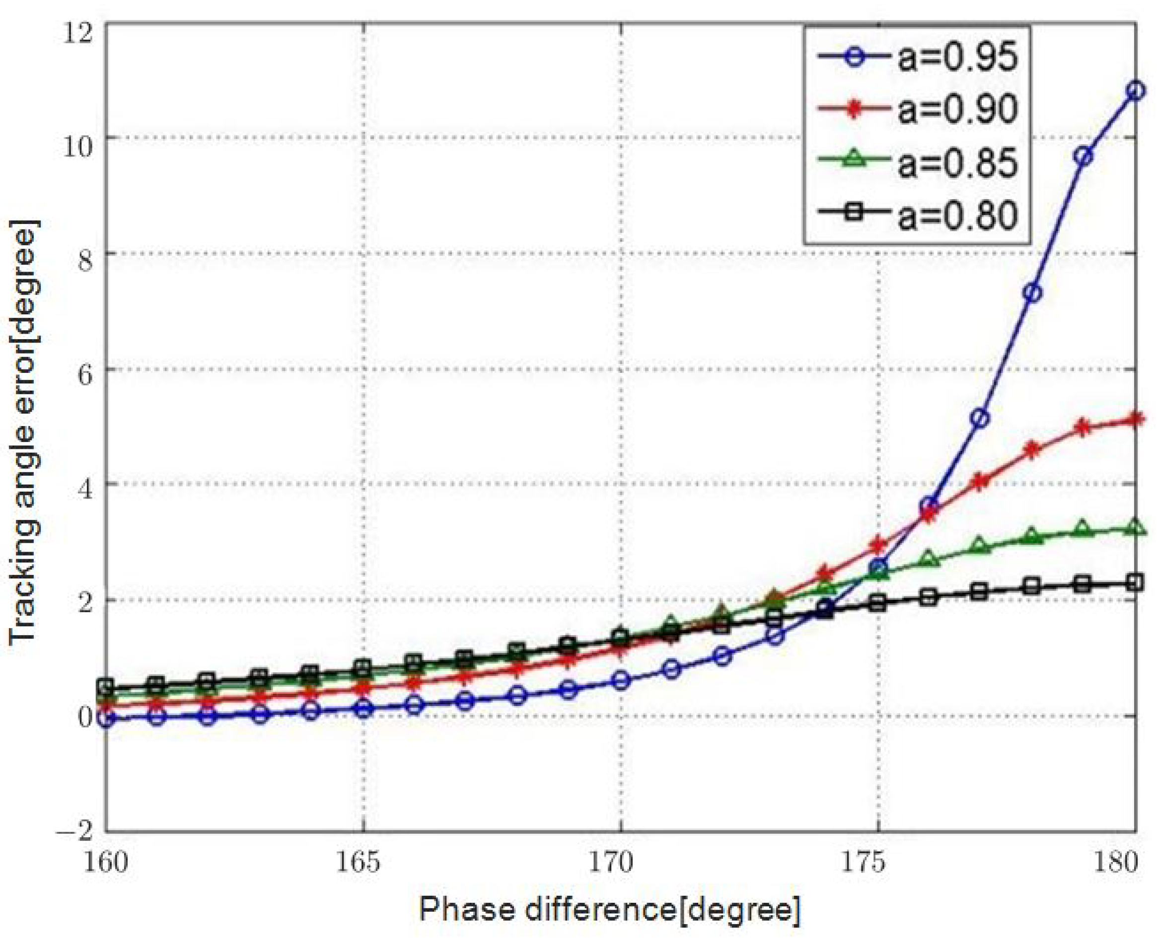
Figure 2 shows that jammer antenna A and jammer antenna B produce a disturbance signal. The cross-eye jamming induces an angular error by recreation the angular error in the jammed radar. The cross-eye jamming effect is sensitive to changing the amplitude ratio and phase difference values of the two jamming signals. Figure 3 shows the miss distance with respect to a, and Figure 4 shows the angle error with respect to amplitude ratio and phase difference. In [15,16,17,18], the authors have made tolerance analysis based on the contour plot. 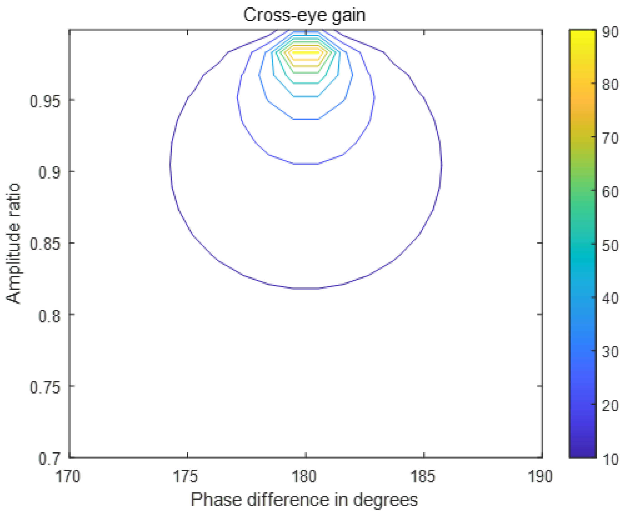In Figure 5, contour plot of the cross-eye gain values, which is similar to the contour plots in [15,16,17,18], are presented. The contour plot in Figure 5 displays how much degradation in cross-eye gain occurs due to a deviation in amplitude ratio and phase difference between two jammer antennas. Accordingly, cross-eye jamming performance is highly dependent on the amplitude ratio and phase difference. Suppose you can model the instability of amplitude ratios and phase differences as zero mean Gaussian random variables:

$$\begin{array}{c}{\delta }_a\sim N(0,{\sigma }_a)\hfill \\ {\delta }_{\varphi }\sim N(0,{\sigma }_{\varphi }),\hfill \end{array}$$

(6)

where ${\sigma }_a$ and ${\sigma }_{\varphi }$ are the standard deviation of amplitude ratio and standard deviation of phase difference, respectively. Therefore, $a_{\mathrm{real}}$ and ${\varphi }_{\mathrm{real}}$, which occur, the perturbation can be written as

$$\begin{array}{c}{a}_{\mathrm{real}}=a_{\mathrm{nominal}}+{\delta }_a\hfill \\ {\varphi }_{\mathrm{real}}={\varphi }_{\mathrm{nominal}}+{\delta }_{\varphi }.\hfill \end{array}$$

(7)

Since cross-eye gain from Equation (3), GC is a function of a and $\varphi$, ${\mathrm{GC}}_{\mathrm{real}}$ and ${\mathrm{GC}}_{\mathrm{nominal}}$ can be expressed in terms of terms $a_{\mathrm{real}}$, ${\varphi }_{\mathrm{real}}$ and $a_{\mathrm{nominal}}$ and ${\varphi }_{\mathrm{nominal}}$:

$$G{C}_{\mathrm{nominal}}(a_{\mathrm{nominal}},{\varphi }_{\mathrm{nominal}})=\frac{1-a_{\mathrm{nominal}}^2}{1+a_{\mathrm{nominal}}^2+2a_{\mathrm{nominal}}cos{\varphi }_{\mathrm{nominal}}}$$

(8)

$$G{C}_{\mathrm{real}}(a_{\mathrm{real}},{\varphi }_{\mathrm{real}})=\frac{1-a_{\mathrm{real}}^2}{1+a_{\mathrm{real}}^2+2a_{\mathrm{real}}cos{\varphi }_{\mathrm{real}}}.$$

(9)

The square of the difference between Equations (8) and (9) can be expressed as

$${\left(G{C}_{\mathrm{real}}-G{C}_{\mathrm{nominal}}\right)}^2={\left(\frac{1-a_{\mathrm{real}}^2}{1+a_{\mathrm{real}}^2+2a_{\mathrm{real}}cos{\varphi }_{\mathrm{real}}}-\frac{1-a_{\mathrm{nominal}}^2}{1+a_{\mathrm{nominal}}^2+2a_{\mathrm{nominal}}cos{\varphi }_{\mathrm{nominal}}}\right)}^2.$$

(10)

Let the MSD denote the expectation of Equation (10):

$$\begin{array}{c}\mathrm{MSD}=\mathrm{E}\left[{\left(G{C}_{\mathrm{real}}-G{C}_{\mathrm{nominal}}\right)}^2\right]\hfill \\ = \mathrm{E}\left[{\left(\frac{1 - a_{\mathrm{real}}^2}{1 + a_{\mathrm{real}}^2 + 2a_{\mathrm{real}}cos{\varphi }_{\mathrm{real}}}-\frac{1 - a_{\mathrm{nominal}}^2}{1 + a_{\mathrm{nominal}}^2 + 2a_{\mathrm{nominal}}cos{\varphi }_{\mathrm{nominal}}}\right)}^2\right].\hfill \end{array}$$

(11)

MSD from the Monte-Carlo simulation can be obtained from:

$$\begin{array}{c}\mathrm{MSD}=\frac{1}{N}{\displaystyle \sum _{i=1}^N}\left({\left(G{C}_{\mathrm{real}}{(a_{\mathrm{real}},{\varphi }_{\mathrm{real}})}_i-G{C}_{\mathrm{nominal}}(a_{\mathrm{nominal}},{\varphi }_{\mathrm{nominal}})\right)}^2\right)\hfill \\ =\mathrm{SimulationE}\left[{\left(G{C}_{\mathrm{real}}{(a_{\mathrm{real}},{\varphi }_{\mathrm{real}})}_i-G{C}_{\mathrm{nominal}}(a_{\mathrm{nominal}},{\varphi }_{\mathrm{nominal}})\right)}^2\right],\hfill \end{array}$$

(12)

where the N is the number of Monte-Carlo repetitions. The simulation-based MSD of the first-order Taylor approximation is given as

$$\mathrm{E}\left[{\left(G{C}_{\mathrm{real}}^{(\mathrm{approxi}=1)}-G{C}_{\mathrm{nominal}}\right)}^2\right]=\mathrm{E}\left[{\left({\alpha }_a(a_{\mathrm{real}}-a_0)+{\alpha }_{\varphi }\left({\varphi }_{\mathrm{real}}-{\varphi }_0\right)\right)}^2\right],$$

(13)

where ${\alpha }_a$ and ${\alpha }_{\varphi }$ are coefficients of the first-order Taylor approximation, respectively. The MSD of the second-order Taylor approximation is given as

$$\begin{array}{c}\mathrm{E}\left[{\left(G{C}_{\mathrm{real}}^{\left(\mathrm{approxi}=2\right)}-G{C}_{\mathrm{nominal}}\right)}^2\right]\hfill \\ =\mathrm{E}\left[{\left(\begin{array}{c}\left(a_a(a_{\mathrm{real}}-a_0)+{\alpha }_{\varphi }\left({\varphi }_{\mathrm{real}}-{\varphi }_0\right)\right)+\\ \left[{\beta }_a{(a_{\mathrm{real}}-a_0)}^2+{\beta }_{a\varphi }\left(a_{\mathrm{real}}-a_0\right)\left({\varphi }_{\mathrm{real}}-{\varphi }_0\right)+{\beta }_{\varphi }{({\varphi }_{\mathrm{real}}-{\varphi }_0)}^2\right]\end{array}\right)}^2\right],\hfill \end{array}$$

(14)

where ${\beta }_a$, ${\beta }_{a\varphi }$ and ${\beta }_{\varphi }$ are coefficients of the second-order Taylor approximation, respectively. The analytic MSD based on the first-order Taylor approximation and the second-order Taylor approximation can be expressed as

$$\mathrm{E}\left[{(\mathrm{GC}}_{\mathrm{real}}^{\mathrm{approxi}=1}-{\mathrm{GC}}_{\mathrm{nominal}}{)}^2\right]={\alpha }_a^2{\sigma }_a^2+{\alpha }_{\varphi }^2{\sigma }_{\varphi }^2$$

(15)

$$\mathrm{E}\left[{(\mathrm{GC}}_{\mathrm{real}}^{\mathrm{approxi}=2}-{\mathrm{GC}}_{\mathrm{nominal}}{)}^2\right]={\alpha }_a^2{\sigma }_a^2+{\alpha }_{\varphi }^2{\sigma }_{\varphi }^2+\frac{3}{4}{\beta }_a^2{\sigma }_a^4+\frac{3}{4}{\beta }_{\varphi }^2{\sigma }_{\varphi }^4+{\beta }_{a\varphi }^2{\sigma }_a^2{\sigma }_{\varphi }^2+\frac{1}{2}{\beta }_a{\beta }_{\varphi }{\sigma }_a^2{\sigma }_{\varphi }^2.$$

(16)

Each coefficient of the first-order Taylor approximation and the second-order Taylor approximation ${\alpha }_a$, ${\alpha }_{\varphi }$, ${\beta }_a$, ${\beta }_{a\varphi }$ and ${\beta }_{\varphi }$ are derived in the Appendix A.

3. Analytic Expression of the MSD Based on Numerical Integration

As shown in Equation (7), $a_{\mathrm{real}}$ and ${\varphi }_{\mathrm{real}}$ are random variables due to perturbation. Because $a_{\mathrm{real}}$ and ${\varphi }_{\mathrm{real}}$ are random variables, the expression in Equation (10) is also a random variable. Thus, the MSD can be calculated by using joint PDF, $f_{a,\varphi }(a,\varphi )$ [19]. The MSD, in terms of the joint PDF, can be written as,

$$\begin{array}{cc}\hfill \mathrm{MSD}& =\mathrm{E}\left[{\left({\mathrm{GC}}_{\mathrm{real}}{-\mathrm{GC}}_{\mathrm{nominal}}\right)}^2\right]\hfill \\ \hfill & ={\int }_{-\infty }^{\infty }{\int }_{-\infty }^{\infty }{\left({\mathrm{GC}}_{\mathrm{real}}{-\mathrm{GC}}_{\mathrm{nominal}}\right)}^2{f}_{a,\varphi }(a,\varphi )dad\varphi ,\hfill \end{array}$$

(17)

where a and $\varphi$ are Gaussian random variables with means $a_0$ and ${\varphi }_0$ and variance ${\sigma }_a$ and ${\sigma }_{\varphi }$, respectively. Therefore, the two variables a and $\varphi$ have Gaussian PDF:

$$f_a\left(a\right)=\frac{1}{{\sigma }_a\sqrt{2\pi }}exp\left(\frac{-{(a-a_0)}^2}{2{\sigma }_a^2}\right)$$

(18)

$$f_{\varphi }\left(\varphi \right)=\frac{1}{{\sigma }_{\varphi }\sqrt{2\pi }}exp\left(\frac{-{(\varphi -{\varphi }_0)}^2}{2{\sigma }_{\varphi }^2}\right).$$

(19)

In general, the joint PDF is not equal to the product of the PDF of each random variable. However, because the two random variables are uncorrelated, joint PDF is identical to the product of the PDF of each random variable:

$$f_{a,\varphi }=f_a\times f_{\varphi }=\frac{1}{{\sigma }_a\sqrt{2\pi }}exp\left(\frac{-{(a-a_0)}^2}{2{\sigma }_a^2}\right)\times \frac{1}{{\sigma }_{\varphi }\sqrt{2\pi }}exp\left(\frac{-{(\varphi -{\varphi }_0)}^2}{2{\sigma }_{\varphi }^2}\right).$$

(20)

Using Equations (17) and (20), numerical integration-based MSD can be written as

$$\begin{array}{c}\mathrm{E}\left[{({\mathrm{GC}}_{\mathrm{real}}-{\mathrm{GC}}_{\mathrm{nominal}})}^2\right]={\int }_{-\infty }^{\infty }{\int }_{-\infty }^{\infty }{(\mathrm{GC}}_{\mathrm{real}}-{\mathrm{GC}}_{\mathrm{nominal}}{)}^2{f}_{a,\varphi }(a,\varphi )dad\varphi \hfill \\ ={\int }_{-\infty }^{\infty }{\int }_{-\infty }^{\infty }{(\mathrm{GC}}_{\mathrm{real}}-{\mathrm{GC}}_{\mathrm{nominal}}{)}^2{f}_a\left(a\right)f_{\varphi }\left(\varphi \right)dad\varphi .\hfill \end{array}$$

(21)

4. Numerical Result of MSD

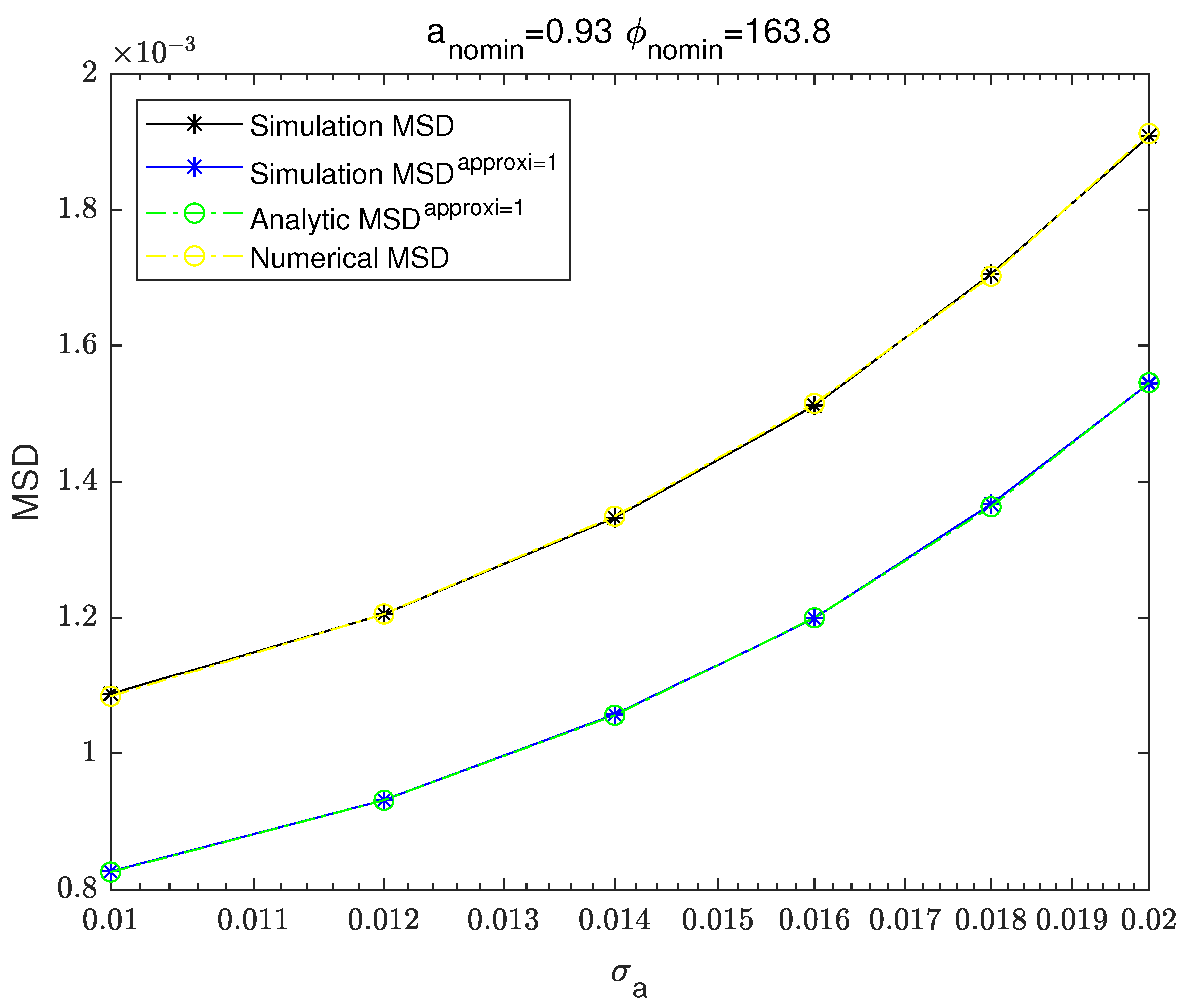
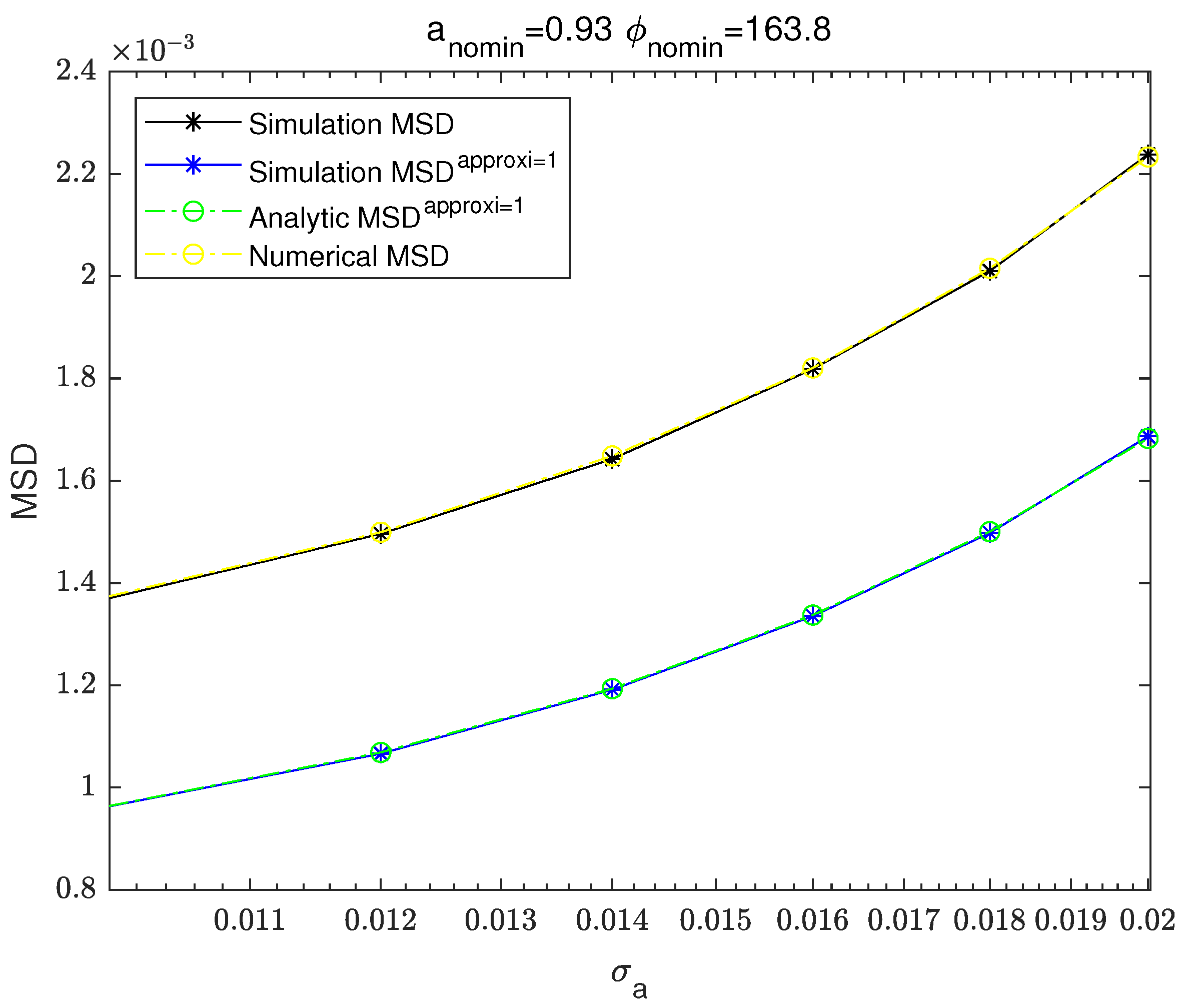
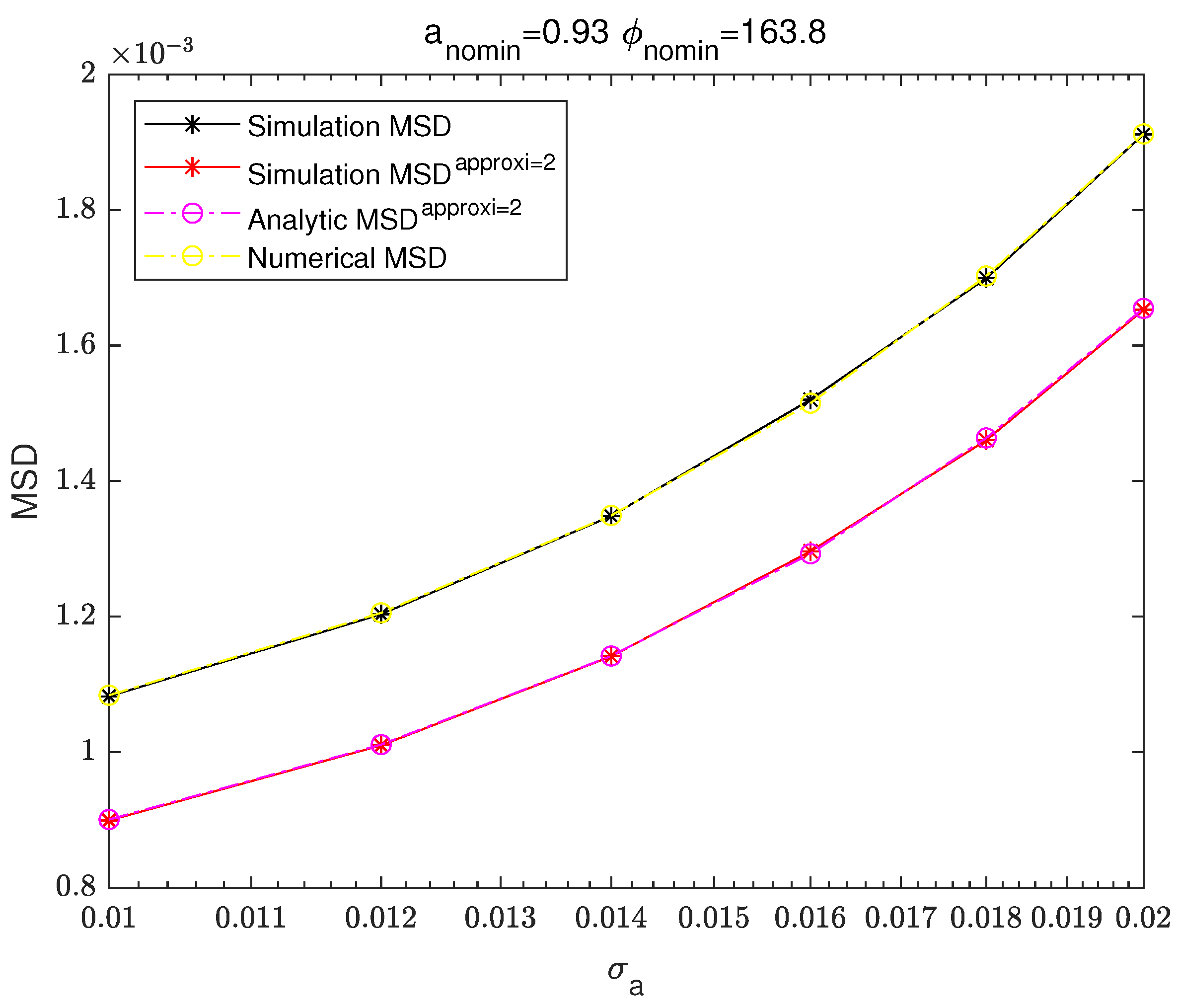
This section deals with the performance analysis of cross-eye jamming using simulation MSD, analytic MSD, and numerical integration-based MSD. To consider various cases, six standard deviations were set for each of ${\sigma }_a$ and ${\sigma }_{\varphi }$ in the simulation. For ${\sigma }_a$, six standard deviations were set from 0.01 to 0.02, and for ${\sigma }_{\varphi }$, standard deviations from 5 to 10 were set.

Table 1. Various standard deviation of cross-eye gain.

Description	Values
Standard deviations of amplitude ratio (${\sigma }_a$)	0.01, 0.012, 0.014, 0.016, 0.018, 0.02
Standard deviations of phase difference (${\sigma }_{\varphi }$)	5, 6, 7, 8, 9, 10 (degrees)

shows each standard deviation values of ${\sigma }_a$ and ${\sigma }_{\varphi }$.

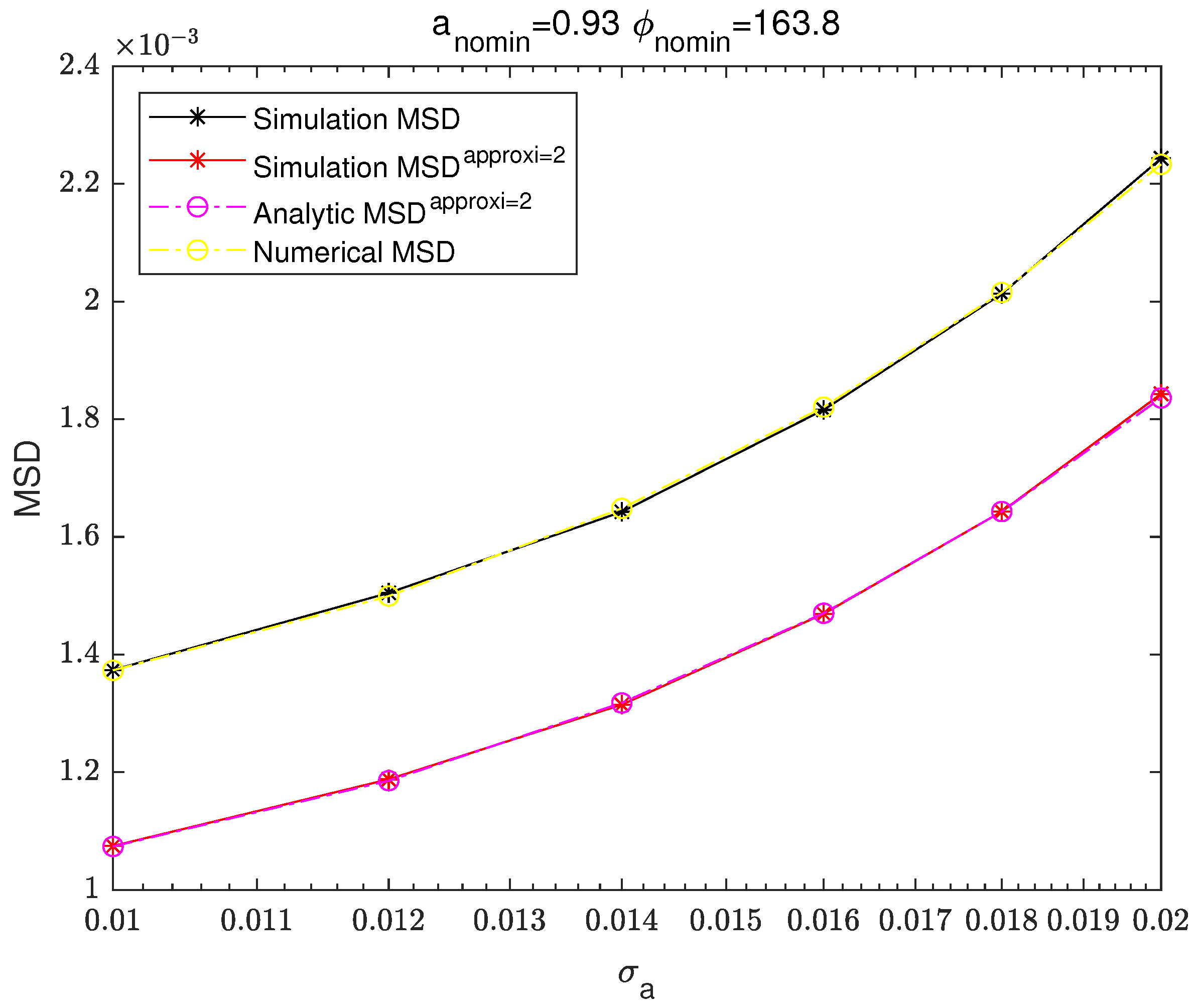
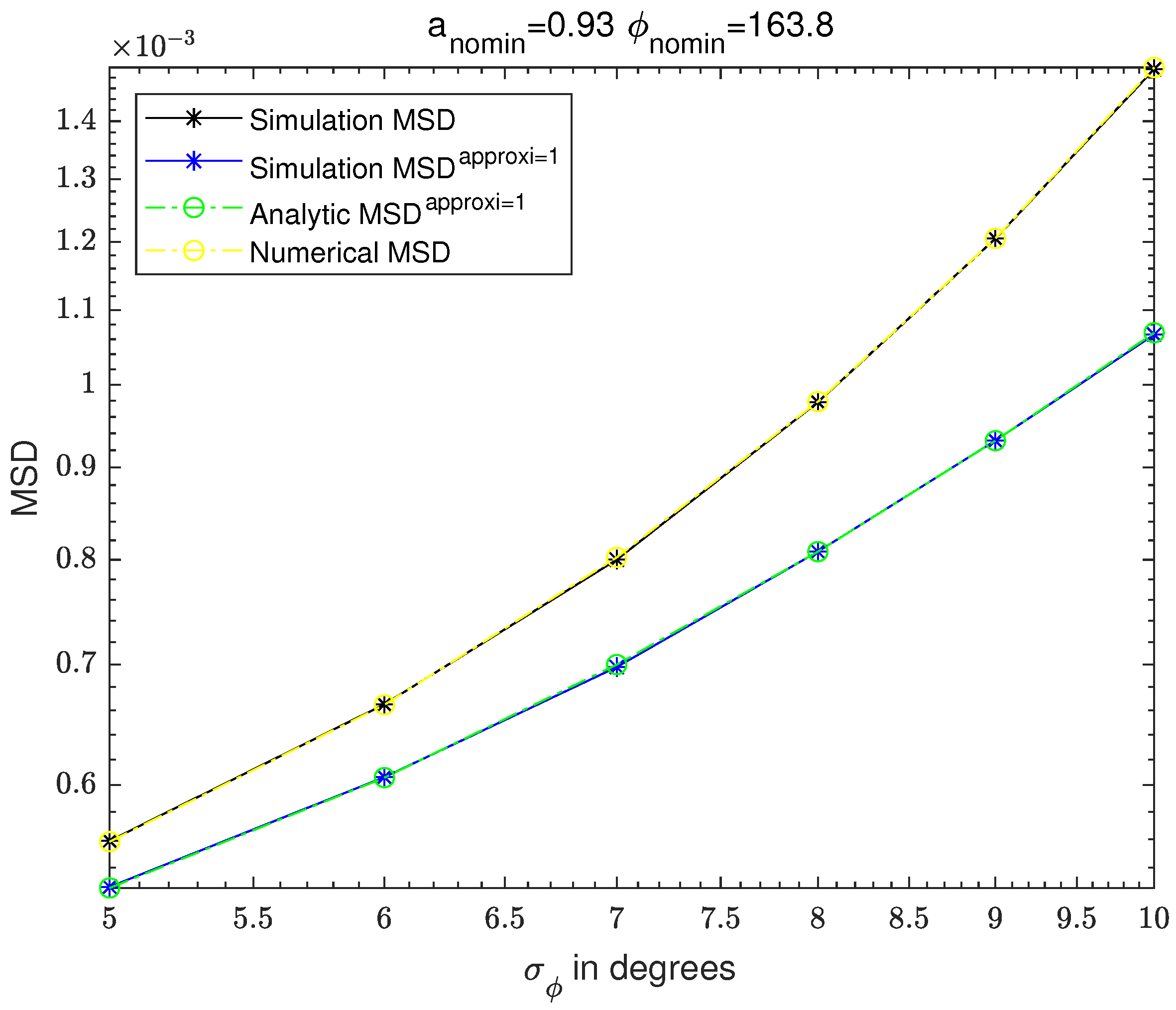
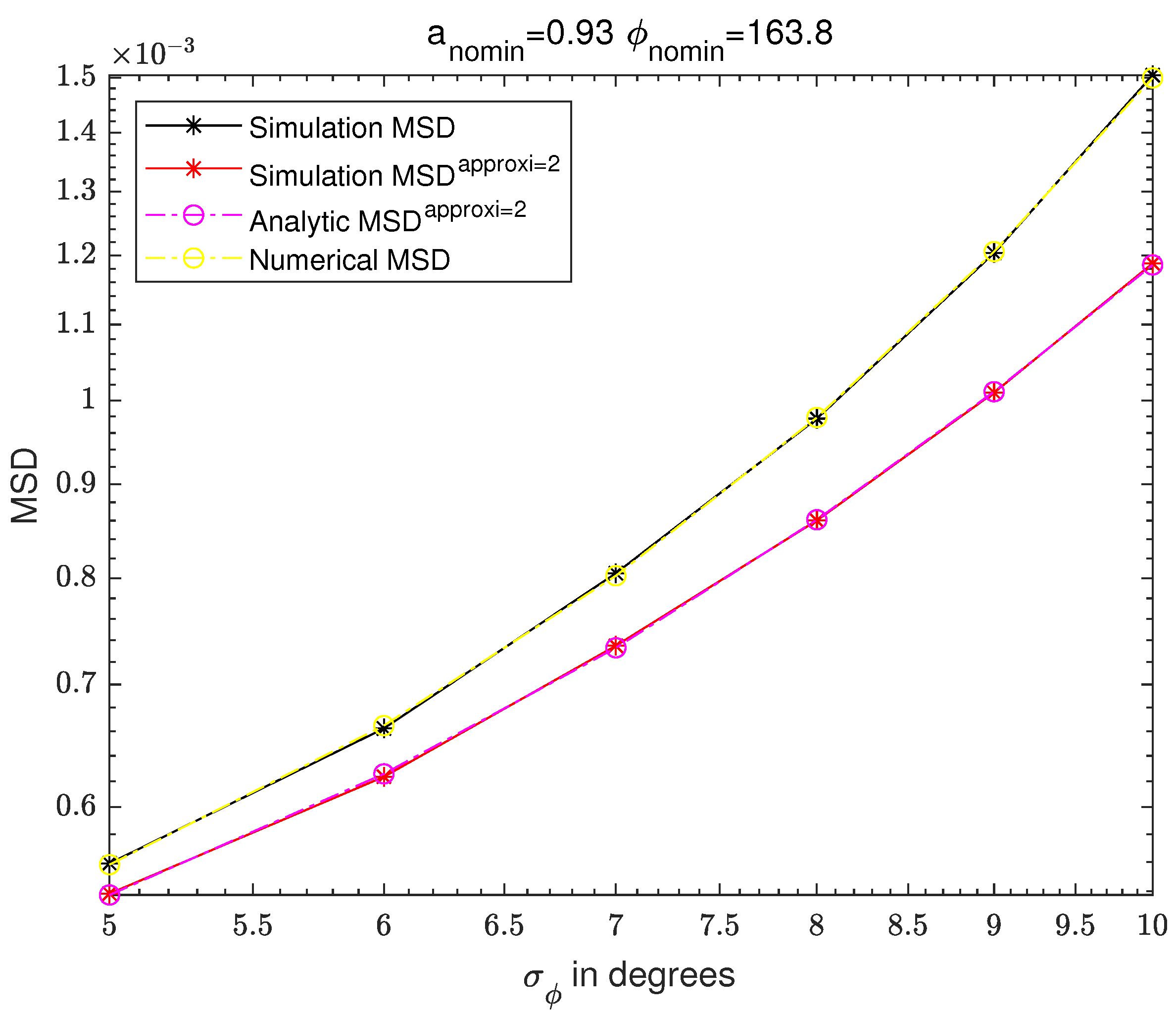
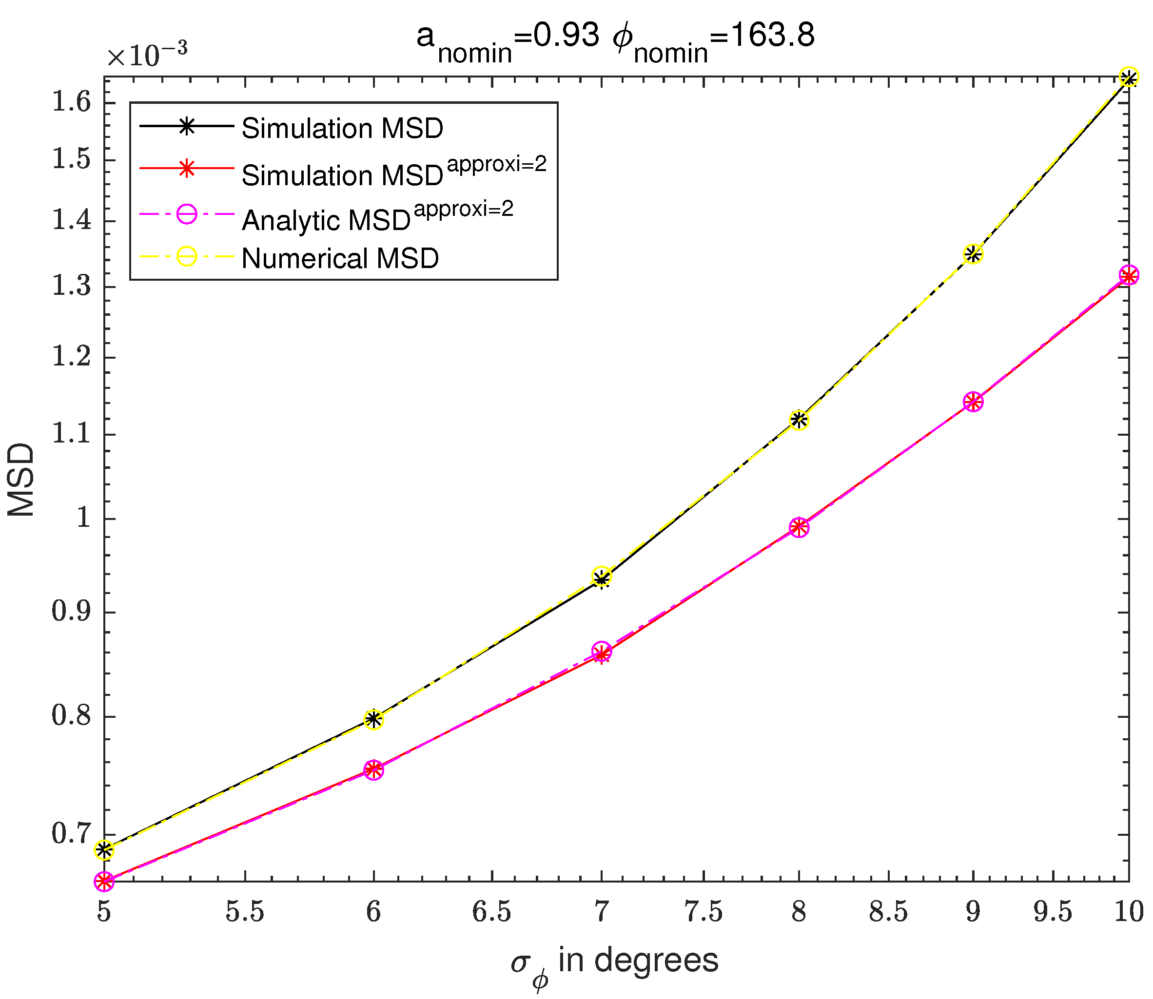
Performance analysis is performed on the amplitude ratio and phase difference, which are random variables including standard deviation. The results of MSD which uses the Monte-Carlo simulation and MSD, which uses the analytic method are compared with the MSD which uses the numerical integral. Figure 6, Figure 7, Figure 8, Figure 9, Figure 10, Figure 11, Figure 12 and Figure 13 show the MSD results in MATLAB when six standard deviations for each of the amplitude ratio and phase difference are used. Figure 6, Figure 7, Figure 8 and Figure 9 are the result graphs of fixing the phase difference’s standard deviation, ${\sigma }_{\varphi }$ and changing the amplitude ratio’s standard deviation, ${\sigma }_a$. Figure 6 and Figure 7 are the graphs of MSD results of the non-approximated simulation-based MSD, the first-order Taylor expansion-based simulation MSD, the first-order Taylor expansion-based analytic MSD and the numerical integration-based MSD. Figure 8 and Figure 9 are the graphs of MSD results of the non-approximated simulation-based MSD, the second-order Taylor expansion-based simulation MSD, the second-order Taylor expansion-based analytic MSD and the numerical integration-based MSD. In contrast, Figure 10, Figure 11, Figure 12 and Figure 13 are the results of fixing ${\sigma }_a$ and changing ${\sigma }_{\varphi }$. The same as Figure 6, Figure 7, Figure 8 and Figure 9, Figure 10 and Figure 11 are the graphs of MSD results of the non-approximated simulation-based MSD, the first-order Taylor expansion-based simulation MSD, the first-order Taylor expansion-based analytic MSD, and the numerical integration-based MSD. Figure 12 and Figure 13 are the graphs of MSD results of the non-approximated simulation-based MSD, the second-order Taylor expansion-based simulation MSD, the second-order Taylor expansion-based analytic MSD, and the numerical integration-based MSD.

The simulation MSD in Figure 6, Figure 7, Figure 8, Figure 9, Figure 10, Figure 11, Figure 12 and Figure 13 are obtained from Equation (11). The first-order Taylor expansion-based simulation MSD and the first-order Taylor expansion-based analytic MSD in Figure 6, Figure 7, Figure 10 and Figure 11 are obtained from Equations (13) and (15), respectively. The second-order Taylor expansion-based simulation MSD and the second-order Taylor expansion-based analytic MSD in Figure 8, Figure 9, Figure 12 and Figure 13 are obtained from Equations (14) and (16), respectively. Finally, numerical integration-based MSD in Figure 6, Figure 7, Figure 8, Figure 9, Figure 10, Figure 11, Figure 12 and Figure 13 is obtained from Equation (21). Simulation-based MSDs are obtained from Equation (12). The first-order Taylor expansion-based simulation MSD shows very good agreement with the first-order Taylor expansion-based analytic MSD. Similarly, the second-order Taylor expansion-based simulation MSD and the second-order Taylor expansion-based analytic MSD show very good agreement. The simulation-based MSD and the numerical integration-based MSD show good agreement.

Table 2. Comparison of operation time.

MSD Method	Operation Time (sec) (Number of Repetitions: 30,000)	Operation Time (sec) (Number of Repetitions: 3,000,000)
Simulation MSD	0.09	8.35
Numerical integration-based MSD	0.03	0.03
Analytic MSD	0.002	0.003

shows the operation time of the Monte-Carlo simulation-based MSD, the analytically-derived MSD and the numerical integration- based MSD. The computational complexity of the Monte-Carlo simulation-based MSD increases with the increase of the number of repetitions in the Monte-Carlo simulation. On the other hand, the computational complexity of the analytic MSD and the numerical integration-based MSD are independent of the number of repetitions since analytic MSD and the numerical integration-based MSD are not obtained from the Monte-Carlo repetitions. The computational complexities of three MSDs are tabulated in Table 2. Comparing the analytic MSD and the numerical integration-based MSD shows the numerical integration-based MSD is more computationally intensive than the analytic MSD. Since the numerical integration-based MSD is implemented via double integration, it is more computationally intensive than analytic-based MSD. The integration-based MSD is associated with the MSD without approximation. On the other hand, the analytic MSD is associated with the first-order Taylor expansion approximated MSD.

5. Conclusions

It can be seen in Equation (3) that the jamming effect of cross-eye changes significantly due to the amplitude ratio and phase difference. That is, the cross-eye gain is the function of amplitude ratio and phase difference. Due to mechanical defects, the amplitude ratio and phase difference can change differently from the nominal values; thus, changing the gain of the cross-eye. Degraded cross-eye gain is denoted by ${\mathrm{GC}}_{\mathrm{real}}$ and the original cross-eye gain is denoted by ${\mathrm{GC}}_{\mathrm{nominal}}$.

${\mathrm{GC}}_{\mathrm{real}}$ is a cross-eye gain obtained from $a_{\mathrm{real}}$ and ${\varphi }_{\mathrm{real}}$, the values of zero mean Gaussian random variables added to the amplitude ratio and phase difference, respectively. MSD is the mean of the squared differences between ${\mathrm{GC}}_{\mathrm{real}}$ and ${\mathrm{GC}}_{\mathrm{nominal}}$. MSD is one of the methods used to measure the accuracy of an estimate. As a way to obtain these MSDs, previous papers introduced the simulation and analytic methods obtained through the first-order Taylor approximation and the second-order Taylor approximation. In the case of the simulation method, a number of repetitions were calculated using the Monte-Carlo method to obtain an MSD. Using this method, it can be shown that computational costs increase as the number of repetitions increases. On the contrary, in the case of the analytic method, it can be confirmed that the calculation cost is independent on the number of repetitions. This confirms that the analytic method has a much lower time cost than the time cost of the simulation. However, cross-eye gain is a nonlinear function shown in a fractional form, it is difficult to develop the mean operation analytically. Thus, the approximations are applied, which leads to poor accuracy. Since approximation has been applied, it can be confirmed that the MSD of the analytical method is close to the MSD of non-approximated simulation method, but not completely matched.

This paper proposed a method for calculating MSD through the numerical integral method. This is the method of calculating the MSD by using numerical integration and a joint PDF. Because a and $\varphi$ are uncorrelated, it can be calculated using each PDF, $f_a$ and $f_{\varphi }$ without using joint PDF, $f_{a,\varphi }$. Equation (21) shows that a double integral is used. Table 1 shows that numerical integration-based MSD time cost is higher than analytic MSD because it uses dual integrals. However, Figure 6 and Figure 13 show the accuracy of numerical integration-based MSD is higher than the accuracy of the analytic MSD. The numerical integration-based MSD is closer to the non-approximation simulation MSD than the analytic MSD. In other words, this means that MSD can be calculated using numerical integration without performing numerous repetitive calculations. The higher the order, the closer the non-approximation MSD, but the higher the order, the higher the complexity and computational time. Therefore, the method calculating an MSD using the numerical integral proposed in this paper can be said to be superior to the analytic method proposed in the previous paper. A quantitative description on performance degradation, due to the imperfect amplitude ratio and phase difference between two jammer antennas, has been presented. More specifically, imperfections in amplitude ratio and phase difference is modeled with zero-mean Gaussian random variables, and the validity of the proposed scheme is shown using numerical results. Future work includes an extension to the non-zero mean Gaussian random variable and an improvement to the accuracy of the numerical integration by adopting more sophisticated numerical integration schemes.

In practical implementation of cross-eye jamming, in the viewpoint of modeling of perturbations in amplitude ratio and phase difference as Gaussian random variables, two extensions can be considered.

At first, in the proposed scheme, the amplitude ratio and phase difference are modeled as zero-mean Gaussian random variables, which are ${\delta }_a$ and ${\delta }_{\varphi }$. In practice, due to systematic bias in jammer system, ${\delta }_a$ and ${\delta }_{\varphi }$ can be non-zero mean Gaussian random variables. The formulation for non-zero mean Gaussian random variable can be derived by extending the formulation propose in this paper.

In addition, ${\delta }_a$ and ${\delta }_{\varphi }$ can be correlated. Since the amplitude ratio and phase difference are obtained from the magnitude and angle of a complex number, they can be correlated. Although taking into account the fact that the amplitude ratio and phase difference can be correlated makes the formulation more complicated, the scheme proposed in this paper, where the amplitude ratio and phase difference are assumed to be uncorrelated, can be extended to the case where the amplitude ratio and phase difference are correlated.