1. Introduction
Time series are generated in many real-world applications [
1] ranging from speech recognition [
2], human activity recognition [
3], and cyber-security [
4] to remote sensing [
5,
6], and experimental techniques (e.g., imaging, scattering or diffraction, and spectroscopy) for advanced research in materials science, physical and chemical sciences, etc. Among them, spectroscopy and diffraction technologies are central to natural sciences and engineering, one of the primary methods to investigate the real world, discover new phenomena and characterize the properties of substances or materials [
7], and is one of the important sources of time series data. These experiments are often time-consuming and sometimes require large, very expensive scientific facilities such as synchrotron light sources or X-ray free-electron lasers (XFELs) [
7]. In these experiments, different kinds of large volume of time-resolved spectra are produced, such as data from Raman spectroscopy, X-ray Diffraction (XRD), X-ray absorption spectroscopy, mass spectroscopy, and infrared spectroscopy, etc. These one-dimensional (1D) spectra time series may have different sources and functions, but their representation forms are the same [
8], and information about their peak positions, intensities, shapes, and areas is crucial.
In scientific research, changes in spectra can indicate changes in the system under investigation. In order to evaluate the experiment status, the measured spectra need to be classified so that each class is assigned to a different state of the system under investigation. The two major spectral changes that we aim to capture in this study are:
The change in intensity distribution (e.g., drop or appearance) of peaks at certain locations, or;
The shift of those in the spectrum.
Recently, spectra analysis based on big data has become a trend [
8]. With developments in machine learning, data-driven machine learning/deep learning (ML/DL) methods have turned out to be very good at discovering intricate structures in high-dimensional data [
9]. The ML/DL-based methods have applied broadly to a set of algorithms and techniques that train systems from raw data rather than a priori models [
10]; thus, useful for research facilities that produce large, multidimensional spectral data.
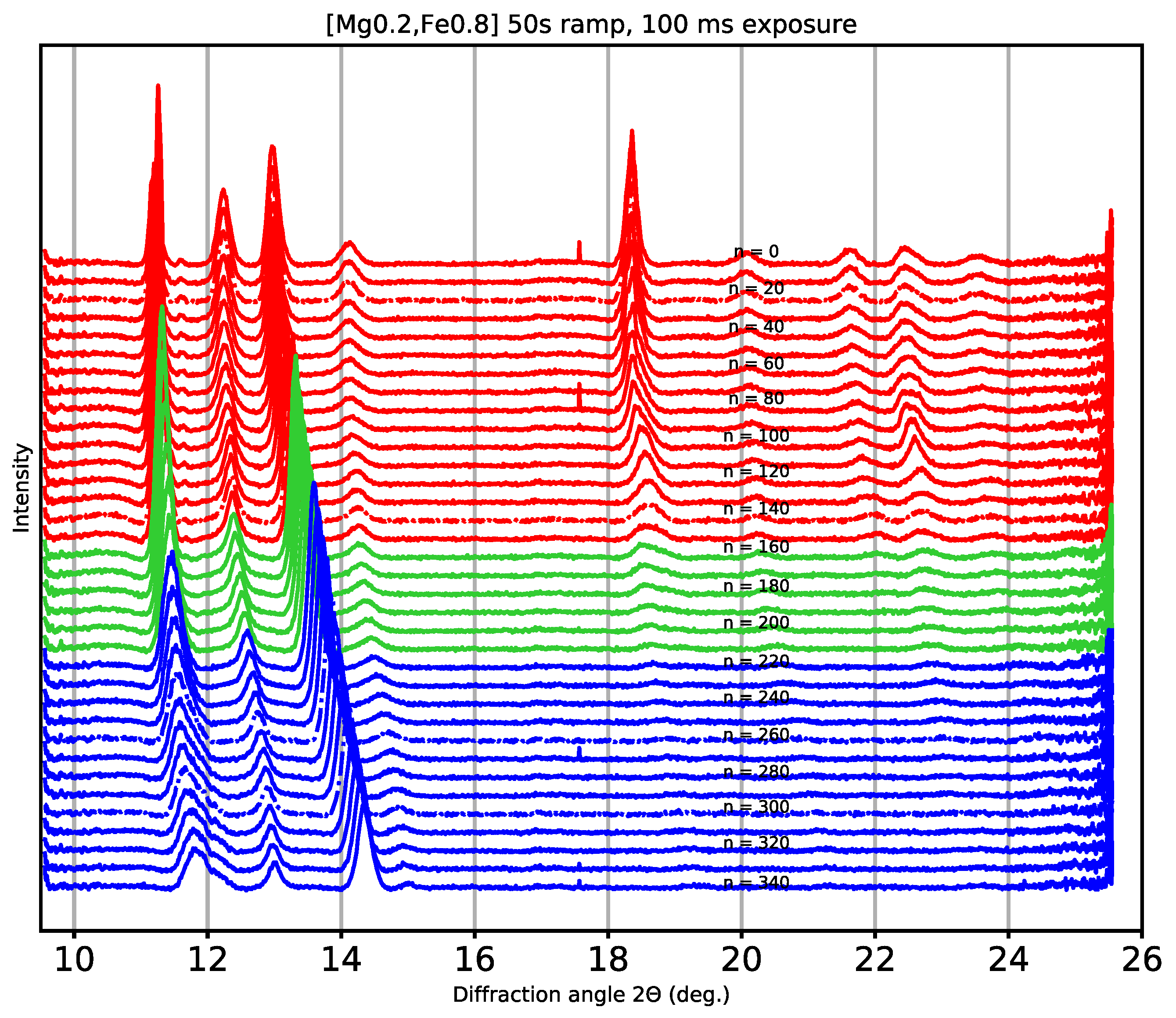
In this study, our goal is to derive an end-to-end statistical model for the application of spectra classification. The spectral data used in this work were collected during an HED experiment, which was obtained through azimuthal integration of raw X-ray diffraction patterns, as shown in
Figure 1. In High Energy Density (HED) [
11] experiments with high-density materials, changes in pressure will cause changes in the spectral peaks (vanishing, shifting, broadening, or splitting); therefore, our diffraction spectra dataset is very representative. The dataset consists of 349 samples, each with 4023 features, and is publicly available (at
https://zenodo.org/record/4424866 accessed on 26 November 2021). To show more clearly how the diffraction changes while the pressure on the sample is changing, we show one for every 10 diffractograms, as displayed in
Figure 1. It can be clearly seen from this figure that the amplitude of spectral peaks changes (increases, decreases, and vanishes) at certain locations, and peaks also shift in a 2θ-angle dimension, or split, or start to broaden [
12]. These changes correspond to modifications of the crystal lattice (e.g., indicating phase changes). Among them, 31 original spectra samples (the 16 marked in red belong to class label 0 and the 15 marked in blue belong to class label 1) are used as a training dataset in supervised methods. We also added 1550 simulated samples for training (by adding sufficiently small random noise, 50 simulated spectral curves can be added to each original diffraction spectrum).
In this work, we provide a standard baseline to exploit several current state-of-the-art deep neural networks for end-to-end 1D spectral time series classification with few labeled samples. We show how DL architectures can be designed and trained efficiently to learn hidden discriminative features from time-resolved spectra in an end-to-end manner. We deal with the spectra classification problem from two different perspectives, either as a general 2D space segmentation problem, or as a common 1D time series classification problem. The explored end-to-end model structures are based on Fully Connected Neural Networks (FCNNs), convolutional neural networks (CNNs), ResNets, Long Short-Term Memory (LSTM), Transformer, and the hybrid architecture of convolution and self-attention.
The performance of these models was compared by reporting their classification confidence, training time, memory consumption, and trainable parameters, and interpretability on HED spectra dataset. Our results show that all classification models can achieve 100% classification confidence, but the models proposed or applied under the 1D time series classification setting are superior. Among them, the LSTM-based model and Transformer-based model consume less time (0.463 s and 0.449 s, respectively) compared with other models. Our proposed convolutional Spatial-Channel-Temporal (SCT) attention model uses 1.269 s and does not take up much memory. Furthermore, a gradient-based feature importance analysis experiment is conducted to exploit the differentiable nature of deep learning models.
It should be noted that, although our classification models are tested on HED diffraction spectra, they are also very suitable for other spectra collected in various diffraction and spectroscopy experiments due to the nice representation of HED spectral data. In addition, since we treat the time-resolved spectra as a standard time series, these models can be easily extended to any other 1D time series classification tasks.
The main contributions of this work can be summarized as follows:
We propose an end-to-end binned FCNN with the automatically capturing weighting factors model in the 2D space segmentation problem setting. The bin-weighting technique can improve classification confidence by minimizing or even eliminating the effects of misclassifications of indistinguishable features, while reducing training time. The structure is particularly suitable for the classification of time series with a large amount of overlap;
We propose a convolutional SCT attention model in the 1D time series classification problem setting. The proposed self-attention architecture can model dependencies across the spatial, channel, and temporal dimensions, which allows it to selectively focus on a few classification-relevant features or observations and suppress indistinguishable features better than others;
In addition to the two models proposed above, we also applied several other state-of-the-art DL models based on FCNN, CNN, ResNets, LSTM, and Transformer in the 1D time series spectra classification problem setting.
Furthermore, we evaluated and compared the classification performance of these DL models on HED spectra data from multiple perspectives. In this way, our work provides a standard baseline for 1D spectral time series classification in an end-to-end manner.
The rest of this study is organized as follows:
Section 2 reviews the recent works related to the commonly state-of-the-art DL mechanisms (FCNN, CNNs, ResNets, RNNs, and Transformer/Self-attention) applied in time series analysis.
Section 3 details the proposed or applied classification models individually. The experiment studies and discussion of results are shown in
Section 4. Finally, the conclusion and future research are provided in
Section 5.
2. Related Work
Many traditional machine learning models, such as k-nearest neighbor (KNN) [
13], Partial Least Squares Discriminant Analysis (PLS-DA) [
14], Extreme Learning Machine (ELM) [
15], and support vector machine (SVM) [
16], have been successfully applied in time series data, as well as time-resolved spectra data in diffraction and spectroscopy techniques. Recently, deep neural networks have received an increasing amount of attention in real-world time series analysis [
17]. A large variety of modeling approaches for univariate and multivariate time series, with deep learning models are recently challenging or replacing the-state-of-the-art in a broad range of tasks such as forecasting, regression, and classification [
18,
19,
20]. The most common established deep learning models in this area are CNN [
21,
22,
23], recurrent neural networks (RNNs) [
18,
24,
25], and attention-based neural networks [
26,
27,
28]. The fully connected architecture is the simplest and most basic architecture, and it is the foundation of all deep learning methods. Usually, it is used in conjunction with other architectures. CNN is based on the shared-weight architecture of the convolution kernels [
29], which can easily capture features. However, since the CNN-based models can only learn local neighborhood features, recently, RNN-based models, attention-based models, and hybrid models are increasingly popular for learning from time series data.
2.1. Tranditional Machine Learning-Based Approach
Numerous traditional machine learning methods have been developed for time series data or specifically spectra data classification [
30]. These traditional methods are unsupervised learning or nonparametric algorithms that do not contain learnable parameters but are more procedural [
31]. Time series data, especially time-resolved spectra data, commonly has a high dimensionality, and it is very common for the number of input variables (features) to be greater than the number of samples. These algorithms can effectively identify underlying patterns or key descriptors in spectra data [
31]. For instance, principle component analysis (PCA) is usually used as a dimensionality reduction by using an orthogonal transformation to convert original data into a set uncorrelated variables of higher space; k-means clustering, is widely used for exploratory data analysis, applied to data clustering; random forest, which is an ensemble learning method based on multiple decision trees, always results in the convergence of generalization error [
32], and can be used for classification and regression. The authors of [
33] presented a novel method called nearest clusters based PLS-DA (NCPLS-DA) to analyze the classification of spectral data. The proposed method can effectively address the multimodality and nonlinearity issues. The work [
30] proposed a framework for spectra data classification using the kernel extreme learning machine (KELM). They used PCA as spectra preprocessing and dimensionality reduction, and then applied the kernel extreme learning machine for classification. One of the most relevant studies to our work [
34] presented the Phase-Mapper, based on convolutive nonnegative matrix factorization (NMF), which can effectively solve the multi-phase identification problem in the context of x-ray diffraction (XRD). Even though these traditional ML classification methods are widely recognized, there are still some questions. For example, they usually require the pretreatment of data and rely heavily on preprocessing such as the PCA, which makes end-to-end work difficult.
2.2. Convolutional-Based Approach
Convolutional neural network (CNN) [
21,
22,
23,
27] is one of the most commonly established deep learning models in time series data analysis. It can easily and effectively capture features in multi-scale by different convolution kernels and pooling operations. Many powerful CNN-based models have been proposed and have achieved great success. Among them, the authors of [
29] applied a combination of 1D and 2D CNN to multisource multitemporal satellite imagery for crop classification. It explored the features across spectral and spatial dimensions but did not consider temporal information. Meanwhile, Temporal Convolutional Neural Network (TempCNN) [
35] where convolutions are applied in temporal dimension, is also well-explored. In [
35], an exhaustive study of one-dimensional TempCNNs for the Classification of Satellite Image Time Series was conducted, their experimental results show that TempCNNs are superior to RNNs in terms of SITS classification. The Conv1D-based classification model designed in [
36] further proved the effectiveness of TempCNNs in processing the temporal dimension of time series classification. Residual Networks (ResNets) [
37] are another common backbone architecture in computer vision and are also adapted to time series classification [
5,
27,
38], the residual connections or shortcut [
37] in the model numerically add higher-level features to the forward propagated representation [
5] and help to propagate the gradient back through the network, so very deep models can be trained [
37]. Based on ResNet, Multiscale architectures [
38] can process time series at multiple scales and achieve feature fusion by concentrating each stream. The Fully Convolutional Network (FCN) [
39] which can yield a fixed-length feature for classification has also been well-exploited and has been shown to achieve the state-of-the-art performance for end-to-end time series classification [
17]. In addition, dilated convolutions are also widely used to improve the feature resolution [
40,
41]. In scientific research, the enormous potential of CNN-based methods has also been demonstrated in spectroscopy and diffraction technologies, including bacterial classification from Raman spectra [
42], classification of edible oils using low field nuclear magnetic resonance [
43], and spectra classification in the field of Neutron and X-ray Diffraction (XRD) [
31,
44]. For example, Oviedo et al. [
44] represented their XRD pattern as time series and applied a CNN-based model to achieve the rapid prediction and classification of crystallographic dimensionality and space group.
Although great progress has been achieved through CNN-based networks, there are still some limitations, namely the inability of leveraging the relationship between features in a global view. To utilize both spatial and temporal features from time series, combinations of convolutional operation and recurrent operation [
17,
45] or attention mechanism [
46,
47] were explored and comprehensively compared.
2.3. Recurrent-Based Approach
For time series data processing, two variants of the RNN models, Long Short-Term Memory (LSTM) [
48], Gated Recurrent Unit (GRU) [
49], in particular, can effectively capture temporal dependencies, thus can work efficiently on various complex time series processing tasks, such as prediction, recognition, and classification [
18,
24,
25,
50,
51,
52]. For example, Lipton et al. [
25] showed the ability of LSTMs to recognize patterns in multivariate time series of clinical measurements. In the meantime, RNN-based architecture is also used in combination with the CNN-based module to construct a hybrid convolutional-recurrent neural architecture that can automatically extract features and capture their short-term and long-term dependencies at the same time [
17,
18,
21]. Lai et al. [
18] developed a Long- and Short-term Time-series network (LSTNet) framework for multivariate time series forecasting. The method combines the strengths of CNN and RNN, and can effectively extract short-term local dependency patterns and long-term patterns in data at the same time. In addition, they exploited an attention mechanism to alleviate the issue of nonseasonal time series prediction. Karim et al. [
17] proposed LSTM FCN and ALSTM-FCN deep learning models for end-to-end time series classification, which are enhancements of a Fully Convolutional Network (FCN) with LSTM sub-module or attention LSTM sub-module. Although the enhanced models can significantly improve classification performance, the limitation is that it is designed for univariate time series. In 2019, the authors of [
45] subsequently introduced squeeze-and-excitation block to augment the FCN block in the existing LSTM-FCN and ALSTM-FCN models, which can capture the contexture information and channel-wise dependencies, so that the model can be used for multivariate time series classification. Interdonato et al. [
52] proposed an end-to-end DuPLO deep learning architecture for the analysis of Satellite Image Time Series data. It is also a combination of both CNNs and GRUs models, which can exploit feature information from different points of view, and then produce more diverse and complete information representations for classification tasks [
52].
RNN-based models have also been applied to spectra classification in spectroscopy. For example, in [
53], Dandıl et al. detected the pseudo-brain tumors via stacked LSTM neural network with Magnetic resonance spectroscopy (MRS) data, achieving high-precision binary classification of brain tumors and normal brain tissue. In [
54], the RNN models were built to analyze Raman spectra to classify blood species. However, the application of RNNs to time-resolved neutron or x-ray scattering experiments is still scarce [
31].
2.4. Attention-Based Approach
Very recently, inspired by the Transformer scaling successes in NLP [
26], researches have also successfully developed their Transformer-based or attention-based models in the tasks of time series analyses such as video understanding [
28], forecasting of multivariate time series data [
51], satellite image time series classification [
21], hyperspectral image (HSI) classification [
55], and other time series classification tasks [
20,
27]. Instead of processing data in an ordered sequence manner, the Transformer model processes an entire sequence of data and uses self-attention mechanisms to learn dependencies in the sequence [
56]. Ma et al. [
57] first proposed a novel approach called Cross-Dimensional Self-Attention (CDSA) for the multivariate, geo-tagged time series data imputation task. The CDSA model can jointly capture the self-attention across multiple dimensions (time, location, measurement), yet in an order-independent way [
57]. Garnot et al. [
21] proposed a spatio-temporal classifier for automatic classification of satellite image time series, in which a Pixel-Set Encoder is used to extract spatial features, and a self-attention-based temporal encoder is used to extract temporal features. This architecture has achieved significant improvements in accuracy, time, and memory consumption. Rußwurm et al. [
5] explored and compared several commonly used state-of-the-art deep learning mechanisms on preprocessed and raw satellite data, such as convolution, recurrence, and self-attention, for crop type identification. They pointed out that preprocessing still improved the classification performance of all models they applied, while the choice of model was less crucial [
5]. In addition, their experiments showed that self-attention and RNNs outperform CNNs on raw satellite time series. They investigated this further though a gradient-based feature importance analysis and qualitatively showed that self-attention mechanism can focus selectively on a few classification-relevant observations. Their work focuses on applying, comparing, and analyzing existing models, rather than proposing new architectures or models. Although attention-based DL models are increasingly popular in various time series classification tasks, its application in X-ray spectroscopy and diffraction techniques is still limited.
Similar to [
5], our work also applies and compares the state-of-the-art 1D-CNN, RNN (LSTM), and self-attention mechanism. We focus on proposing new architectures for spectral time series classification, and deal with this problem from two different perspectives, either as a 2D space segmentation problem (end-to-end binned FCNN with the automatically capturing weighting factors model, as described in
Section 3.1), or as a general 1D time series classification problem (e.g., convolutional SCT attention model, as described in
Section 3.2). Moreover, their models are designed for crop type classification, while our models focus on the application of spectral data classification. In our previous work [
12], we used PCA as data preprocessing for dimensionality reduction, and applied unsupervised spectra clustering, and supervised LSTM-based and Transorformer-based models for HED diffraction spectra classification. These models are not end-to-end solutions, nor can they take advantage of temporal dependencies. Another work by Fawaz et al. [
1] conducted a detailed and comprehensive study of the most recent state-of-the-art performance of deep learning algorithms for time series classification. In their review work, they detailed several deep learning models based on Multi-layer perceptrons, CNN, ResNet, Encoder [
58], and Time-CNN [
59]. They trained and tested these models across multiple time series datasets including univariate and multivariate, and analyzed the corresponding advantages and drawbacks. They did not include and compare the state-of-the-art Transformer-based or self-attention-based model, and RNN-based models (such as LSTM or GRU), which are currently the most state-of-the-art structures. The only attention calculation they involved is in the Encoder model, and it is soft attention. Different from [
1], our work implements these two methods for spectra times series classification, and also focuses on the attention-based architecture to leverage information from different dimensions to extract more complete and powerful feature representations.
3. Data-Driven End-to-End Neural Network Methods
In this section, we describe in detail the DL classification models we proposed or applied in different problem settings. The reasons behind our design or choice of these end-to-end methods are also explained. The first model is proposed in the setting of 2D space segmentation, which applies the bin-weighting technique to suppress the effects of misclassifications of indistinguishable features in overlapping regions. The second model is proposed under the setting of 1D time series classification. It is a hybrid model of CNN and self-attention architecture, where self-attention is calculated across spatial, channel, and temporal dimensions. The remaining models in the third part of this section are other state-of-the-art solutions that we applied to 1D spectra classification in the 1D time series classification problem setting, based on FCNN, CNN, Resnet, LSTM, and Transformer.
3.1. End-to-End Binned FCNN with the Automatically Capturing Weighting Factors Model
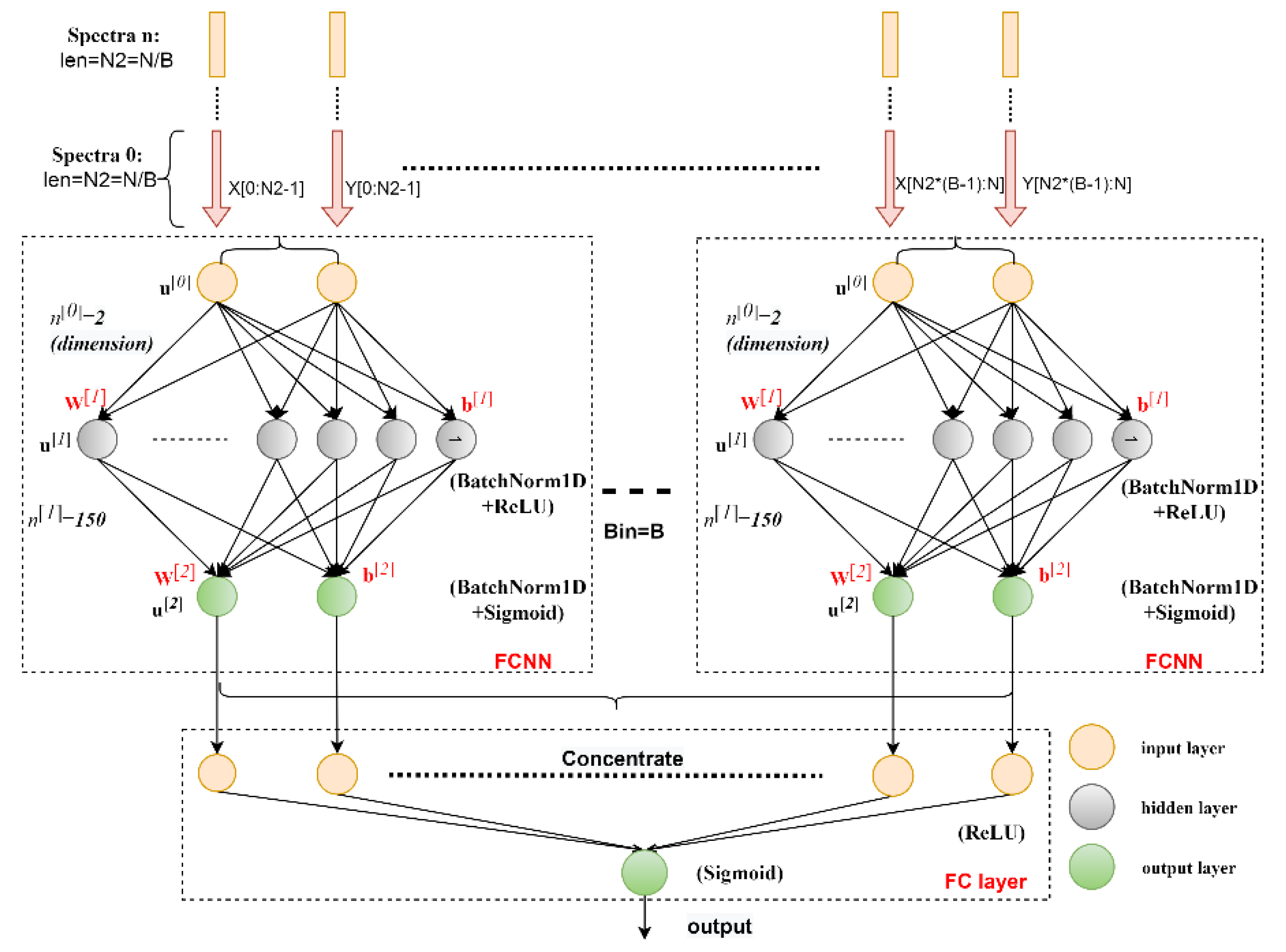
In this model, the spectra classification task is regarded as a general two-dimensional (2D) space segmentation problem. The 2D mentioned here means that instead of inputting a single variable, the values of the two coordinates of each feature point are input into the neural network model, and the model is taught which class label this point belongs to. The model aims to automatically prominent features with high separability and suppress features with low separability. Obviously, the separability of the spectra in the overlapping regions is very low, which is indicated by the low classification accuracy and reliability. Taking this into account, we divided the spectral data into several bins of the same size and used a two-layer Fully Connected Neural Network (FCNN) with the same structure to learn representative features in each local bin. The learned features are then fed into another fully connected (FC) layer to learn the local believability weighting factors of different bins, which are used to classify any spectral time series.
The structure of the end-to-end binned FCNN with the automatically capturing weighting factors model is shown in
Figure 2, which is an extension of our previous work [
60]. In this model, each FCNN sub-module consists of two fully connected layers (FCs), with each one followed by a batch normalization operation and a rectified linear unit (ReLU) [
61] or sigmoid activation function [
62] to speed up the training process and avoid overfitting. The input layer has 2 input neurons, corresponding to the dimensions (two coordinates) of the input spectra, the hidden layer has 150 neurons, and the output layer has 2 output neurons. Then, the output of these FCNN sub-modules is concentrated and fully connected to the final output neuron. The weighting factors learned by the last FC layer can assign different weights to different bins, thereby reducing the influence of the interval of indistinguishable features, and making the features in bins with high separability and reliability more dominant, which can better extract features and learn patterns from the input data. The reason why the sigmoid function is used instead of ReLU after the second FC layer is that we treat each FCNN sub-module as a complete classification model in each bin, so the function of the last FC layer is mainly to assign an overall classification influence weight to each bin.
When the number of bins is 1, the model becomes a standard three-layer FCNN, also known as a multi-layer perceptron (MLP). In
Section 4, we experimentally demonstrate the advantages of the bin-weighting technique in terms of classification confidence, required training epochs, and training time.
3.2. Convolutional SCT Attention Network
More generally, the spectral data can be regarded as typical 1D time series data. In this setting, several other classification models can be explored. As a powerful network, CNN can learn features from different scales, but unfortunately, it cannot capture feature dependencies in a global view. To solve this problem, some methods involving attention mechanisms have been proposed [
5,
26,
46,
47,
63], which investigate attention across single or multiple dimensions. Inspired by the study [
26,
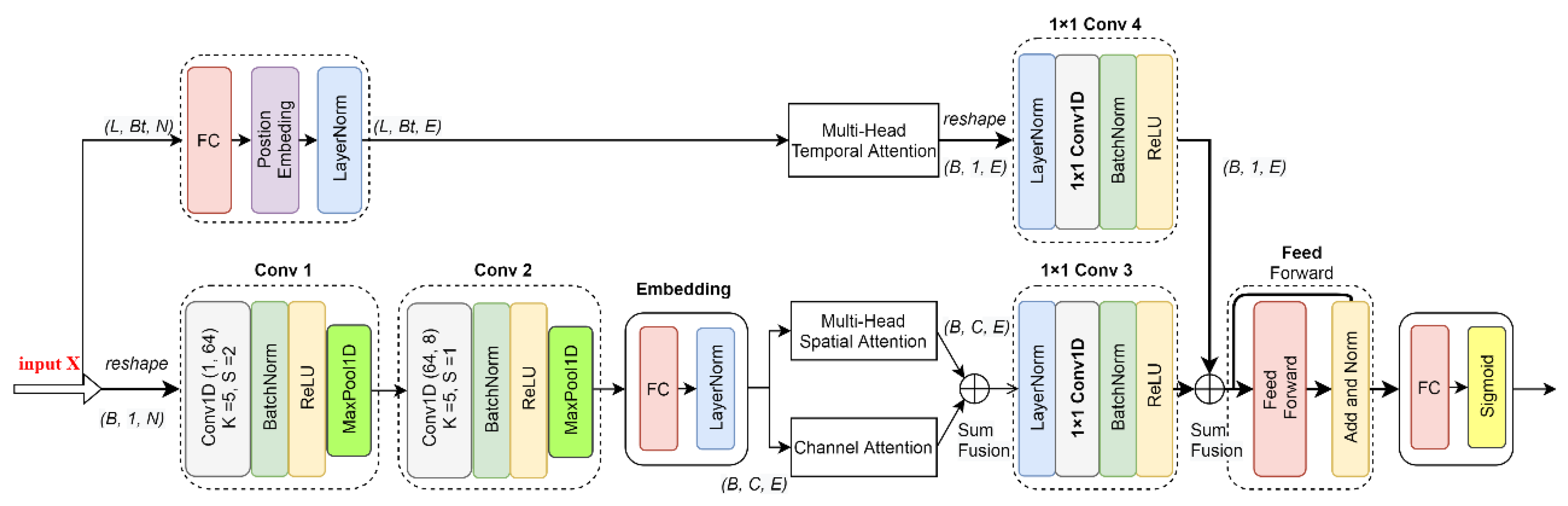
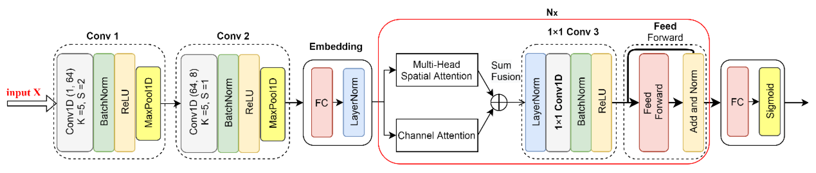
63], we designed a lightweight convolutional Spatial-Channel-Temporal (SCT) attention network for the application of time-resolved spectra classification, as shown in
Figure 3.
The framework consists of two branches. The upper branch models the global contextual information in the temporal dimension. The lower branch model captures global dependencies across the channel and temporal dimensions. These two branches are then aggregated together to better represent features. Finally, a Feed Forward module and a FC module are applied for the classification task.
3.2.1. Spatial Attention Module and Channel Attention Module
In the lower branch (also the main branch), two convolutional modules Conv 1 and Conv 2 are first applied to extract local features. They have the same structure as the convolution modules in the CNN model, consisting of a 1D convolutional layer, a BatchNorm1d function, a ReLU activation function, and a MaxPool1D operation. The number of filters of the convolutional layer in Conv 1 and Conv 2 is 64 and 8, respectively, the kernel size is 5 and 5, respectively, and the step size is 2 and 1, respectively. The size of the kernel and the stride of the MaxPool1D operation in these two modules are 2. In order to facilitate the follow-up Multi-Head attention operation, the embedding module is added, which contains a fully connected layer, and a 1D layer normalization operation. It produces an output of dimension .
We denote the input shape of this branch as of , where B is the batch size, is the number of channels, equal to 1 in the input, and is the number of features. After embedding the module, the output is of shape , where E is the number of embedded features, .
In this branch, two parallel attention modules are applied, a spatial attention module and a channel attention module. The spatial attention module is designed to model the spatial dependencies between any two local features. The channel attention module is designed to capture the global interdependencies over any two channel maps introduced by the Conv 1 and Conv 2 module. These two attention modules are performed concurrently and simply fused through element-wise addition.
Specifically, the Multi-Head spatial attention module is designed based on [
26]. If the batch dimension is not considered, we can denote the input of the attention module as
, then Multi-Head spatial attention can be expressed as:
where
,
and
. In this work, we employ
parallel attention heads, with
. At last, a residual connection is added, which can be expressed as:
Here, the query, key, value used to calculate Multi-Head attention are obtained directly from without transformation. The spatial attention matrix . According to Equation (3), the obtained spatial feature is a weighted sum of all local features and original features. It achieved global spatial interdependencies by selectively aggregating spatial contexts according to the spatial attention matrix .
The channel attention module is designed based on [
63], and we extend their method from three-dimensional image processing to a 1D time series analysis. The channel attention matrix is calculated through
which can be described as:
where
, and
, it models the dependencies or similarity between any two channels.
These two attention modules are fused together through element-wise addition. A convolution module 1 × 1 conv3 is performed after the parallel attention modules, which consists of a layer of normalization operation, 1 × 1 convolution, batch normalization, and a ReLU function. It is used for channel-wise pooling and dimensionality reduction. After this module, the output shape is (B, 1, E).
3.2.2. Temporal Attention Module
The temporal attention module is illustrated in the upper branch of
Figure 3. It is introduced to model the interconnections of any two spectral time series. Before applying the Multi-Head temporal attention, the input spectra are first fed into an FC embedding module and a position embedding module. Its dimension of output
is set to
, which is the same as the output dimension of the embedding module in the spatial and channel attention path.
The shape of input in the upper branch is
, where
is the sequence length, and
is the batch size in the temporal attention branch. Similar to the Transformer-based model, the input sequence length
is set to 31 during training and 349 during testing, which corresponds to the number of original training examples and the total number of spectral curves in the test dataset. The Multi-Head temporal attention is expressed as:
where
,
and
. In this work, we employ
parallel temporal attention heads. At last, a residual connection is added, which can be expressed as:
The temporal query, key, value used to calculate the temporal Multi-Head attention are obtained from the . The temporal attention matrix . According to Equation (7), in our application, the shape of the obtained temporal feature map is (31, 31) during training, and (349, 349) during testing.
After calculating Multi-Head temporal attention, we reshape the output into the shape of (B, 1, E), and apply a 1 × 1 Conv 4 module. The convolutional layer in the 1 × 1 Conv 4 module serves as a scaling function for embedded temporal attention features, instead of changing the depth of feature maps as in the 1 × 1 Conv 3 module.
The temporal features with attention are also simply fused with the other two attention modules through element-wise addition. By applying the 1 × 1 convolution modules, the features in these three attention modules can be easily fused.
After that, a residual feed forward module with the same structure as in [
26] is applied to further capture the features. Finally, an FC layer with the sigmoid activation function is applied to the classification task.
In fact, the attention modules designed in this architecture can also be used individually or concurrently in combination with any other models applied in our work (i.e., FC, ResNet, LSTM, et al.). If we only model connections across spatial and channel dimensions, we can obtain another architecture, named the convolutional SC attention model, which discards the upper temporal attention branch, as illustrated in
Appendix A.
3.3. Other State-of-the-Art Deep Learning Approaches
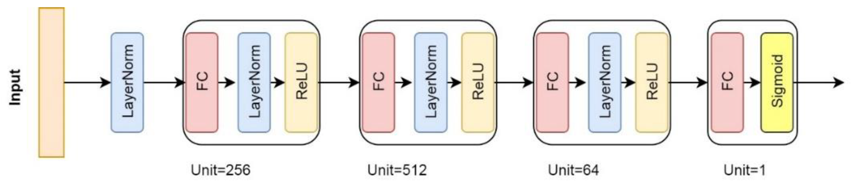
3.3.1. D Multi-Layer Fully Connected Neural Network (1D FCNN) Model
In this solution, we apply a 1D multi-layer Fully Connected Neural Network (1D FCNN) model for time series spectra classification, which has the most interpretable structure, as shown in
Figure A2. It is a basic MLP by stacking four fully connected layers and is designed by following two design rules: (i) using Layer Normalization operation and dropout [
64] (optionally) after each FC layer to speed up training and improve the generalization capability; and (ii) applying ReLU activation function to prevent saturation of the gradient [
27]. See
Appendix B for more details.
3.3.2. Convolutional Neural Network (CNN) Solution
The key feature of a convolution operation is weight sharing, which makes it very suitable for automatically and adaptively learning hierarchies of features [
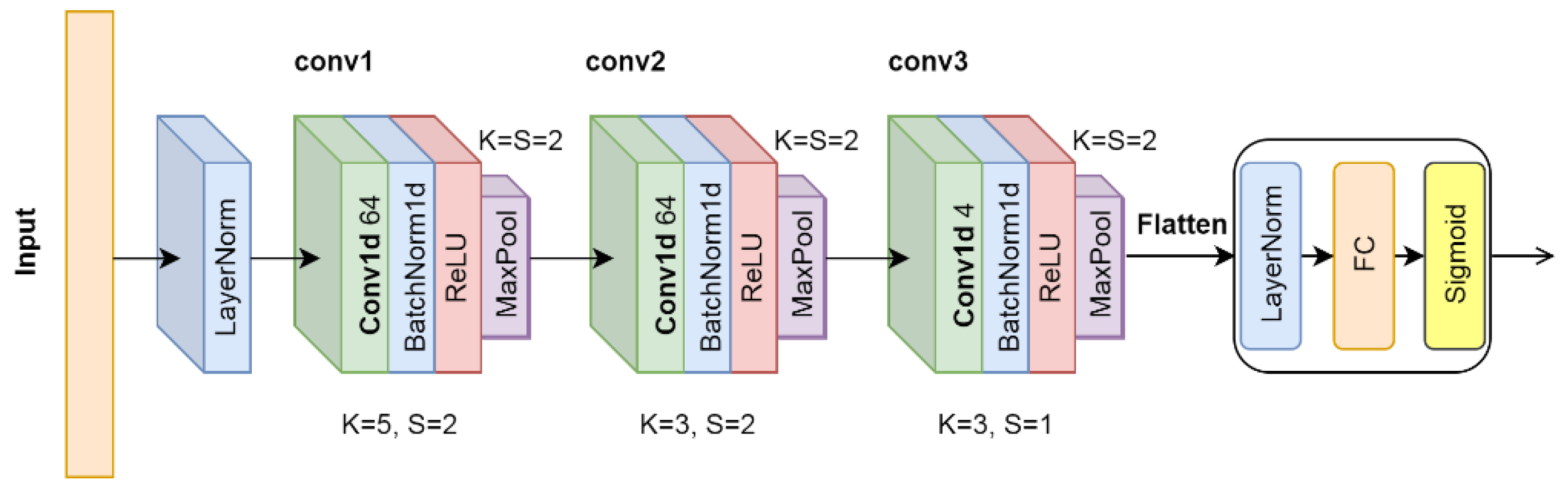
29]. Based on this, we design a CNN-based model with reasonable layers of different sizes of kernels. This model is powerful enough for the spectral time series classification in our application. The architecture of the CNN model is shown in
Figure A3. It is mainly composed of three sequential convolutional modules and one FC module, which are used as the feature extractor and classifier respectively. More details can be found in
Appendix C.
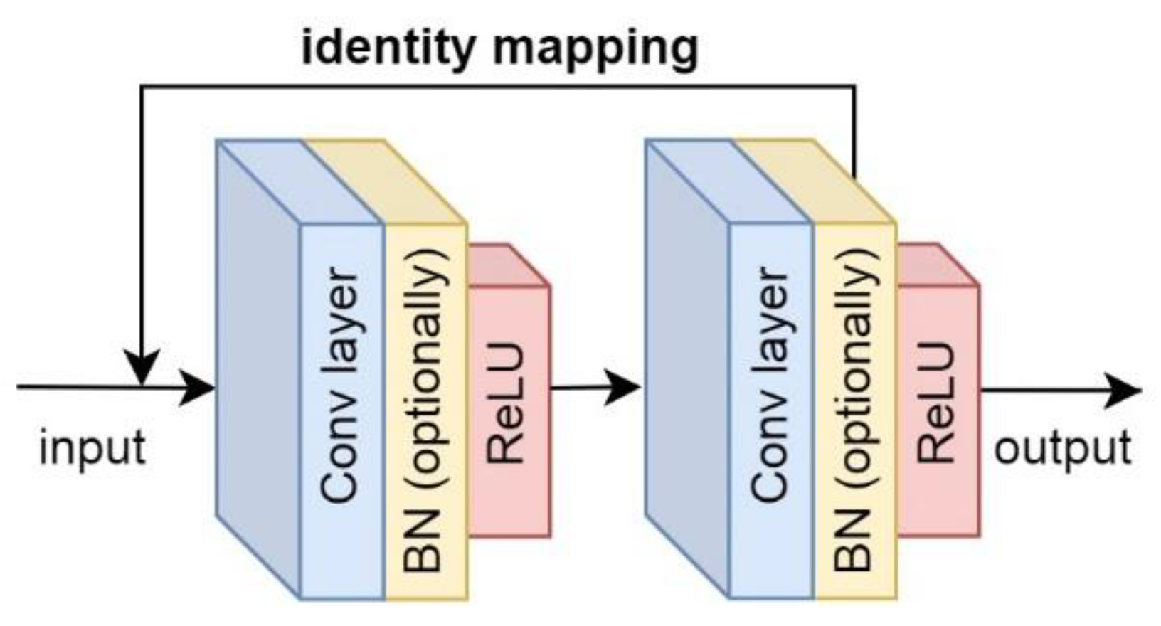
3.3.3. ResNets-Based Solution
In addition to the standard convolutional architecture, we also applied and implemented Residual Networks (ResNets) [
37] to the spectral data classification. It was originally proposed to better cope with the degradation problem in deep CNNs. Details on the architecture are included in
Appendix D.
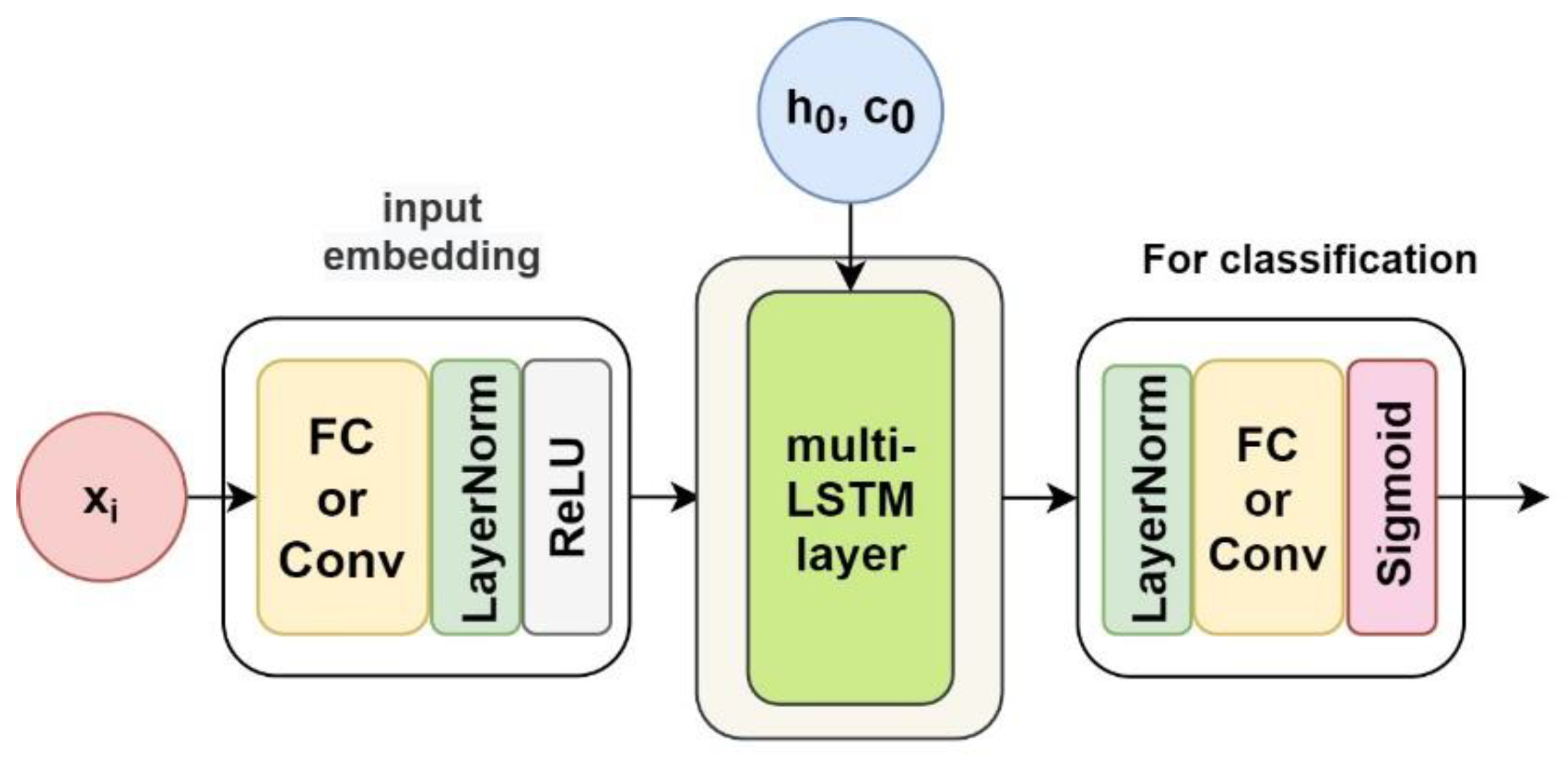
3.3.4. LSTM-Based Solution
As a variance of RNN in particular, Long short-term memory (LSTM) was originally applied in NLP tasks, and it also yielded promising results in time series analysis [
5,
18,
19]. A cell and three gates (input gate, output gate, and forget gate) in the LSTM unit allow this architecture to remember values over arbitrary time intervals and regulate the flow of information [
65]. The pointwise operations used to update the cell state and hidden state in the LSTM architecture can assign different weights to different features/variables in our spectral time series, thereby improving the role of distinguishable features in the classification task and weakening the impact of indistinguishable features on classification. These characteristics make it very suitable for time-resolved spectra analysis. The details of the designed LSTM-based model for spectral data classification are provided in
Appendix E.
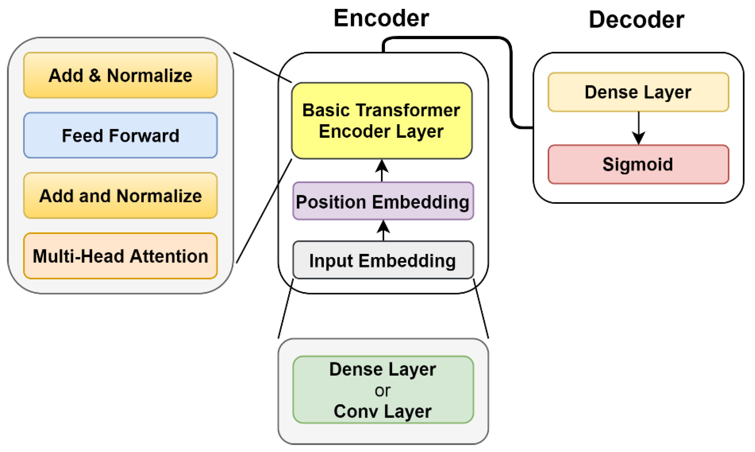
3.3.5. Transformer-Based Solution
The Transformer model relies on the so-called self-attention mechanism and is found to be superior in quality while being more parallelizable [
26]. There are many successful applications of Transformers in time series processing tasks, including classification [
20,
21]. In this work, we adopted the encoder part architecture of the self-attention-based Transformer network as a comparison model, and we show details in
Appendix F.
4. Experiments and Results
In this section, we first introduce the implementation details of the above DL classification models and describe the specific performance metrics we used, and then evaluate and compare their classification performance from multiple perspectives. Further, we conducted a feature importance contribution analysis to explain and interpret these DL classification models. In addition, we analyzed the self-attention scores across the spatial, channel, and temporal dimensions in the convolutional SCT attention model to better investigate its ability to selectively focus on a few classification-related information.
4.1. Implementation Details
All the models are performed in a supervised learning manner and implemented on the Jupyter notebook platform using PyTorch. These models are trained by backpropagation using gradient descent, with the adaptive learning-rate method Adam [
66] as the optimizer (learning rate is set to 8 × 10
−3 for convolutional SCT/SC attention model and 2 × 10
−3 for other models; weight decay is set to 2 × 10
−4 for convolutional SCT/SC attention model and 2 × 10
−5 for other models). We use the binary cross-entropy loss function for our classification task. The statistical models are obtained by minimizing the loss function on the training dataset. All these models are trained on one machine with Tesla P100-PCIE-16GB GPU.
For the end-to-end binned FCNN with the automatically capturing weighting factors model proposed in the 2D space segmentation problem setting, the training dataset consists of 4 original representative spectra samples and 60 simulated ones (by adding some random noise, 15 simulated spectral curves are generated based on each original spectrum), for a total of 64. The reason why we use only a small amount of training data samples in this model is that in this case, the data is only two-dimensional, so the amount of training examples is much larger than the data dimension, which is well-acceptable. The spectra drawn in a dot-dash line and marked in red or blue are used as the basis of the training set, as shown in
Figure 1. In this model, we set the initial training epochs to 550. As the number of bins increases, the training examples in each bin decreases linearly, which may cause the model to easily overfit. To deal with this problem, two early training stop criteria are applied, that is, when the training accuracy is greater than 99.0% or the training loss is less than 0.15. The epochs required during training is shown in
Figure 4.
For the applied models in the 1D time series data analysis setting, there are 31 original spectra samples with 1550 simulated ones as mentioned above (by adding some random noise, 50 simulated spectral curves are generated based on each original spectrum), a total of 1581. The small random noise in the simulated spectral data is generated using the Mersenne Twister [
67] as the core generator. The 31 original spectra samples used as the basis for training are also shown in
Figure 1. Their training information, such as training epochs, training time, memory consumption, etc., are listed in
Table 1. The analysis scripts as Jupyter notebooks are publicly available at
https://github.com/sunyue-xfel/Comparing-End-to-End-Machine-Learning-Methods-for-Spectra-Classification (accessed on 30 November 2021).
4.2. Performance Metric
In this work, our goal is to find the phase transition point, which also means classifying the spectra into 2 phases or classes during the experiment [
12]. As there is no ground-truth phase transition information, we are interested in whether there is a clear classification boundary or an ambiguity zone during the experiment when the classification jumps inconsistently between the phases [
12]. The classification confidence is used as the performance metric, which was defined in our previous work [
12]. It can indicate how small the ambiguous zone is during the experiment. The classification confidence is defined as
, where
represents the number of spectral curves in the classification boundary or ambiguous region with the class label jump,
represents the number of all the tested spectral curves. The classification boundary can be represented by
, where
represents the upper bound or the last spectra of continuous class 0, and
represents the lower bound or the first spectra of continuous class 1. Then
can be calculated by
. Therefore, a clear boundary between these two classes of spectra yields 100% confidence, which would otherwise be less than 100%. Particularly, if no phase transition or boundary between two classes is detected, all the spectral curves are in the ambiguous region, and the classification confidence is 0.
4.3. Quantitative Model Evaluation
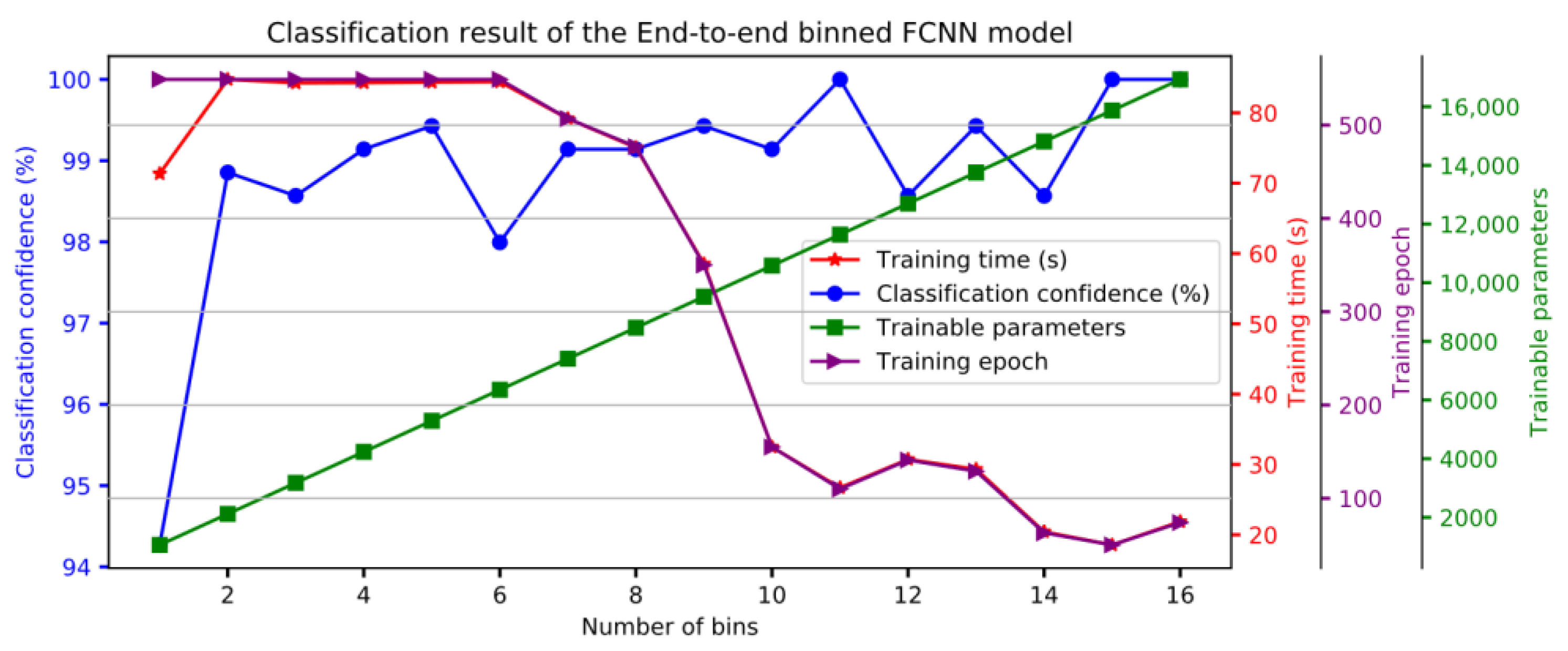
In the 2D space segmentation problem setting, the training information and classification result of the proposed end-to-end binned FCNN with the automatically capturing weighting factors model is shown in
Figure 4. It can be seen from the result that the classification confidence increases as the number of bins increases, and finally achieves 100% confidence. In addition, we can also easily understand that although the trainable parameters increase linearly, as the required training epochs decrease, the required training time also decreases. The classification results show that the binned weighting technique can minimize or even eliminate the impact of misclassification of data points in the overlapping regions with low separability, and even greatly reduce the training time. When using 15 or 16 bins, the model consumes approximately 20 s training time.
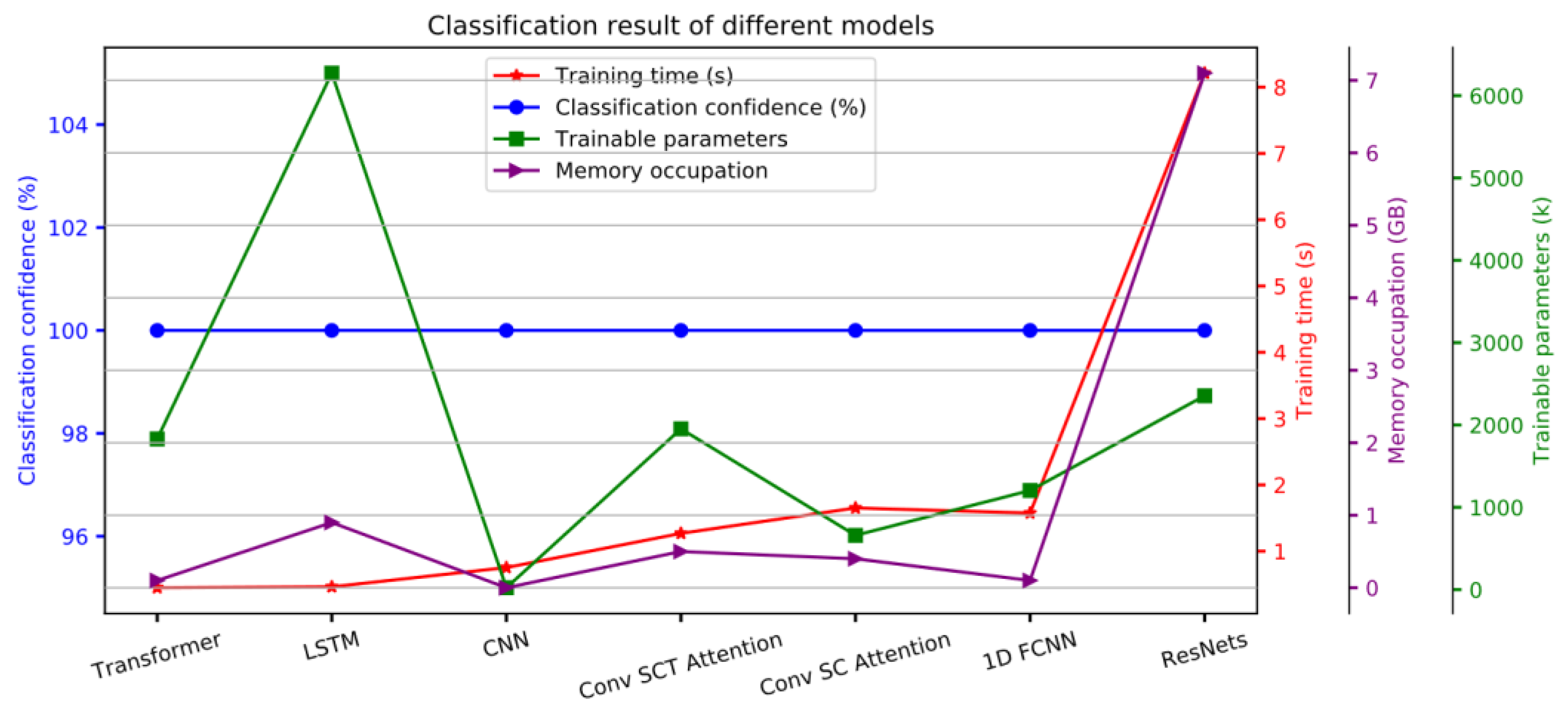
When regarded as a general 1D time series data classification problem, all the applied or proposed models can achieve 100% classification confidence, and the classification boundaries obtained by different models are very stable, and only fluctuate in a small range, that is
, as shown in
Figure 5 and
Table 1. Among these models, the CNN-based model requires the least training parameters. The LSTM-based model has the most trainable parameters, which is mainly introduced by the LSTM units, but its convergence speed is very fast, the training time is short, and the memory consumption is low. Regarding the training time, the Transformer-based model requires the least training time (0.449 s), followed by the LSTM-based model, which needs slightly more training time (0.463 s). At the same time, it can be clearly seen that the curve of memory usage during training has a similar trend to the training time curve. Although the 1D FCNN model requires 300 training epochs, it does not consume so much training time (1.576 s), which is only 3 times that of the LSTM-based model, and it does not consume much memory. From the result, it can be noted that the ResNets model consumes the most time training (8.208 s), and takes up the most memory, but the trainable parameters are still much less than the LSTM-based model. The reason for the long training time may be that there are a bunch of convolution kernels of different scales in this model. The related training information and results are listed in
Table 1.
Nevertheless, the time consumption of ResNets is still much smaller than that of end-to-end binned FCNN with the automatically capturing weighting factors model. In the 2D space segmentation problem setting, the way the model processes data is equivalent to switching from parallel processing to serial processing. The resulting more training examples in 2D space segmentation setting greatly increases the training time. Therefore, although the binned-weighting technique greatly improved the classification performance in the 2D space segmentation problem setting, the models proposed or applied under the 1D time series classification setting are superior.
4.4. Feature Importance Attribution Analysis Based on Gradient Backpropagation
To better interpret the classification models, the feature importance attribution analysis is usually employed to quantify the interpretability of designed networks. An explainable and interpretable classification model would be expected to have an attribution map that can dynamically highlight the highly separable features (corresponding to the peak area in our application) while suppressing the indistinguishable features as much as possible. Since gradients can reflect the influence of each input data point on the current class prediction, and this analysis is model agnostic, does not require ground-truth labels [
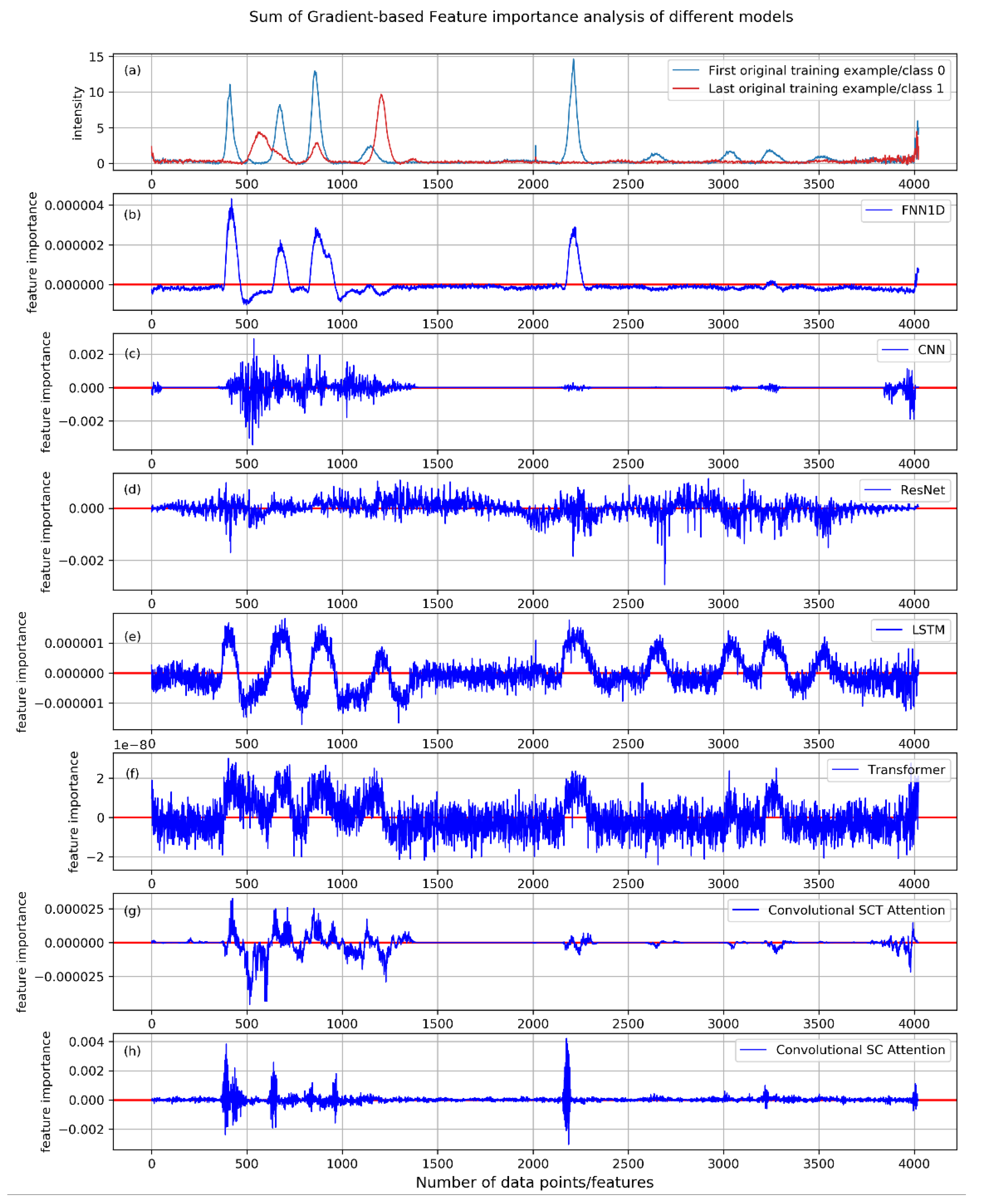
5], we conducted a feature importance analysis based on gradient backpropagation. In this experiment, we estimate the contribution of each input feature on the classification prediction of each model applied under the 1D time series classification setting, as shown in
Figure 6. The contribution map is the cumulative result of all 1581 training examples.
The results of this experiment show that in the 1D FCNN model (
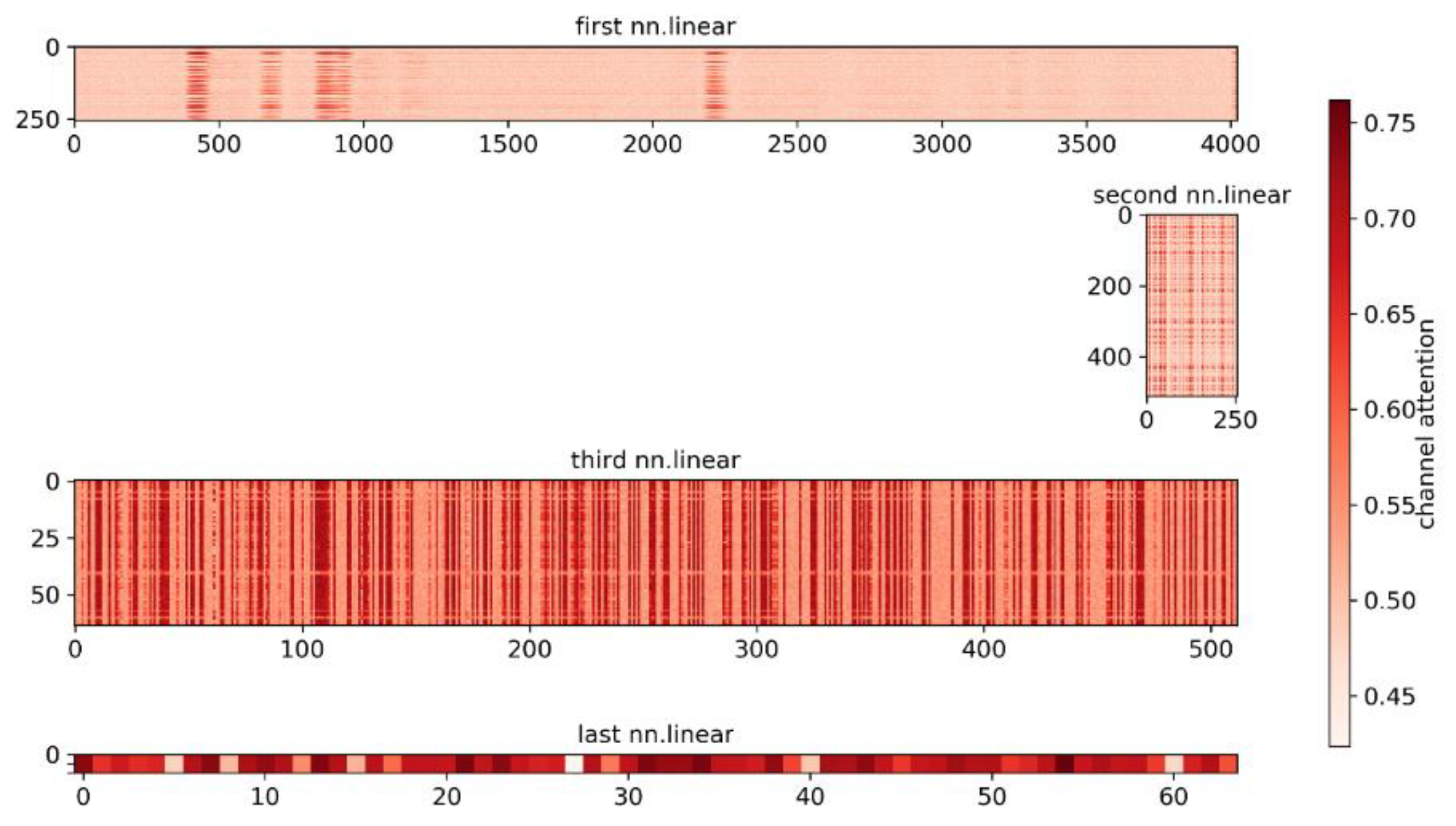
Figure 6b), the feature importance curve maintains a smooth shape, and focuses on most of the obvious features of the spectra. Among them, features close to class 0 obtain a positive contribution value, and features close to class 1 have a negative contribution value. In addition, the contribution of most features in the overlapping area is close to zero, which can reduce the misleading effect of indistinguishable features on classification, and further make the classification-relevant features dominate. Since the 1D FCNN model is only composed of FC layers, it is the most interpretable. The smooth feature importance curve also reflects this point. In order to investigate this further, we visualized the weights learned in each FC layer, as shown in
Figure 7. It can be clearly seen that in each FC layer, only some features are assigned higher weights. The high interpretability of FC layers reveals particularly classification relevant features.
In the CNN-based model (
Figure 6c), the obvious features are also well-highlighted, which further proves the powerful feature extraction ability of the convolution operation. However, one of the imperfections is that the curve is not well-shaped. For ResNets (
Figure 6d), due to the large strides used in the convolution kernel and pooling operations, the feature importance attribution curve of ResNets is more discrete. Its attribution map is also a bit noisy, some indistinguishable features have considerable weight, such as features in the range of 1500 to 2000, but most of the obvious features with high separability are still emphasized.
The gradients through the LSTM-based model (
Figure 6e) and Transformer-based model (
Figure 6f) were a little noisy, its importance values in the overlapping regions are not very well-suppressed We can still easily see that the obtained feature importance contribution curve can well-describe the position and strength of distinguishable features. It can be seen from the importance maps that the features with higher separability achieved higher feature importance values, especially the obvious features with lower intensity values in the latter half of the spectral curve, which are also well-captured.
For convolutional attention networks, most of the obvious features are well-emphasized, and the importance contribution values of the features with low separability is much lower than that of the features with high separability. In the convolutional SCT model (
Figure 6g), the feature importance value of some overlapping regions is even zero, which perfectly suppresses the indistinguishable features with low separability and low classification confidence. In addition, the shape of its feature importance curve is similar to that in the 1D FCNN model, indicating that it has high interpretability. Compared with the convolutional SC attention model (
Figure 6h), it shows its advantages of introducing temporal attention. This indicates that the attention mechanism applied in this model can promote the distinguishable features and suppresses the unobvious and misleading features.
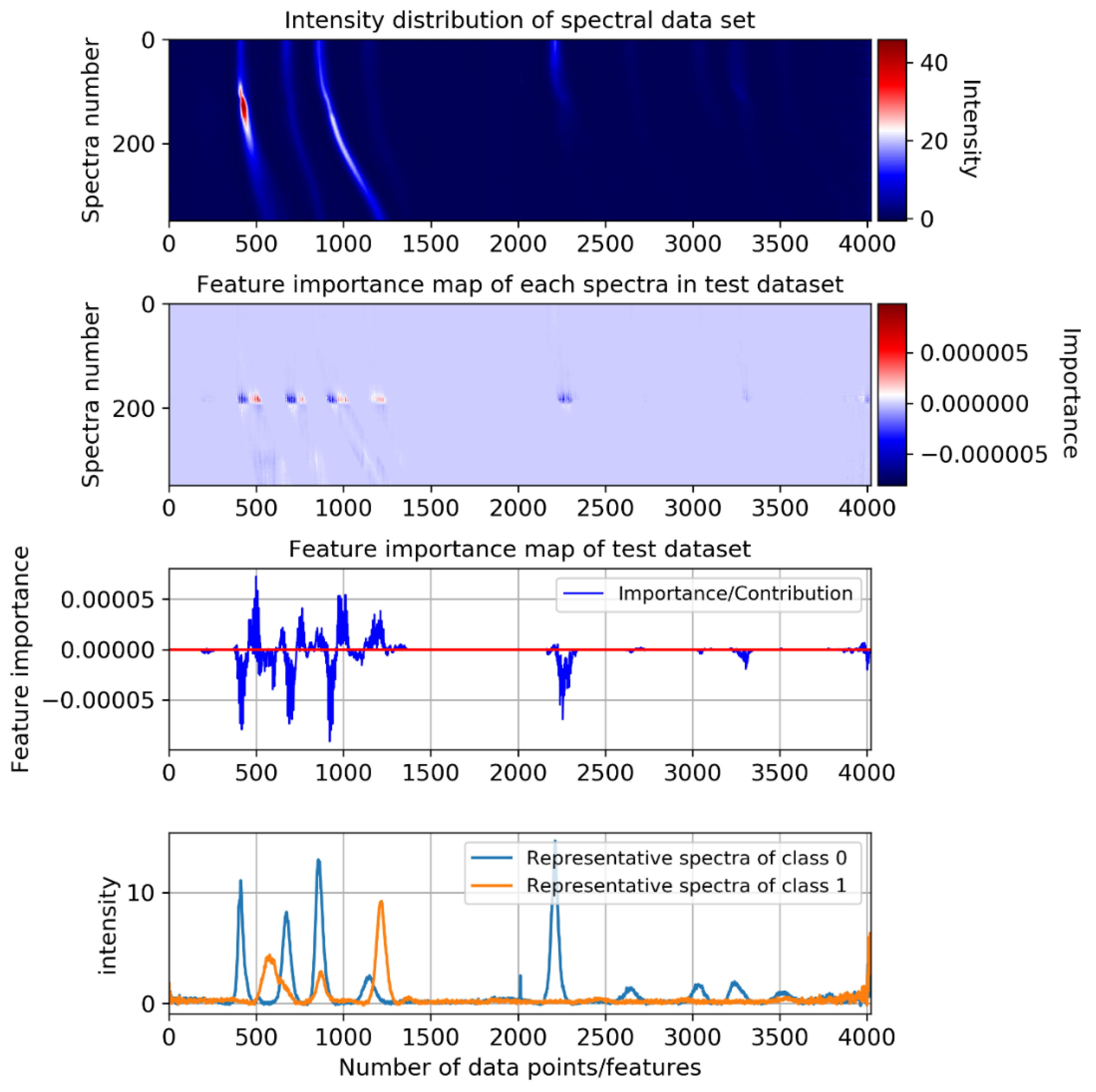
Among all these models, only some of the non-obvious features in the convolutional SCT attention model can reach an importance value of 0, which benefits from the self-attention mechanism applied across three dimensions. We further show its feature importance attribution map of the test dataset in
Appendix G.
The gradient-based feature importance analysis can also be used as one of the references for classification performance, which can be combined with loss function for model training and evaluation. Usually, if the model is not well-trained, the feature contribution map will be rather messy, distinguishing features will not dominate the classification task, and many unobvious features will have a great impact; thereby, reducing the credibility of the classification result.
4.5. Qualitative Analysis of Self-Attention Scores in Convolutional Attention Model
In the feature importance analysis part, we experimentally observed from the contribution map in the convolutional SCT attention models, the distinguishing features can be well-emphasized, which is indicated by high importance contribution values, while the importance values of features in overlapping regions with low separability is close to zero or even zero. It shows the ability to selectively focus on classification-relevant features and suppress the indistinguishable features with low classification confidence. Here, we investigate this further by focusing on the self-attention mechanism performed across spatial, channel, and temporal dimensions and analyze their attention scores.
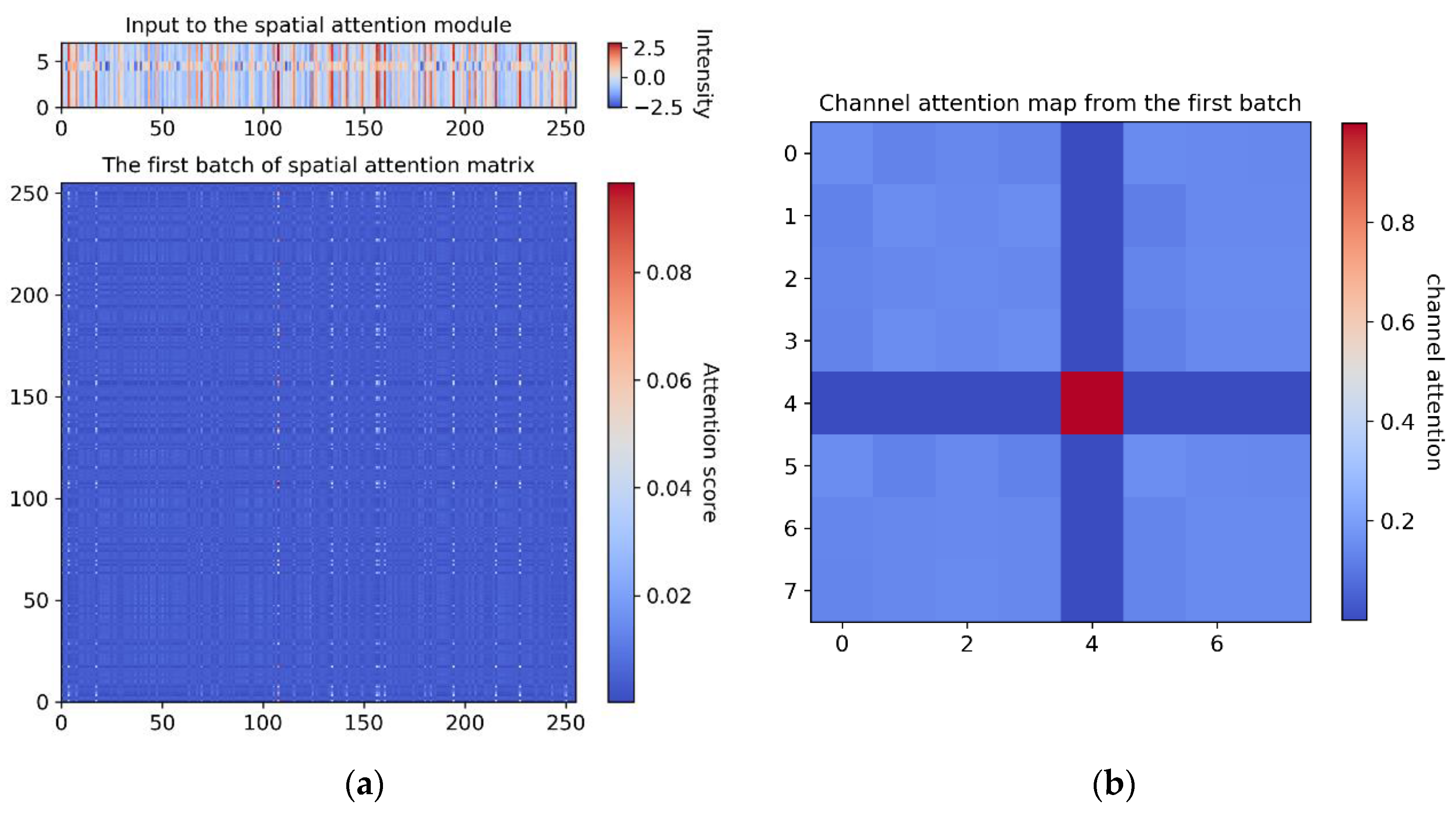
These attention matrixes can be regarded as an adjacency matrix between the input feature vectors and output feature vectors. The attention scores define the dependencies between any two higher-level embedded feature vectors across different dimensions. In our showcase example, the input shape of the spatial attention module and channel attention module is (8, 256). Therefore, the shape of the resulting attention matrix in the spatial dimension and channel dimension are (256, 256) and (8, 8), respectively, as described in
Section 3.2. In this model, the first batch of the input vectors of the spatial attention and channel attention modules are visualized in
Figure 8a, top. The corresponding spatial attention matrix obtained during testing is shown in
Figure 8a, bottom, and the channel attention matrix is visualized in
Figure 8b. From this result, we can understand that only some obvious spatial feature vectors and channel feature vectors are emphasized, which correspond well to the attention matrices. For example, by exploiting the interdependencies between channel maps, we can emphasize interdependent feature maps and further improve feature representation [
64].
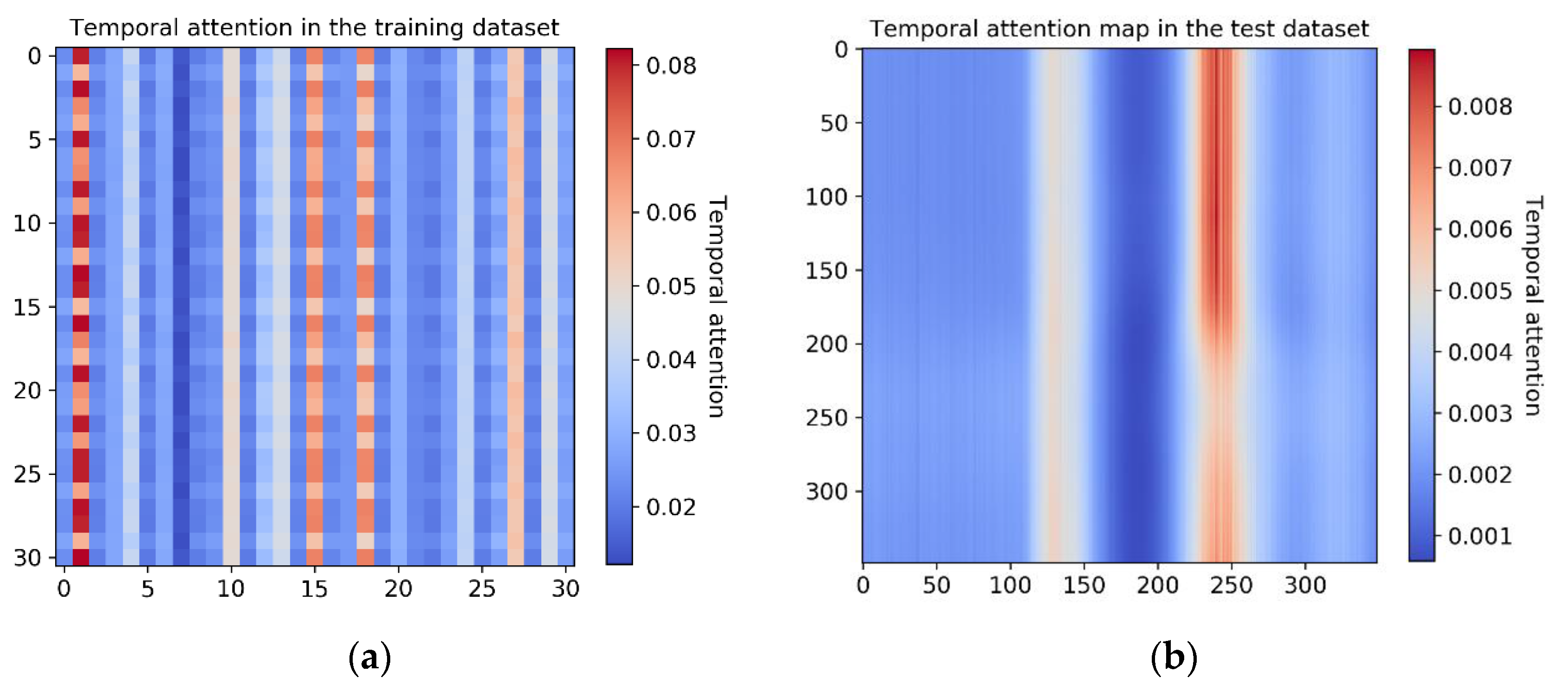
In addition, we also visualized the temporal attention matrices obtained from the training dataset and the testing dataset, and the results show that the self-attention scores only focus on the feature vectors of a few time steps, as shown in
Figure 9. The temporal attention matrix of the test dataset is obtained according to the parameter matrixes learned in the Multi-Head temporal attention module, as described in
Section 3.2.2. From these two temporal attention matrixes, we can find that they have similar shapes, and can selectively focus on some high-level embedded temporal feature vectors that are more relevant to the classification task. In this way, the long-range dependencies modeled across spatial, channel, and temporal dimensions feature greatly enhanced the ability of feature representation.
5. Conclusions and Future Work
In this study, we focus on the application of spectra classification in the fields of diffraction and spectroscopy and on developing and evaluating deep learning classification frameworks for 1D spectral time series. We regard the task either as a 2D space segmentation problem or as a 1D time series data analysis problem. We focus on two proposed classification models, namely the end-to-end binned FCNN with the automatically capturing weighting factors model when viewed as a 2D space segmentation problem and the convolutional SCT attention model when viewed as a 1D time series classification problem. Several other end-to-end model structures based on FCNN, CNN, ResNets, Transformer, and LSTM are explored. Finally, we evaluated and compared the performance of these classification models based on the HED spectra dataset.
In the 2D space segmentation problem setting, for the proposed binned FCNN with the automatically capturing weighting factors model, a quantitative comparison experiment was carried out under different numbers of bins. The classification results show that the classification confidence increases with the increase in the number of bins, while the training time decreases, which means that the binned weighting technique can minimize or even eliminate the effects of misclassifications of indistinguishable features in overlapping regions and speed up the training.
In the 1D time series data analysis problem setting, the 1D FCNN model, CNN-based model, ResNets model, LSTM-based model, Transformer-based model, and our proposed hybrid convolutional attention models are applied, and these models were compared from multiple angles by reporting their classification performance on an HED spectra dataset. Our results show that in this setting, all the models can achieve 100% confidence. Among them, the LSTM-based model and Transformer-based model architecture consume less time (0.463 s and 0.449 s, respectively) compared with the convolutional-based models or the FCNN-based model. Our proposed convolutional SCT attention model also achieved good performance, consuming 1.269 s of training time and does not consume much memory. The CNN-based model has the least trainable parameters and occupies the least memory, while the ResNet model occupies the most training memory and consumes the most training time. As the most time-consuming model, ResNet still uses much less time than the model proposed in the 2D space segmentation problem setting. Therefore, the proposed or applied models under the 1D time series classification setting are superior.
In addition, we investigated all the models in the 1D time series classification setting further through a feature importance analysis using gradients backpropagation. We observed that the 1D FCNN model has the smoothest feature importance map, which also reflects its high interpretability. Further analysis shows that the well-learned weights of each FC layer can focus on most of the obvious features. Moreover, we found that the convolutional SCT attention model has a feature importance map similar to the 1D FCNN model, and the importance value of some indistinguishable features can even reach 0. We studied this further by visualizing the self-attention matrices obtained during training and testing. The results show that the self-attention mechanism performed across spatial, channel, and temporal dimensions can greatly help it focus on obvious features with high separability and suppress indistinguishable feature vectors better than others. These superior characteristics make it suitable for the real-time analysis of experimental spectra data.
It should be noted that our dataset is a very nice representative. All these models implemented in this work can be applied to other spectra datasets generated by other diffraction techniques or spectroscopy techniques, because the spectra have similar characteristics, such as peak increasing, decreasing, broadening, and shifting. We also provide the data analysis scripts as Jupyter notebooks for reproducibility. In addition, the proposed classification models can also be generally applied or easily extended to the classification of any 1D time series.
In this work, only the univariate dataset was tested. In the future, we will improve our DL classification model to make it a general architecture for univariate and multivariate classification tasks. At the same time, multiple datasets from different diffraction or spectroscopy techniques, including univariate and multivariate, will be used for more accurate and reliable evaluation of the algorithms. In addition, the parameters and hyperparameters of these algorithms are currently manually selected. In subsequent research, we will consider conducting parameter analysis work, such as using some optimization algorithms to fine-tune these parameters. We will also further extend our classification model to two-dimensional or three-dimensional image data classification tasks. Finally, learning interpretable, explainable, and generalizable models from data is one of the important directions of our follow-up research.


