A Novel MRE Adaptive Seismic Isolator Using Curvelet Transform Identification

Abstract

Magnetorheological elastomeric (MRE) material is a novel type of material that can adaptively change the rheological property rapidly, continuously, and reversibly when subjected to real-time external magnetic field. These new type of MRE materials can be developed by employing various schemes, for instance by mixing carbon nanotubes or acetone contents during the curing process which produces functionalized multiwall carbon nanotubes (MWCNTs). In order to study the mechanical and magnetic effects of this material, for potential application in seismic isolation, in this paper, different mathematical models of magnetorheological elastomers are analyzed and modified based on the reported studies on traditional magnetorheological elastomer. In this regard, a new feature identification method, via utilizing curvelet analysis, is proposed to make a multi-scale constituent analysis and subsequently a comparison between magnetorheological elastomer nanocomposite and traditional magnetorheological elastomers in a microscopic level. Furthermore, by using this “smart” material as the laminated core structure of an adaptive base isolation system, magnetic circuit analysis is numerically conducted for both complete and incomplete designs. Magnetic distribution of different laminated magnetorheological layers is discussed when the isolator is under compressive preloading and lateral shear loading. For a proof of concept study, a scaled building structure is established with the proposed isolation device. The dynamic performance of this isolated structure is analyzed by using a newly developed reaching law sliding mode control and Radial Basis Function (RBF) adaptive sliding mode control schemes. Transmissibility of the structural system is evaluated to assess its adaptability, controllability and nonlinearity. As the findings in this study show, it is promising that the structure can achieve its optimal and adaptive performance by designing an isolator with this adaptive material whose magnetic and mechanical properties are functionally enhanced as compared with traditional isolation devices. The adaptive control algorithm presented in this research can transiently suppress and protect the structure against non-stationary disturbances in the real time.

1. Introduction

Magnetorheological elastomer (MRE) is a type of composite material whose magnetic field-dependent particles are suspended within non-magnetic elastomer matrix [1,2,3], and is considered a “smart” material. Magnetic field effect can cause variations in stiffness and damping properties and make this material more adaptive and controllable, thereby creating a wide range of prospects for the application of this type of vibration isolation [4,5,6]. The MREs have an ability to change their mechanical properties with the external magnetic field [7,8,9,10,11,12,13,14]. Limited and narrow working frequency bandwidth is regarded as the biggest disadvantage of traditional MR absorbers. To improve the performance of energy dissipation, an MRE-based absorber was studied to enhance shift-frequency property and vibration absorption capacity [15]. An active-damping MRE-based vibration absorber was presented and theoretically analyzed [16]. A frequency tunable passive absorber was developed to suppress vibration and provide good controllability of structures [17]. An axial semi-active MRE-based dynamic vibration absorber was designed to achieve good vibration absorption capacity [18]. The resonance shift property of MRE was studied to verify the nonlinearity and adaptability of the absorber, which had wider effective frequency bandwidths [19]. Due to energy absorption and damping characteristics of MRE absorbers, it is concluded that this material has potential application in seismic isolation [20,21,22,23]. Some scholars have carried out a series of investigations and reviews on MRE Isolators. A proposed variable stiffness and damping isolator was developed by appropriately designing a magnetic circuit optimally passing through MRE layers [24]. An innovative MRE-based isolator was designed with adjustable lateral stiffness to protect structures against near- or far-fault earthquakes [25]. The shear forces were forecasted in real-time and the hysteretic behavior was characterized from the test data of an MRE isolator [26]. An adaptive isolator was developed when a suitable preload and magnetic field were applied together [27]. An MRE isolation system was developed to attenuate the severe vibration of inertial measurement units in three directions [28]. A new variable stiffness and damping isolator was verified in a scaled building with a Lyapunov-based control scheme [29]. The effectiveness of an MRE-based isolation device was proved by implementing it in a single story building structure with fuzzy logic control under seismic excitation [30]. An improved semi-active variable stiffness control law was proposed to achieve better efficiency than traditional on-off control law. The inverse dynamics of an MRE-based isolator was established based on optimal general regression neural network, and an LQR controller was utilized for real-time semi-active vibration control [31]. As a brief review of the literature on the application of MRE materials for seismic isolation indicates, several studies have also been conducted regarding the fabrication and implementation of MRE materials for utilization in civil and mechanical structures. However, to the best of the authors’ knowledge, limited work has been reported on the novel MRE with multiwall carbon nanotubes (MWCNTs), which is a new approach to functionally enhance the magnetorheological behavior of traditional MRE. Compared to traditional MRE, MRE with MWCNTs was developed by mixing carbon nanotubes or acetone contents during the curing process. With such additives, the magnetic-induced property of MRE could be enhanced and improved [32,33]. The MRE with MWCNTs will be a novel MRE adaptive seismic isolator, which is the focus of the study presented in this manuscript.

Micro and macro mechanical properties have always been the focus of scholarly research, which can help us better reveal the physical behavior of materials under stress. The physical phenomenon of MRE is similar to MR fluids. The magnetizable particles are arranged in different ways based on different needs, such as chain and uniform arrangement. The polymer with different particle arrangement is usually regarded as isotropic and anisotropic body. A wide range of applications for this type of MRE has been reported in the literature [34,35,36,37]. A series of investigations and reviews of MRE-type modeling have also been carried out. Mechanical and magnetic properties were simulated and developed by establishing a mechanism of the distribution of magnetic effect [3]. The mechanical response of nanocomposites filled with carbon nanotubes was studied with a viscoelastic interface model [4,5]. A few research studies on theoretical models of MREs were conducted by considering several determinant factors such as magnetic strength, strain amplitude, and loading frequency [6,7,8,9,10,11]. With the excitation of both compressive and shear loading, experimental work was further implemented to modify and validate the conventional magnetorheological model which only took shear effect into account [12,13]. In order to investigate the viscoelastic property of MRE under wider amplitude and variable frequencies, a new revised nonlinear rheological Bouc-Wen model was proposed to consider displacement-, velocity- and acceleration-dependent behavior [14]. These research results show that the mechanical properties of MRE affects the frequency, temperature, magnetic strength, and field dependence modulus. Extensive work on modeling MREs has not been carried out in the literature due to the complexity of this problem. Based on the available MRE models, an MRE with MWCNTs model is studied in this manuscript.

One of the objectives of this paper, is how to assess different constituencies of these materials by using energy distribution. This is a particularly important problem that has not been adequately or methodically addressed, and remains an important research question. A proposed approach to address this problem is to collect microscale images of polymers and analyze them by image recognition methods. The micro-scale image of the edge of mixture is multisingular. In order to solve the shortage of two-dimensional wavelet transform in identifying the Linear Singularity of the edge, a new anisotropic and multiscale curvelet transform is proposed. This approach offers a mapping method which maps a two-dimensional function to a group of two-dimensional directional plane wavelets to obtain curvelet coefficients. Different components of the microstructure of MRE composites need to be clearly differentiated to reveal the weights of each constituen. This is an important task that helps to develop and identify an MRE isolator that is most suitable for seismic application. One of the effective tools that has been employed for feature extraction, in several disciplines, such as structural health monitoring, is wavelet analysis [38,39,40,41,42,43]. Among the wider range of wavelets, the wavelet, proposed by geophysicist J. Morlet in 1981, is an advanced signal processing tool that can adaptively extract features of signals in the time-frequency domain with multiresolution analysis. Due to its unique capability of “zoom lens with an adjustable focus”, it has been widely applied to damage detection and system identification in civil, mechanical and aerospace engineering [44,45,46]. For instance, considering the influence of original defect of structures, wavelet coefficient differences were employed to detect damage locations and quantify specific damages of a beam structure by choosing an optimal scale. As a further development, curvelet performs a better identification efficiency and accuracy in that its anisotropic behavior allows it to “track” the behavior of singularities along curves. This means it can identify an abnormal signal with various scales, spaces and orientations [47]. Curvelet was successfully applied to the identification of non-stochastic surfaces [48], and it was demonstrated that different curvelet scales reflect different energy distribution and features. For the images of MRE in the microscopic level, it is sometimes hard to clearly differentiate mixture types. Therefore, curvelet identification may provide a novel way to explore the features and detailed information of the structure of MRE. Therefore, the curvelet analysis is used to discriminate different material constituents as a new type of “microscope”. To the best of the authors’ knowledge this is the first time that curvelet transform is utilized in this novel application field, i.e., structural health monitoring of composites [49,50].

This study focuses on a comparative study of feature identification of traditional MRE and MREs with MWCNTs, MRE-based isolator design, and the implementation of these “smart” materials in a scaled structure with developed control algorithms. The main focus of this research includes:

(1)

Investigation and modification of parametric models of traditional MRE with functionally enhanced multiwall carbon nanotubes.

(2)

Curvelet identification and feature comparison of MRE and MRE composite structures to MWCNTs using a multiscale Curvelet analysis.

(3)

Adaptive seismic isolator design and magnetic circuit analysis with a novel MRE laminated core structure when the damping system is subjected to both compressive and lateral loading. Development of a reaching law-based sliding mode control and adaptive RBF sliding mode control algorithm for a scaled prototype structure and verification of adaptability, controllability and nonlinearity of the control schemes.

2. Investigation of Five Parametric Models

As the first objective of this theoretical analysis, it is very important to study the physical behavior of MRE materials. MRE is a solid material, and its working mode is mainly shear and tension pressure mode. After the particles are magnetized, they produce a magnetic force. This load causes the matrix rubber to compress. When the particles are stretched or compressed, the interaction force between magnetized particles is related to the displacement between particles. Herein, the constitutive model of the polymer is investigated, which is conducted based on modification of various parametric models of MRE. The following sections present the details of this study.

2.1. MRE Models

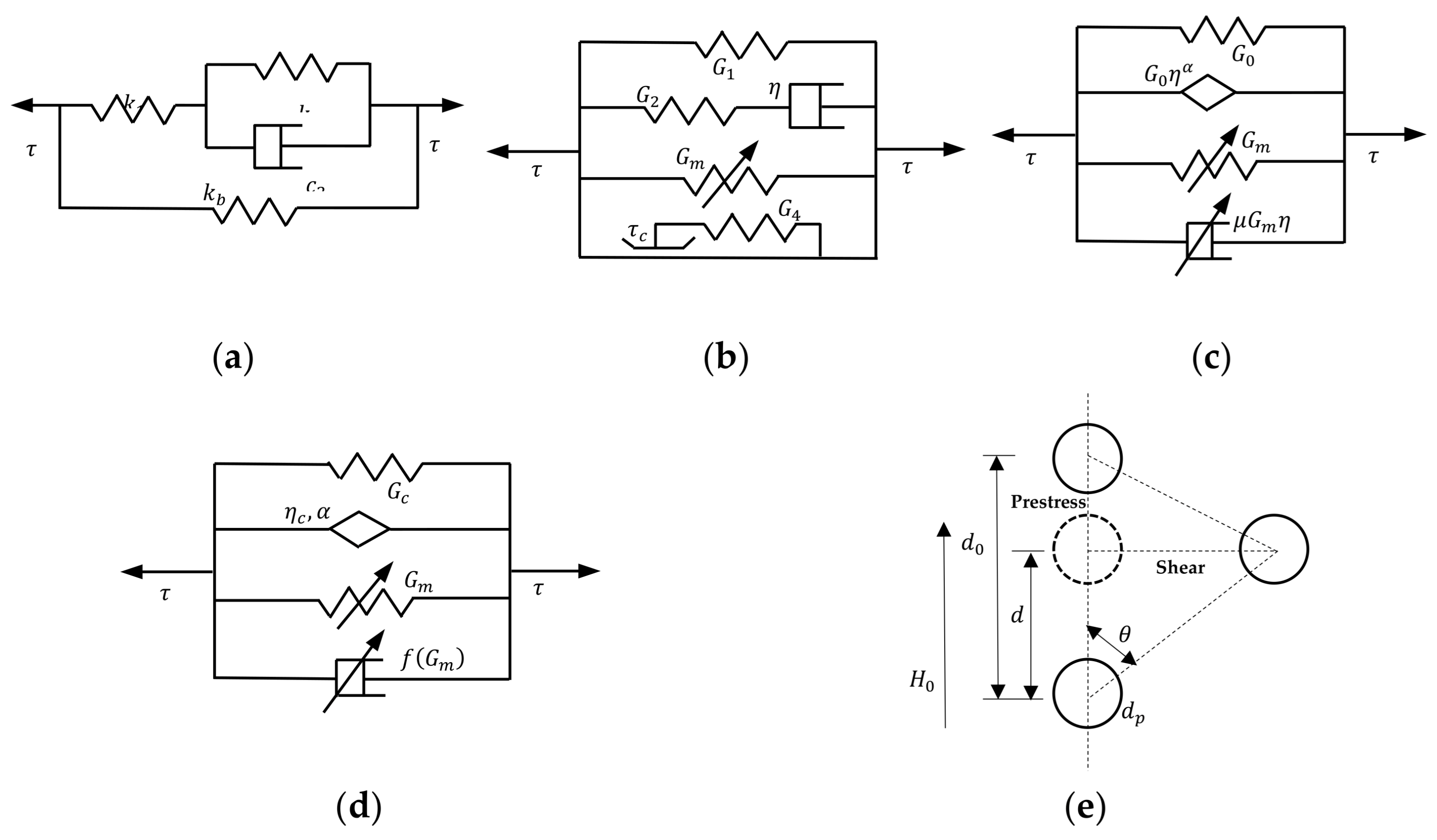
Magnetorheological material is a type of smart material that consists of micron-sized magnetic particles dispersed in an elastomer matrix with specific additives. Its rheological features such as stiffness and damping can change and be controlled reversibly and rapidly by an externally applied magnetic field. If the particles inside the elastomer are uniformly distributed, this material is called isotropic MRE, which is unstructured, while if they have a magnetic-induced, aligned, chain-like columnar structure, it is an anisotropic MRE. In the latter case, a field-dependent aligned particle structure forms and becomes locked in place in the polymer composite during crosslinking processes. To investigate important parametric models derived from Maxwell (a spring and dash-pot in series) and Kelvin (a spring and dash-pot in parallel) models, Laplace transform is employed to present five mathematical expressions of models. Some of the models can be appropriately presented in the time-domain form while others in the frequency domain form. Figure 1 shows these model schematics and the corresponding mathematical expressions are given in

Table 1. Parametric Model of MRE.

No.	Mathematical Expression
M1 [6]	$\tau =\left[\frac{\left(k_1{k}_b+k_2{k}_b+k_1{k}_2\right)\left[{\left(k_1+k_2\right)}^2+c_2^2{\omega }^2\right]+c_2^2{\omega }^2{k}_1^2}{\left(k_1+k_2\right)\left[{\left(k_1+k_2\right)}^2+c_2^2{\omega }^2\right]}+i\frac{c_2\omega k_1^2}{{\left(k_1+k_2\right)}^2+c_2^2{\omega }^2}\right]\gamma$	(1)
M2 [7]	$\tau =G_1\gamma +\frac{\eta G_2\gamma }{\eta +G_{2}t}+\frac{27{\varphi }^2{\mu }_0{\left({\mu }_p-1\right)}^2{M}_s^2{H}^2\gamma \left(4-{\gamma }^2\right)}{4\pi {\mu }_1{\left[M_s+\left({\mu }_p-1\right)H\right]}^2{\left(1+{\gamma }^2\right)}^{7/2}}+\left\{\begin{array}{c}{G}_4\gamma \left|{\tau }_4\right|<{\tau }_c\\ sgn\left(\dot{\gamma }\right){\tau }_c \left|{\tau }_4\right|\ge {\tau }_c\end{array}\right.$	(2)
M3 [8]	$\tau =\left[\left(G_m\left(H\right)+G_0\left(1+{\eta }^{\alpha }{\omega }^{\alpha }\cos \left(\frac{\alpha \pi }{2}\right)\right)\right)+i\left(\mu G_m\left(H\right)\omega \eta +G_0{\eta }^{\alpha }{\omega }^{\alpha }\sin \left(\frac{\alpha \pi }{2}\right)\right)\right]\gamma$	(3)
M4 [9]	$\tau =\left[\left(k_1\frac{G_m+G_c+{\eta }_c{\omega }^{\alpha }\cos \left(\frac{\alpha \pi }{2}\right)}{1+{\left({\epsilon }_0/{\epsilon }_c\right)}^{m_1+m_2}}+b_1\right)+i\left(k_2\left(\omega \mu G_m+{\eta }_c{\omega }^{\alpha }\sin \left(\frac{\alpha \pi }{2}\right)\right)\frac{2{\left({\epsilon }_0/{\epsilon }_c\right)}^{m_1}}{1+{\left({\epsilon }_0/{\epsilon }_c\right)}^{m_1+m_2}}+b_2\right)\right]\gamma$	(4)
M5 [12]	$\tau =\left[G_0+3{\mu }_0{\mu }_m\varphi C{\beta }^2{H}_0^2{\left(\frac{d_p}{d_0}\right)}^3\frac{1}{{\left(1-\epsilon \right)}^3}\left(\frac{4-6{\gamma }^2}{A_1^2{\left(1+{\gamma }^2\right)}^{7/2}}+\frac{12C\beta {\left(d_p/d_0\right)}^3{\left(1-\epsilon \right)}^{-3}{\gamma }^2}{A_1^3{\left(1+{\gamma }^2\right)}^{10/2}}+\frac{5}{B_1^2{\left(1+{\gamma }^2\right)}^{7/2}}+\frac{6C\beta {\left(d_p/d_0\right)}^3{\left(1-\epsilon \right)}^{-3}}{B_1^3{\left(1+{\gamma }^2\right)}^{10/2}}\right)\right]\gamma$ $A_1=4+C\beta {\left(\frac{d_p}{d_0}\right)}^3\frac{1}{{\left(1-\epsilon \right)}^3}\frac{1}{{\left(1+{\gamma }^2\right)}^{3/2}}, B_1=2-C\beta {\left(\frac{d_p}{d_0}\right)}^3\frac{1}{{\left(1-\epsilon \right)}^3}\frac{1}{{\left(1+{\gamma }^2\right)}^{3/2}}$	(5)

Note: In these models, shear strain is the explicit time or frequency-domain function of shear strain or compressive pre-strain. More detailed physical meaning of parameters of these models can be found in the corresponding references.

.

The basic assumptions and applicability of these models include:

(1)

The viscoelastic property is modeled by Maxwell and Kelvin models, and Payne effect is modeled by modified Kraus model.

(2)

The steady state response of shear stress–strain curve is obtained from a harmonic strain excitation $\gamma ={\gamma }_0\sin \left(\omega t+\phi \right)$, where ${\gamma }_0$ is the strain amplitude, $\phi$ is the phase angle, which is the phase angle difference between the input and the output and $\omega$ is the driving frequency.

Model 1 (M1) is a simple linear viscoelastic model. The model is based on the magnetic fluid material three-parameter model. Different from the matrix of magnetic fluid material, the matrix of MRE material is an elastomer, and the effect of matrix deformation is considered. The four-parameter linear viscoelastic model is composed of a three-parameter standard solid model with additional spring element as shown in Figure 1a. In this model, the viscoelastic characteristics of modulus and damping capability is modeled by a three-parameter standard solid model, and the introduced spring element represents field-induced modulus [6]. Model 2 (M2) is a refined model considering the slip between particles and matrix. It consists of three parts: (a) the viscoelasticity of the polymer composite, (b) the magnetic-field-induced mechanical properties, and (c) interfacial slippage between the matrix and the particles. M2 includes a standard linear solid model, a stiffness variable spring, and a spring-Coulomb friction slider as shown in Figure 1b. In this model, the standard three-parameter solid model describes the viscoelasticity of the polymer composite. Magnetic field-dependent property is indicated by various stiffness spring elements by considering the dipole interaction between magnetic particles within the chain, and the interfacial slippage between particles and matrix is modeled by a slider with a threshold of interfacial bond strength [7].

Model 3 (M3) introduces fractional derivative. The stress of time domain is transformed into a complex modulus (storage modulus and dissipation modulus) by Fourier transform. This is different from the traditional Newton pot (Figure 1a,b), which can only express the behavior of viscosity. The fractional order introduces frequency into the storage modulus, so the viscoelastic behavior becomes the spring pot in Figure 1c. The spring pot can express the behavior between elasticity (called storage modulus) and viscosity (called dissipation modulus), which is more consistent with the actual physical experimental behavior. M3 is a parametric magneto–viscoelastic model that includes four parallel elements, i.e., a spring element, a fractional derivative dashpot element, a nonlinear spring element and an additional analogous dashpot element, as shown in Figure 1c. In this model, the spring element together with the fractional derivative dashpot element represent the viscoelasticity of the matrix. Magnet field-dependent phenomenon is indicated by a nonlinear spring, and the damping variance with induced magnetic field is represented by the analogous dashpot element [8].

Model 4 (M4) is a model describing the experimental physical phenomenon that the polymer strain falls when it reaches a certain value. This physical phenomenon is called the Payne effect. When strain increases, the structural mesh is destroyed rapidly, and the elastic model decreases rapidly. M4 is an extended fractional derivative model with further modification of M3, as shown in Figure 1d. In this macroscopic model, the spring element represents static and elastic shear modulus. Viscosity coefficient along with fractional order element are considered determinant factors of viscosity of composite. The variable and nonlinear stiffness and damping elements describe magnetic-induced behavior. In addition, Payne effect is taken into consideration with a modified Kraus model that describes the influence of Van Der Waals interactions and friction between particles and matrix on breaking and rebuilding processes [9]. M2 is a mathematical model in the time domain. M1, M3 and M4 are mathematical models represented with Laplace transform, where the real and imaginary parts of the expression respectively represent the storage modulus and loss modulus of the complex modulus.

Model 5 (M5) considers the pre-strain under the action of magnetic field. Starting from the chain structure of particles in the matrix, the dipole theory of the linear chain is used for modeling. The magnetic field direction is vertically upward, and the center distance of the dipole (magnetized particles) arranged along the magnetic field direction is d0, as shown in Figure 1e. When the dipole is deformed to the dotted circle position of Figure 1e, the two dipoles will generate energy. The conversion of magnetic field energy and matrix strain energy results in magnetic-induced modulus (including magnetic-induced Young’s modulus and magnetic-induced shear modulus). Its size is related to particle spacing, particle volume ratio and saturation strength of magnetic field. So M5 is a microscopic model that simultaneously includes the effects of magnetic energy density, shear strain and pre-strain [12]. The parameters in these models have been identified and verified using an objective function based on the data from analytical and experimental work.

2.2. Model Attribute

From

Table 2. Model Attribute.

No.	Viscoelasticity	Magnetic Field	Strain Amplitude	Loading Frequency	Payne Effect	Shear Strain	Compressive Prestrain	Macroscopic Model	Microscopic Model
1	◯	◯	◯	◯	✕	◯	✕	◯	✕
2	◯	◯	◯	◯	✕	◯	✕	◯	✕
3	◯	◯	◯	◯	✕	◯	✕	◯	✕
4	◯	◯	◯	◯	◯	◯	✕	◯	✕
5	✕	◯	✕	✕	◯	◯	◯	✕	◯

Note: ◯ denotes the model has this type of attribute, while ✕ represents the model does not have this type of attribute.

, a comparative study on different kinds of model attributes is further discussed based on the research conducted by previous scholars [6,7,8,9,10,11,12,13]. M1-M4 are macroscopic models denoting the viscoelastic properties of MRE. These models can show the relationship between shear stress and shear strain, and are functions of magnetic field, strain amplitude and loading frequency. However, none of them can consider the effect of pre-strain, and only M4 can incorporate the Payne effect due to the consideration of the element of modified Kraus model.

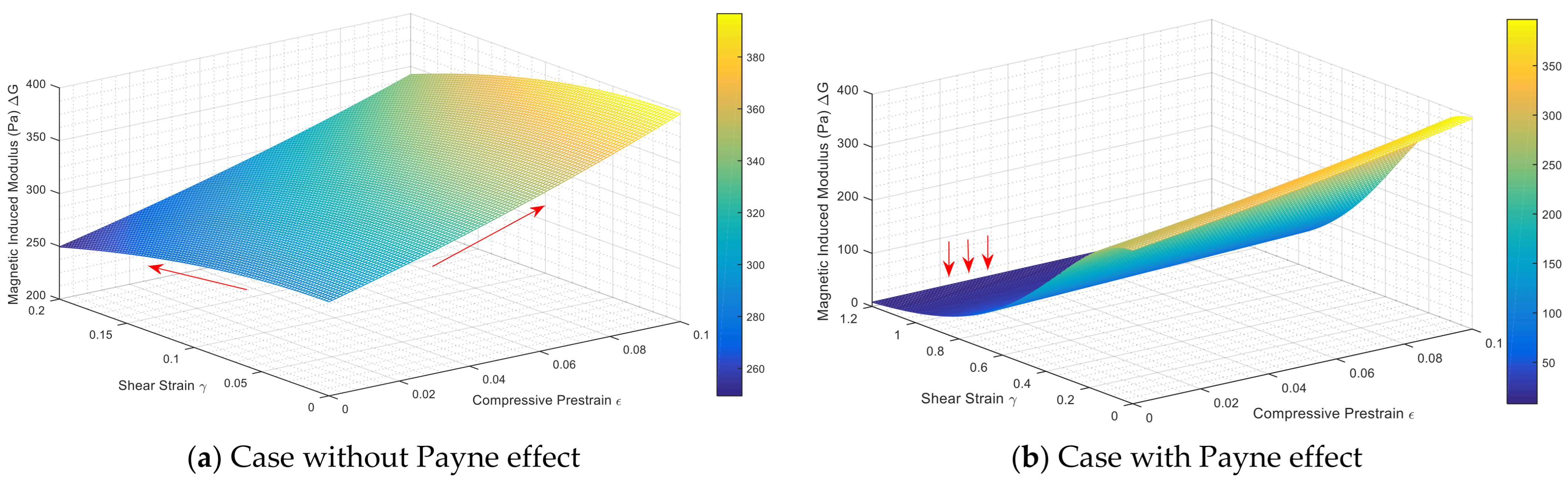
Specifically, as shown in Figure 2a, M5 reveals the relationship between magnetic-induced modulus $∆G$ versus lateral shear strain $\gamma$ and compressive pre-strain $\epsilon$. It is obviously found that $∆G$ is positive with the shear strain $\gamma$ increasing, while the gradually increasing compressive prestrain $\epsilon$ has a positive effect on the magnetic-dependent modulus. However, if the lateral shear effect is considerably large, such as seismic effect with large acceleration and random vibration, the dynamic strain will cause decreasing dynamic stiffness and growing energy dissipation. In this case, the elastomer has a large deformation and the breakdown of filler networks initiates. At the same time, the interaction of particles attenuates as the distances of particles within and between chains increase, which gives rise to a decreasing trend of both storage modulus and loss modulus.

This phenomenon is more visually indicated in Figure 2b. The magnetic-induced modulus $∆G$ becomes zero and even negative in the large shear-deformation area ($\gamma$ = 1.2 in the extreme case). Therefore, M5 is more suitable for comprehensively considering both Payne effect of shear loading and pre-stress in the micro scale when MRE is simultaneously subjected to external magnetic excitation, lateral shear and vertical compression.

2.3. MRE with MWCNTs Models

Carbon nanotubes are small sized materials that have low density and high aspect ratio. The bonding between elastomers and magnetic particles can be generally improved with reinforcing MWCNTs, thus the corresponding MR effect is higher. Experimental study was conducted to modify the previously discussed parametric models. With the dispersed MWCNTs in the liquid elastomer with sonication, which was later mixed with magnetic particles, the curing process could be completed under a steady magnetic field. Carbonyl iron powders with average diameter of 8 μm were used as magnetic particles, and silicone rubber was as elastomer. Iron particles are chosen in MRE because of their high permeability, low remnant and saturated magnetization ability. MWCNTs with a diameter of 10 nm and length ranging from 10–15 μm and 95 wt% purity were used as additives. About 30 wt% of iron particles and 1.5 wt % of MWCNTs were mixed in the solution and fabricated in the matrix. The mixture molds were placed between permanent NdFeB bar magnets to form stable polarized structured particle chains under the field strength of 1.35 T.

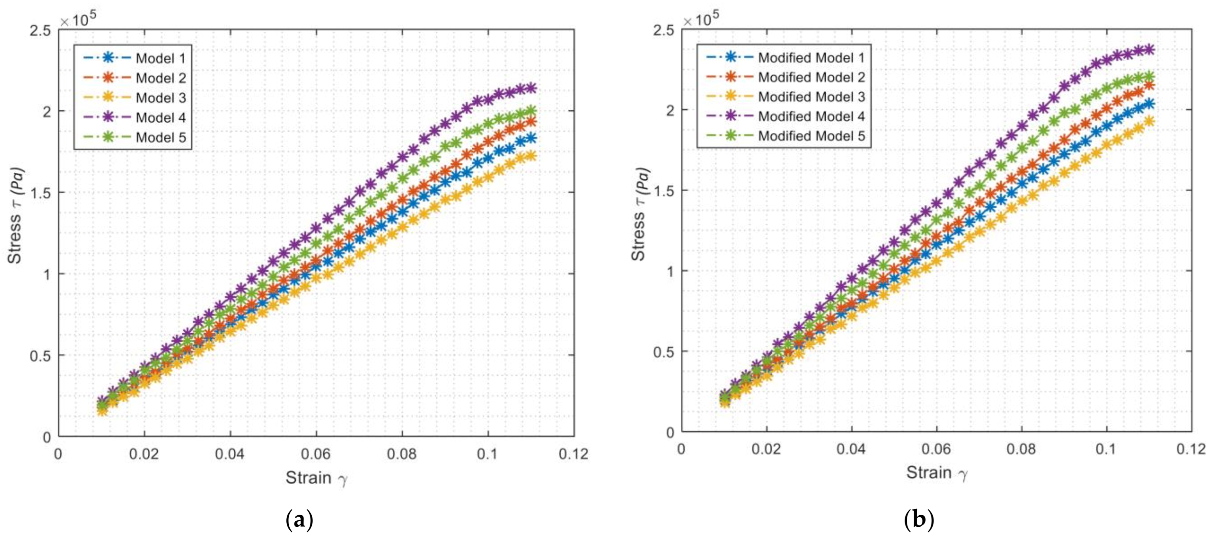
For M1 to M4, a parallel spring element ($\tau =G_{MWCNT}\gamma$) is added to modify the aforementioned MRE models by considering the effect of MWCNTs, which functionally enhance the traditional magnetorheological elastomer. Model 5 can be improved by modifying relative permeability of matrix μm. As shown in Figure 3, the shear stress-strain curves for magnetorheological elastomer nanocomposites are measured at the magnetic field 1 T, strain amplitude 11% and loading frequency 1 Hz. In Figure 3, for MRE, the elastic part of the curve represents initial modulus, i.e., 1.74 MPa, 1.81 MPa, 1.62 MPa, 2.13 MPa and 1.96 MPa for M1-5, respectively. Compared with initial stiffness at the strain amplitude of 0.11, the modulus for M4 and M5 are 1.95 MPa and 1.81 MPa, which show, respectively, 8.45% and 7.65% loss of initial modulus. For MRE with MWCNTs, the values of modulus for the elastic parts are 1.94 MPa, 2.03 MPa, 1.77 MPa, 2.38 MPa, 2.17 Mpa, respectively, for modified M1-M5. Compared with initial stiffness at the strain amplitude of 0.11, the modulus for M4 and M5 are 2.15 MPa and 2.01 MPa, which show, respectively, 9.66% and 7.37% loss of initial modulus.

These models are modified due to the fact that stronger interaction between fillers and matrix has larger positive effect on the storage modulus, and the loss factor or damping is more influenced by the friction between particles and matrix molecular chains that leads to more degrees of molecular mobility and energy dissipation. Payne effect can be obviously observed in macroscopic M4 and microscopic M5. Large magnetic field effect and strain effect will increase the energy of magnetic particles, which move away from each other and thus, reduce the interaction and cause breakage of physical bonding. In general, with strain amplitude increasing, both storage modulus and loss factor show a descending trend. This phenomenon is in accordance with the Payne effect.

When the applied magnetic field increases, MRE and MR nanocomposites perform better storage modulus and loss factor, which indicates stronger MR effect. MR nanocomposites generally show higher MR effect than conventional MRE under the same condition. With applied current increasing, the increased magnetic field will form stronger magnetic flux density which results in enhanced storage modulus with related to stiffness and loss modulus related to damping property. Moreover, storage modulus decreases with increased magnetic intensity. On the contrary, loss modulus has consistent trend of change in regard to magnetic intensity. These magneto-viscoelastic properties and related models have been tested and verified and will be later applied to modeling viscoelastic behavior of MRE material as a core structure of the isolator [12,32,33,51].

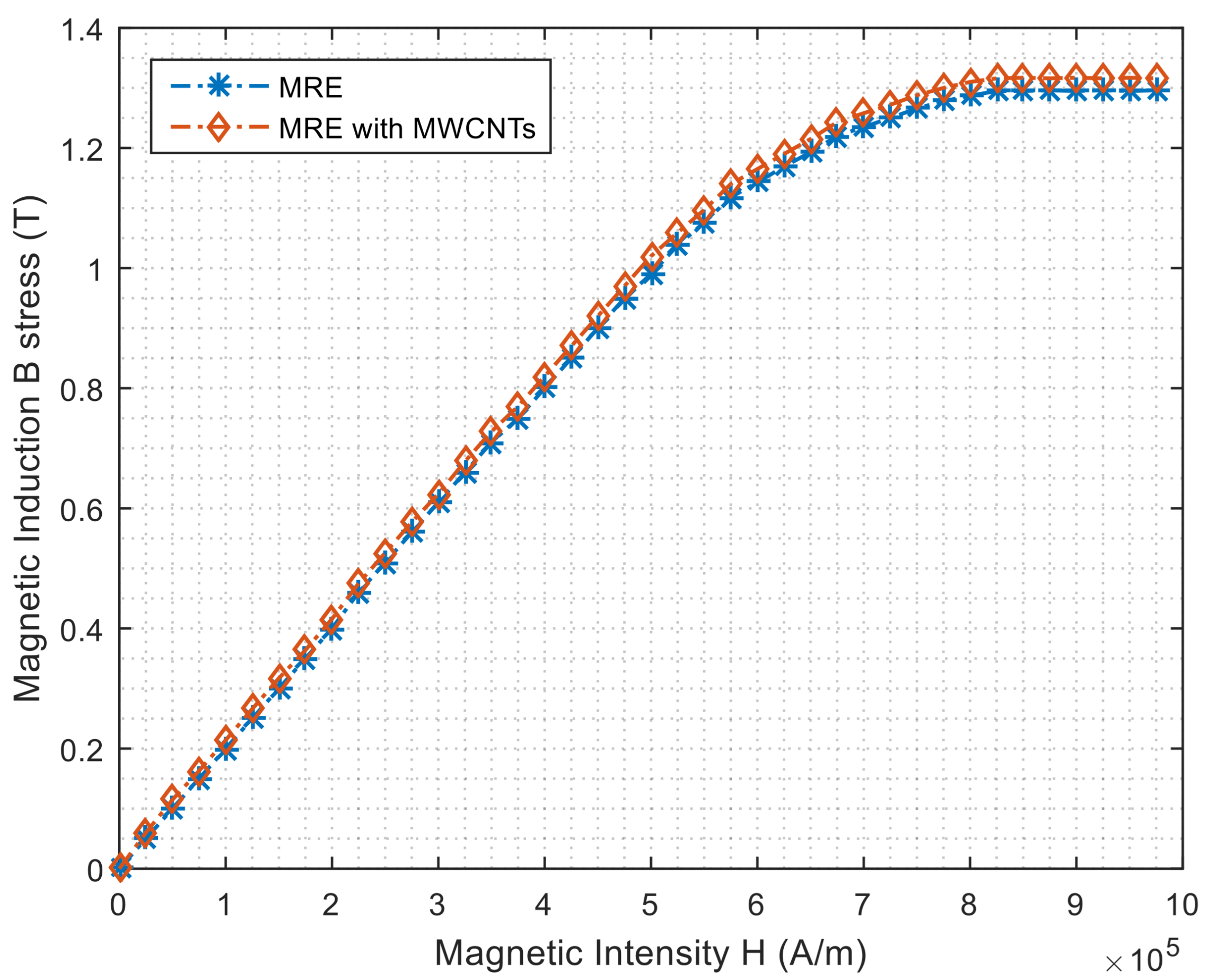
Other experimental work was to test the change of magnetization effect when the traditional MRE is enhanced by multiwall carbon nanotubes. In the experiment, vibrating sample magnetometer was used to acquire magnetization curves of MRE and MRE nanocomposite. The externally applied magnetic field varied between 0–1.5 T. Hysteretic curve for MRE and MRE nanocomposite samples were measured as shown in Figure 4. The saturation magnetization curve shows the relationship between magnetic strength $H$ and magnetic induction $B$ for MRE and MR nanocomposite during the magnetization process. It can be denoted that the saturated magnetic induction for MRE and MRE with MWCNTs is 1.296 T and 1.316 T, respectively.

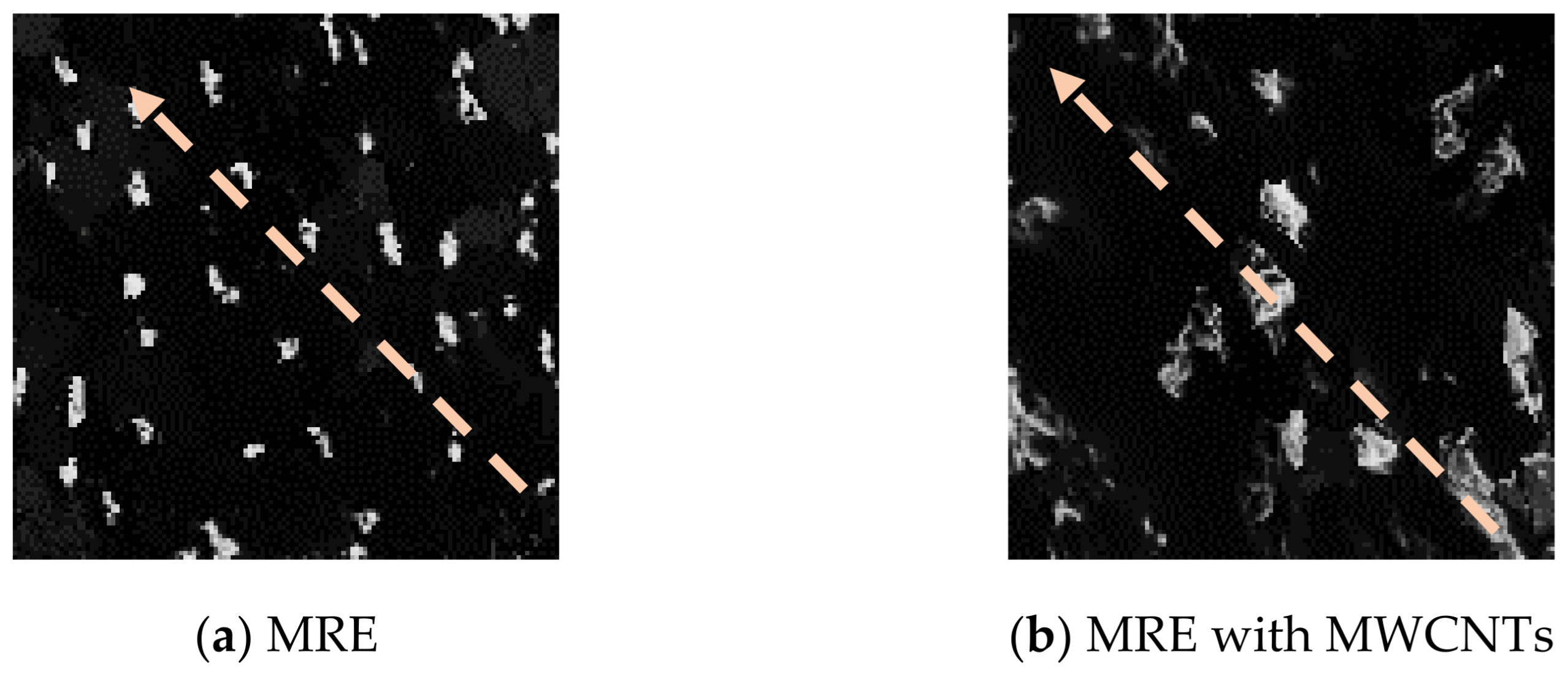
Figure 5 illustrates the samples of traditional MRE and MRE filled with MWCNTs with a scanning electron microscope (SEM). The dashed arrow denotes the direction of applied magnetic field when particles in the matrix are energized. As can be seen, with the addition of MWCNTs, nanocomposites wrap up iron particles, forming a more stable bonding property between the matrix and the particles.

3. Curvelet Identification of MRE and MRE with MWCNTs

In this section, curvelet transform is introduced as a novel image characteristic identification tool to reveal different constituents of both fabricated conventional MRE and MRE with multiwall carbon nanotubes.

3.1. Curvelet Transform

Curvelet transform is a mapping principle expressed as a transform $f\to {\Gamma }_f\left(a,b,\theta \right)$ of a function $f\left(x_1,x_2\right)$ on $R^2$ into a transform domain regarding a specific scale $a>0$, location $b\in R^2$, and orientation $\theta \in \left[0,2\pi \right)$. The function assumed herein is on the two-dimension plane $R^2$ with spatial variable $x$, frequency-domain variable $\xi$ denoted with $r$ and $\omega$ polar coordinates. Radial and angular windows are respectively expressed as $W\left(r\right)$ and $V\left(r\right)$. They satisfy admissibility conditions:

$${{\displaystyle \int }}_0^{\infty }W{\left(ar\right)}^2\frac{da}{a}=1, \forall r>0$$

(6)

$${{\displaystyle \int }}_{-1}^{1}V{\left(u\right)}^{2}du=1$$

(7)

A family of analyzing elements can be constructed using these windows. At scale $a$, the family is generated on the basic element ${\gamma }_{a00}$ with different levels of transition and rotation.

$${\gamma }_{ab\theta }\left(x\right)={\gamma }_{a00}\left(R_{\theta }\left(x-b\right)\right)$$

(8)

Accordingly, the Polar Fourier coordinates $\left(r,\omega \right)$ at the scale $a$ are defined as:

$${\widehat{\gamma }}_{a00}\left(r,\omega \right)=W\left(ar\right)V\left(\omega /\sqrt{a}\right)a^{3/4}$$

(9)

Thereby, the support of ${\gamma }_{ab\theta }$ can be expressed as combination of polar “wedge” shapes with scale-dependent radial and angular windows in different directions.

Continuous curvelet transform ${\Gamma }_f$ can be defined with different scales, locations and directions in space.

$${\Gamma }_f\left(a,b,\theta \right)={\gamma }_{ab\theta },f a<a_0,b\in R^2,\theta \in \left[0,2\pi \right)$$

(10)

Assuming $V$ and $W$ satisfy admissibility conditions, the $Calder\acute{o}n$-like reproducing formula for high-frequency functions is expressed as:

$$f\left(x\right)=\int {\Gamma }_f\left(a,b,\theta \right){\gamma }_{ab\theta }\mu \left(dadbd\theta \right)$$

(11)

where a Parseval formula for high-frequency functions is:

$${\Vert f\Vert }_{L^2}^2=\int {\left|{\Gamma }_f\left(a,b,\theta \right)\right|}^2\mu \left(dadbd\theta \right)$$

(12)

Assuming $\mathsf{\Phi }$ is a band-limited radial function in $L^2$

$${\mathsf{\Phi }}_{a_0,b}\left(x\right)=\mathsf{\Phi }\left(x-b\right), \mathrm{thus}$$

(13)

$$f\left(x\right)=\int ⟨{\mathsf{\Phi }}_{a_0,b},f\rangle {\mathsf{\Phi }}_{a_0,b}\left(x\right)db+{{\displaystyle \int }}_0^{a_0}\iint ⟨f,{\gamma }_{ab\theta }\rangle {\gamma }_{ab\theta }\mu \left(dadbd\theta \right) , \mathrm{and}$$

(14)

$${\Vert f\Vert }_{L^2}^2=\int ⟨{\mathsf{\Phi }}_{a_0,b},f^2\rangle db+{{\displaystyle \int }}_0^{a_0}\iint ⟨f,{\gamma }_{ab\theta }\rangle {}^2\mu \left(dadbd\theta \right)$$

(15)

Therefore, the “full” curvelet transform consists of the fine-scale directional elements and coarse-scale isotropic father wavelets.

Conventional Fourier transform can map a function to a combination of a series of trigonometric bases with limited frequency domain information. Wavelet transform can identify horizontal, vertical and diagonal details with poor directional selection ability but may lose the feature of edges with changing orientations and angles. Thus, it cannot effectively deal with line singularity. The biggest advantage of curvelet transform is that it can extract spatial and directional feature information with optional-scale multiresolution analysis. Curvelet has a good property of representing border lines with highly directional anisotropy and sensitivity regarding various locations, orientations and scales of curved morphological structures at the same time, rather than just simple thresholding.

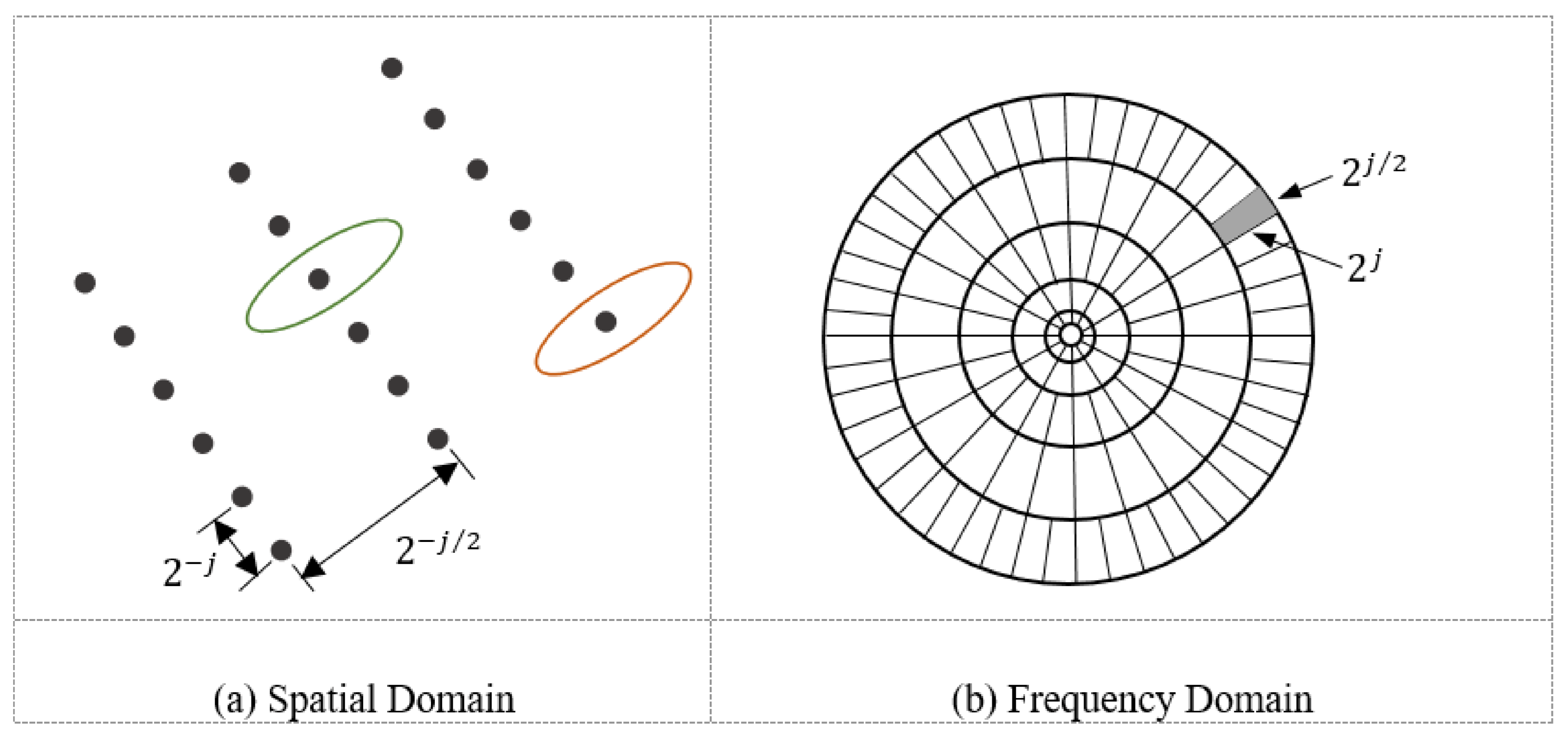
As shown in Figure 6, the spatial Cartesian grid is related to a specific scale and orientation, while in the Fourier space, curvelet is supported near a “parabolic” wedge indicated with a shaded area in the frequency plane.

3.2. Curvelet Identification

Due to various and complex morphological patterns of features of images, sparse representation in the curvelet domain is required so that one type of feature can be identified via one or several related decomposed terms. The maximum number of decomposed scales is ${\log }_{2}N-3$ for an $N\times N$ image. Three steps are implemented for feature extraction. First, an image is decomposed via curvelet transform into multiple scales with different orientations and angles. Second, different regular main features of decomposed components in the transform domain are grouped and clustered at large scales while irregular and isolated dots or noise denoting other features are obtained and classified into other groups. Finally, inverse curvelet transform is applied for reconstruction of features based on different scales. The SEM image of MRE and nanocomposite has the size of 128 pixel $\times$ 128 pixel. The maximum number of decomposition scale via curvelet is ${\log }_{2}128$ − 3 = 4. 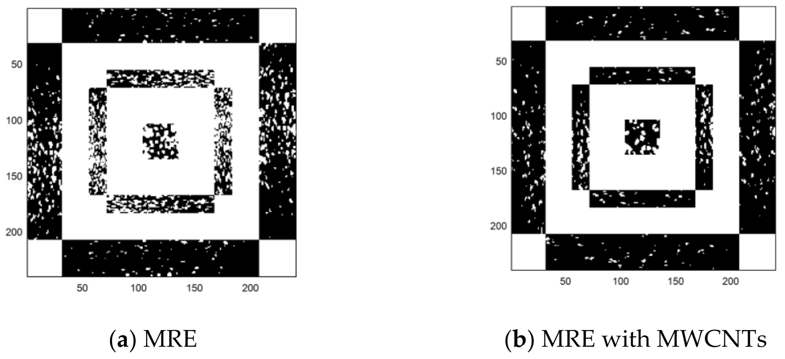Figure 7 shows the absolute values of coefficients of curvelet transform, where coefficients in different scales are distinguished by interval gray bands indicating no curvelet coefficients. Areas in lighter color represent larger value of coefficients, which means more energy is distributed.

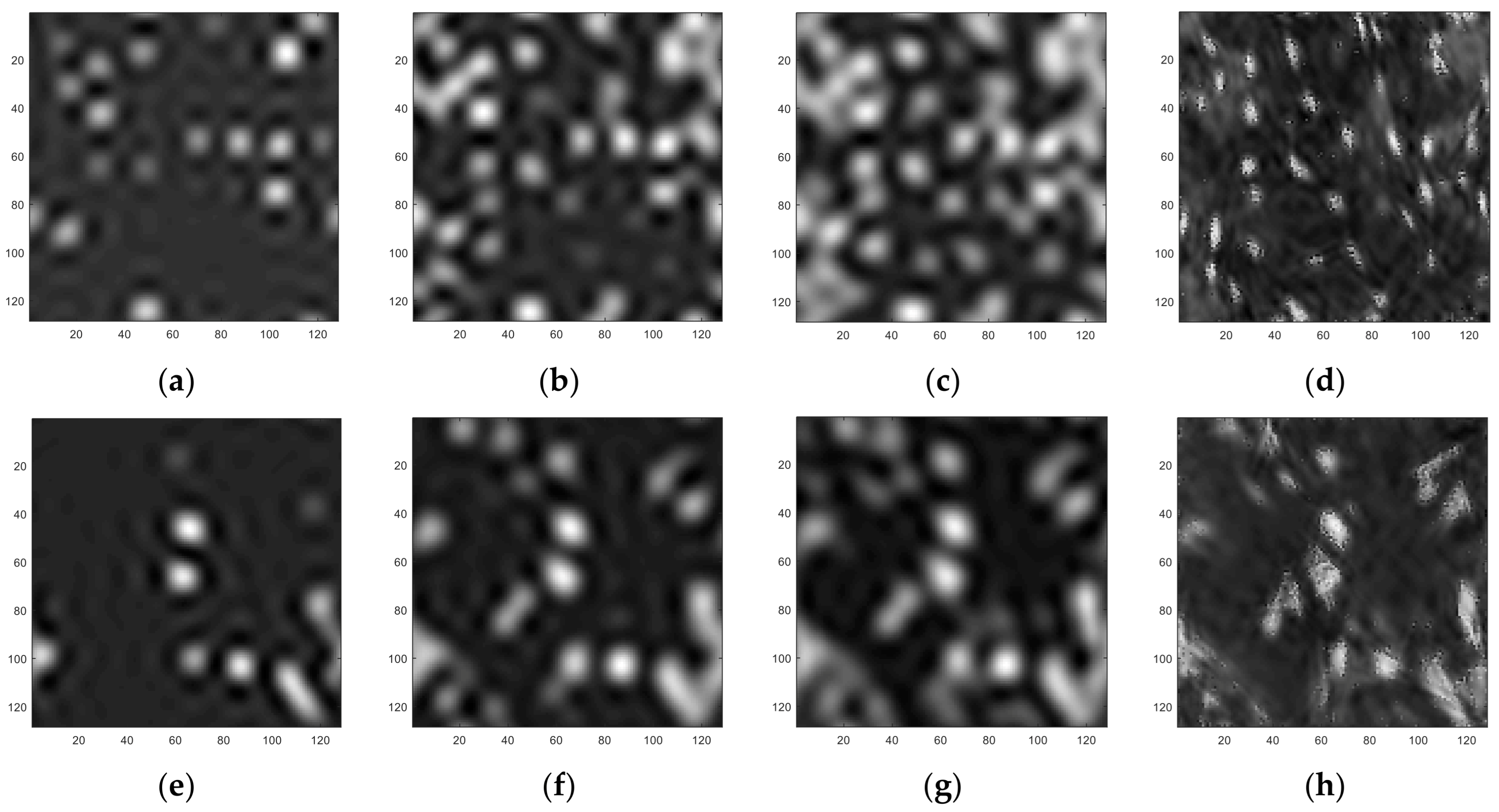
Illustration of reconstructed image at each scale is shown in Figure 8. For both MRE, and MRE with MWCNTs, the first scale reveals the coarse and overall characteristics of the composites, the second and third scale reflects more concrete composition of the composites in the curvelet domain, and the forth scale shows the finest part and a few noise effects on the image.

Areas in strip-shape light color are denoted as iron particles, dark colors are silicon rubber matrix, and cotton-like material with small clusters is the additives of MWCNTs. Specifically, scale four of MR nanocomposite reveals MWCNTs closely wrap the scattered iron particles, showing a distinct bonding between matrix and particles.

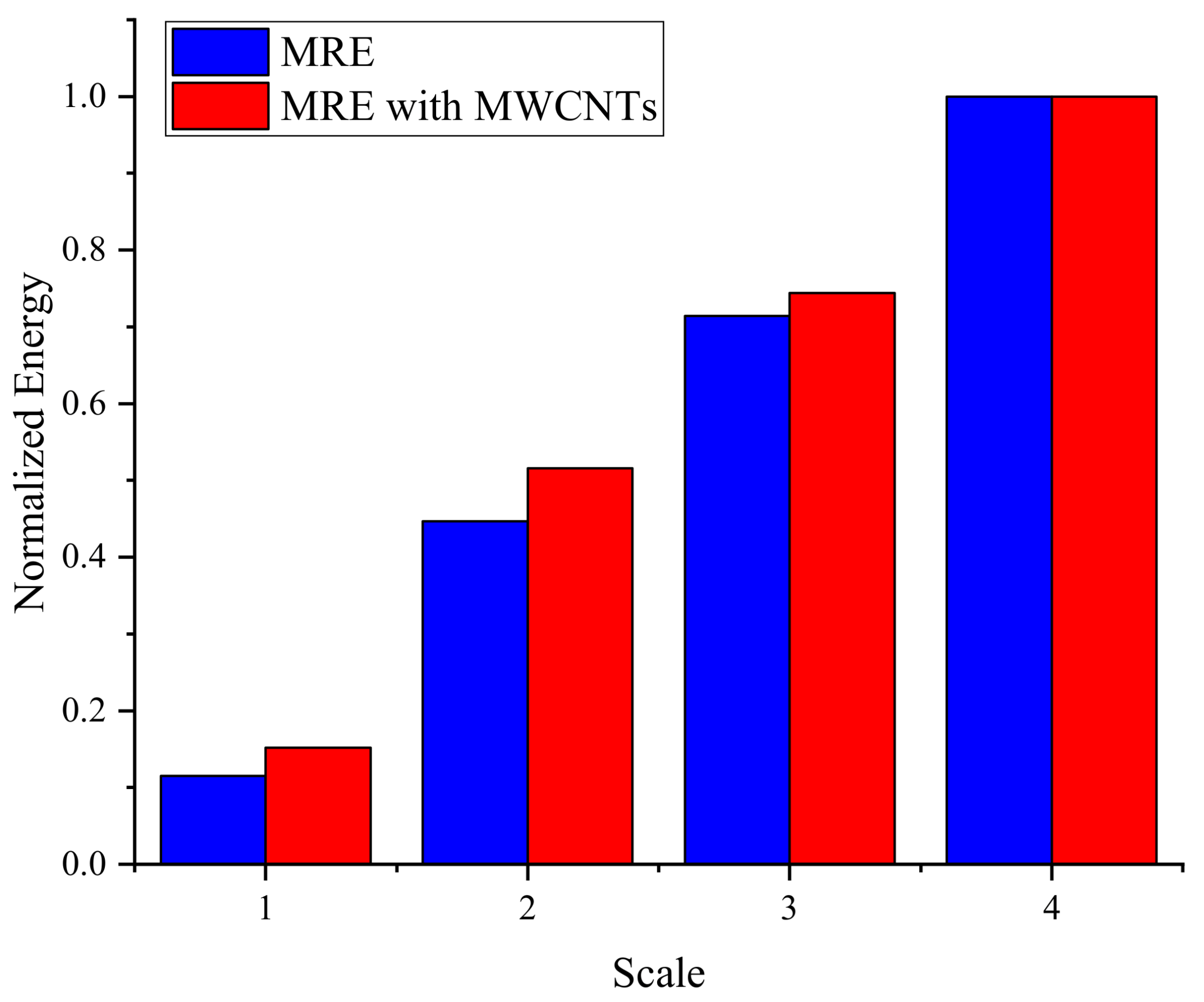
It can be seen from Figure 9 that the normalized energy distribution of curvelet coefficients at each scale is further studied by calculating the sum of squares of the amplitude of curvelet coefficients, denoted as: $E^{\left(a\right)}={\displaystyle \sum }_{b,\theta }^{}{\left|c\left(a,b,\theta \right)\right|}^2$.

Relative significance of each constituent of MRE or MRE with MWCNTs is measured at each scale. Scales 1 to 4 have an increasing trend of energy distribution. MRE with MWCNTs has relatively larger relative energy than MRE for almost all the scales. It indicates the importance of MWCNTs for function enhancement of MRE, since they change the energy distribution of curvelet coefficients.

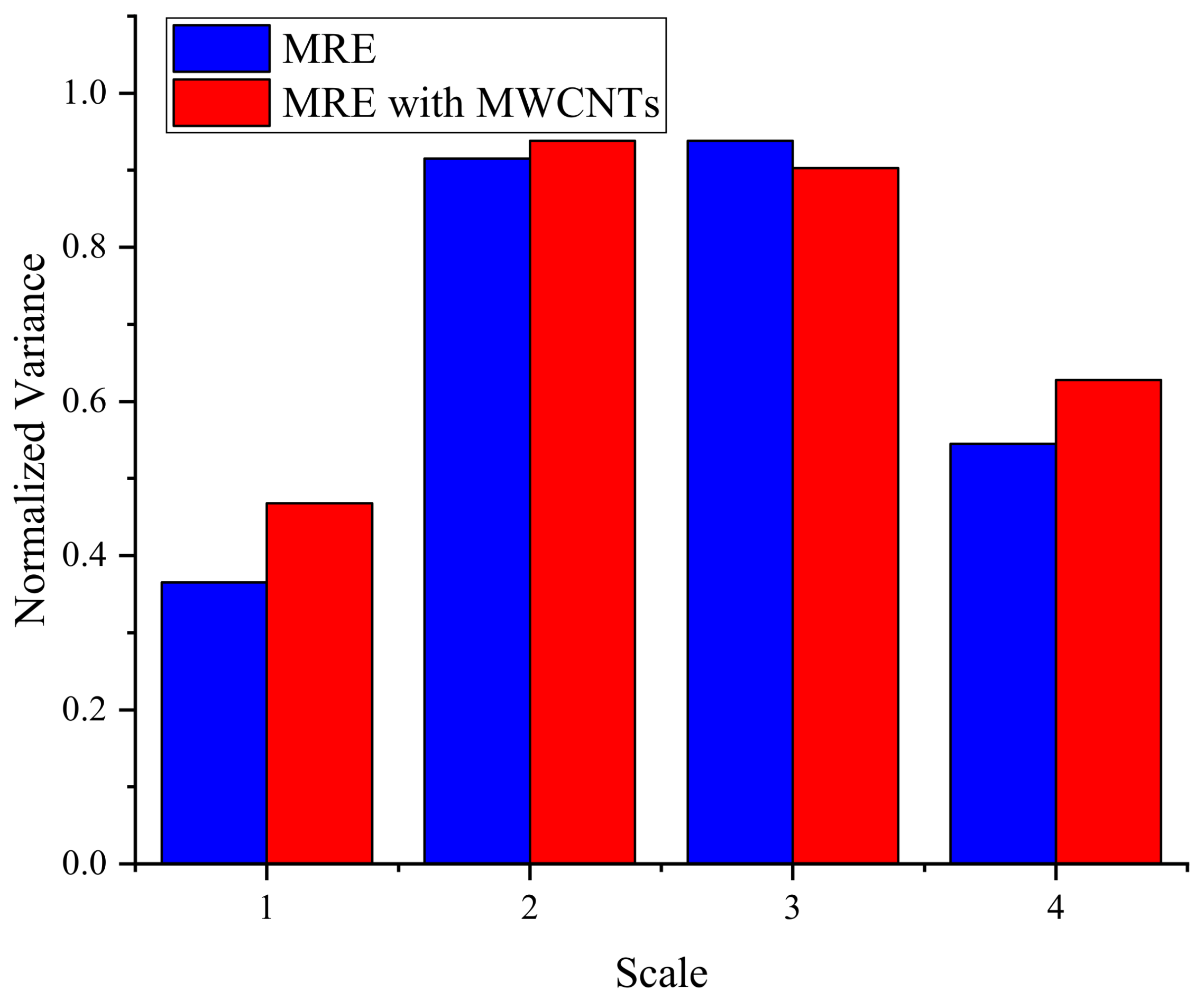
From Figure 10, it can be seen that, as the scale increases from one to four, the variance first increases and then gradually decreases. Large variance indicates the discrimination degree of energy concentration is relatively obvious along specific directions, angles or a few fractions of areas. Isotropic or stochastic characteristics of features are implied with smaller variance. This phenomenon is clearly reflected at scale four, where the energy variance is 0.62 for MRE with MWCNTs compared to 0.55 for MRE. The addition of MWCNTs renders the particles aligned in parallel and the composite more structured.

4. Design of an MRE-Based Adaptive Seismic Isolator

In this section a detailed description of an MRE-based adaptive seismic isolator (damper), including its attributes, characteristics, design and phenomenological behavior are discussed.

4.1. Design of Adaptive Seismic Isolator

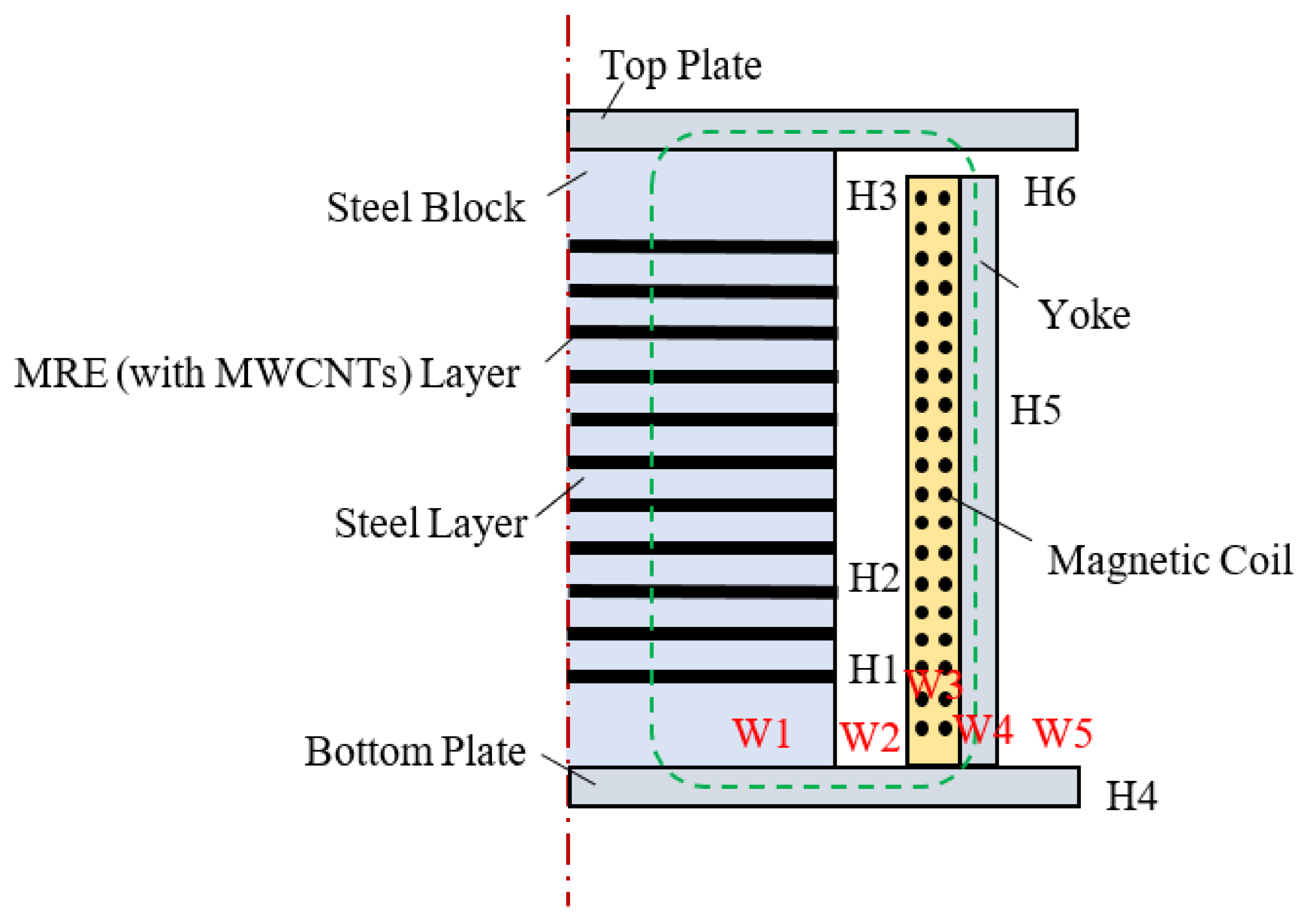
An innovative design of a magnetic circuit is explored with the aim of energizing the magnetic-induced isolator with novel MRE. By appropriately designing this new type of isolator system, enhanced loading–carrying ability is expected due to adaptive performance of variable stiffness and damping of novel MRE. Figure 11 shows a cross-section axis-symmetry sketch of a designed base isolator consisting of external yoke, top and bottom steel plates, magnetic coil, steel block, laminated MRE and steel layers.

The total device is a cylindrical structure, where smart MRE and steel layers are inside the magnetic coils. By applying current to the coils, the coils will produce a magnetic field and make the “smart laminates” coordinately work. When the system operates, the magnetic lines driven by energizing coils pass through the “smart laminates”, steel block, two steel plates and external yoke, which forms a closed loop shown by the dashed green line. The conductive steel layers are laminated between MRE layers and the steel blocks and are placed at the top and the bottom of the laminated structure. Due to the large volume of silicon rubber, magnetic conductivity of laminated MRE is relatively low while the steel layers have higher magnetic conductivity. Two steel plates at the top and bottom improve the overall magnetic conductivity. With this design, sufficient magnetic flux is guaranteed so that the overall magnetic conductivity and the permeability of the magnetic core are improved, and MRE layers perform superior damping performance. A gap between the top plate and the steel yoke is taken into consideration in that the inside laminate structure may have lateral and compressive deformation when the device is subjected to external loading [52].

Regarding component dimension, the radius of the inside laminate structure is W1 = 50 mm. The distance between the inside laminate structure and the coil is W2 = 12 mm. The thickness of the annular coil is W3 = 15 mm. The thickness of the yoke is W4 = 20 mm, and the length of the extended steel plate is W5 = 15 mm. The MRE magnetic-induced core has 50 layers with 49 bonded and laminated conductive steel layers. The thickness of MRE is H1 = 1.2 mm, and the laminated steel layer is H2 = 1 mm. The steel block between the plates and the laminate is H3 = 30 mm. The thickness of the top and the bottom plates is H4 = 10 mm. The magnetic coil has 3500 turns and is made of magnetic wire with a diameter of 1 mm, which is driven by a variable current excitation. The magnetic coil and annular yoke have the same height H5 = 164 mm. The gap between the top plate and the yoke is H6 = 5 mm.

4.2. Magnetic Circuit Analysis

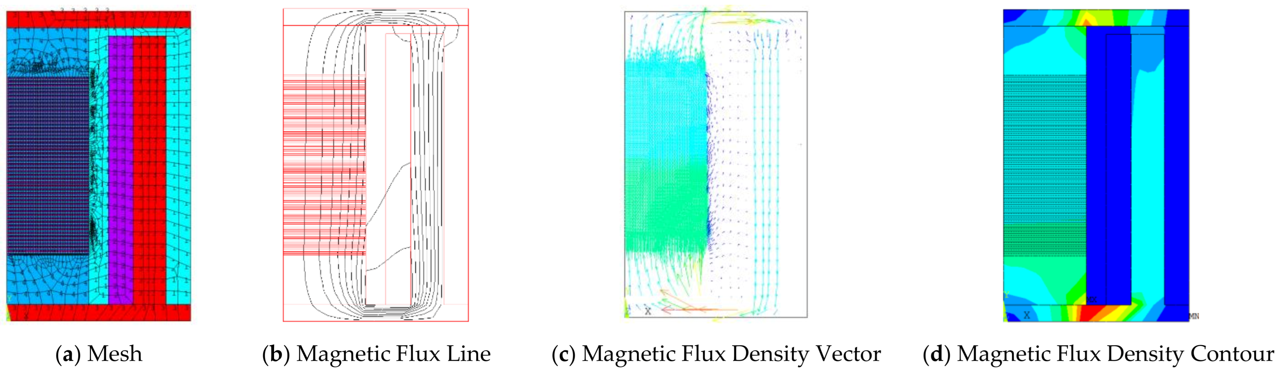
To study the magnetic circuit of the novel MRE isolator device, finite element analysis via ANSYS is carried out to simulate and illustrate the effectiveness and the reliability of this design. MRE models and their modified versions are used as isolator finite element model parameters by taking the effect of MWCNTs into account. Figure 12 shows the distribution of the magnetic flux inside the isolator when the applied current is 0.85: (a) is the smart mesh with mesh level 4 (1 denotes finest mesh and 10 represents coarsest mesh), (b) shows the distribution of the magnetic flux line, (c) is the magnetic flux density vector, and (d) is the contour plot of the magnetic flux density.

The maximum magnetic flux density is 0.799 T for MRE and 0.823 T for MRE with MWCNTs. The magnetic flux reaches strongest, both within the bottom plate, between steel block and yoke. The magnetic flux line passes through the yoke and magneto-rheological “smart layers”, which forms a closed loop. The strength of the magnetic flux density is relatively uniform within the “smart layers” and weakens both near the air and the edges of top and bottom plates. Based on this, the “smart layers” are designed in the center of the angular magnetic coil with steel laminates and steel blocks as a whole to increase the permeability. The key issue for designing the isolator is to form a stable, enclosed magnetic path with “smart” materials of high permeability. By optimizing the design structure, the energy loss of the magnetic field can be achieved at a reasonable level and in an efficient way. A comparative study for complete and incomplete design is conducted to study the importance of each part of the magnetic path.

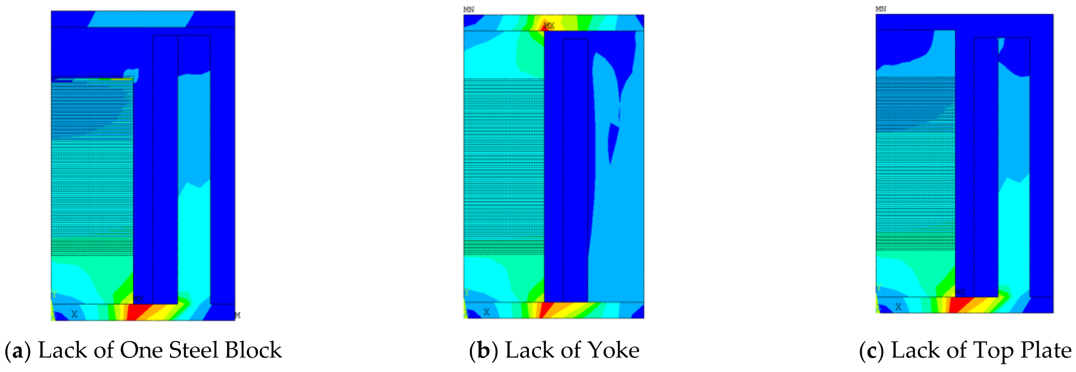
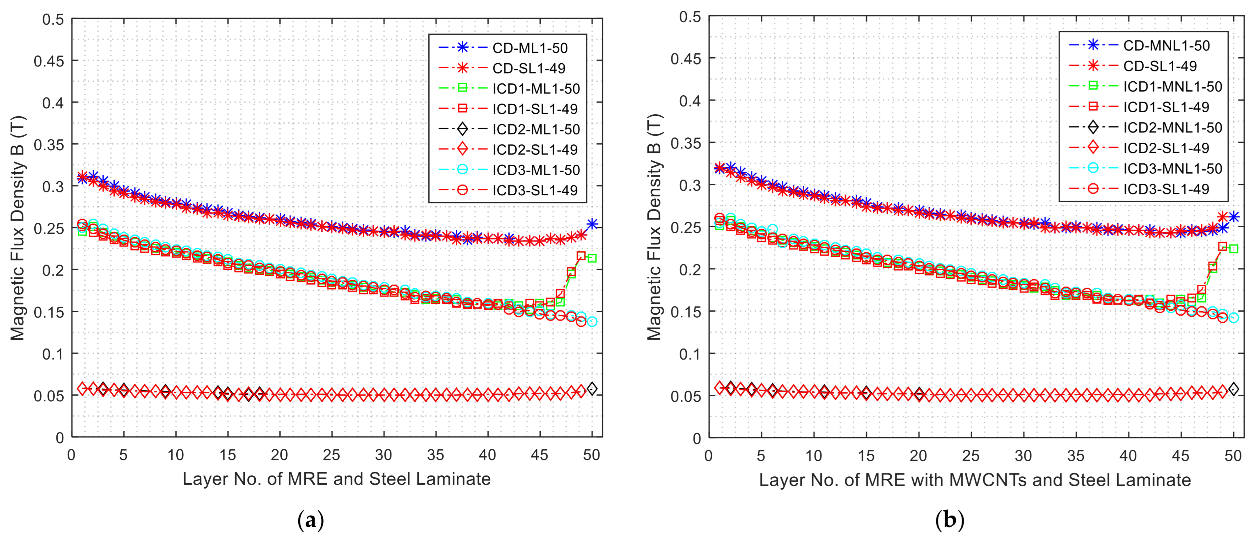
Figure 13 shows the distribution of the contour of magnetic flux density for incomplete design. For incomplete design, magnetic flux density at the missing part has a fast descending trend. The average value of the magnetic flux density of each “smart” layer (50 MRE, or MRE with MWCNTs, and 49 laminated steel sheets in total) is measured, with an external magnetic flux density of 0.85 T, and is shown in Figure 14. In this figure, CD is the complete design. ICD1, ICD2 and ICD3 represent incomplete designs without the upper steel block, yoke and upper steel plate, respectively.

ML denotes the layer of MRE, MNL denotes the layer of MRE with MWCNTs, and SL represents the steel sheet between laminated MRE. For all design schemes, the magnetic flux density has a descending trend. This is due to the fact that the gap between the steel yoke and the top plate increases the possibility of energy loss.

Thus, the closer the location is to the upper plate and the gap, the more magnetic energy is dissipated. For a complete design, with the layer of MRE or steel sheet increasing, the value of magnetic flux density decreases and weakens steadily. For all the areas of incomplete design, magnetic flux density dramatically decreases.

The maximum magnetic flux density for the incomplete design is about 0.255 T and 0.26 T for MRE laminate and MRE with MWCNTs laminate, respectively. Specifically, for ID1, the magnetic flux density first decreases and then has an abrupt rise. This is because the missing of upper steel block makes the magnetic flux redistributed and it concentrates the magnetic flux lines at the corner of the upper MRE layer. Therefore, a complete design of MRE core area is laminated with steel sheets together with steel blocks attached at the end of the laminated structure, which makes the magnetic flux circuit coherent as a whole. This design can also shift the weakening magnetic field away from the MRE laminate core area, and, at the same time, the narrow magnetic path between the yoke and the bottom plate makes the magnetic circuit have stronger connection.

4.3. Magnetic Distribution under Compressive and Shear Loading

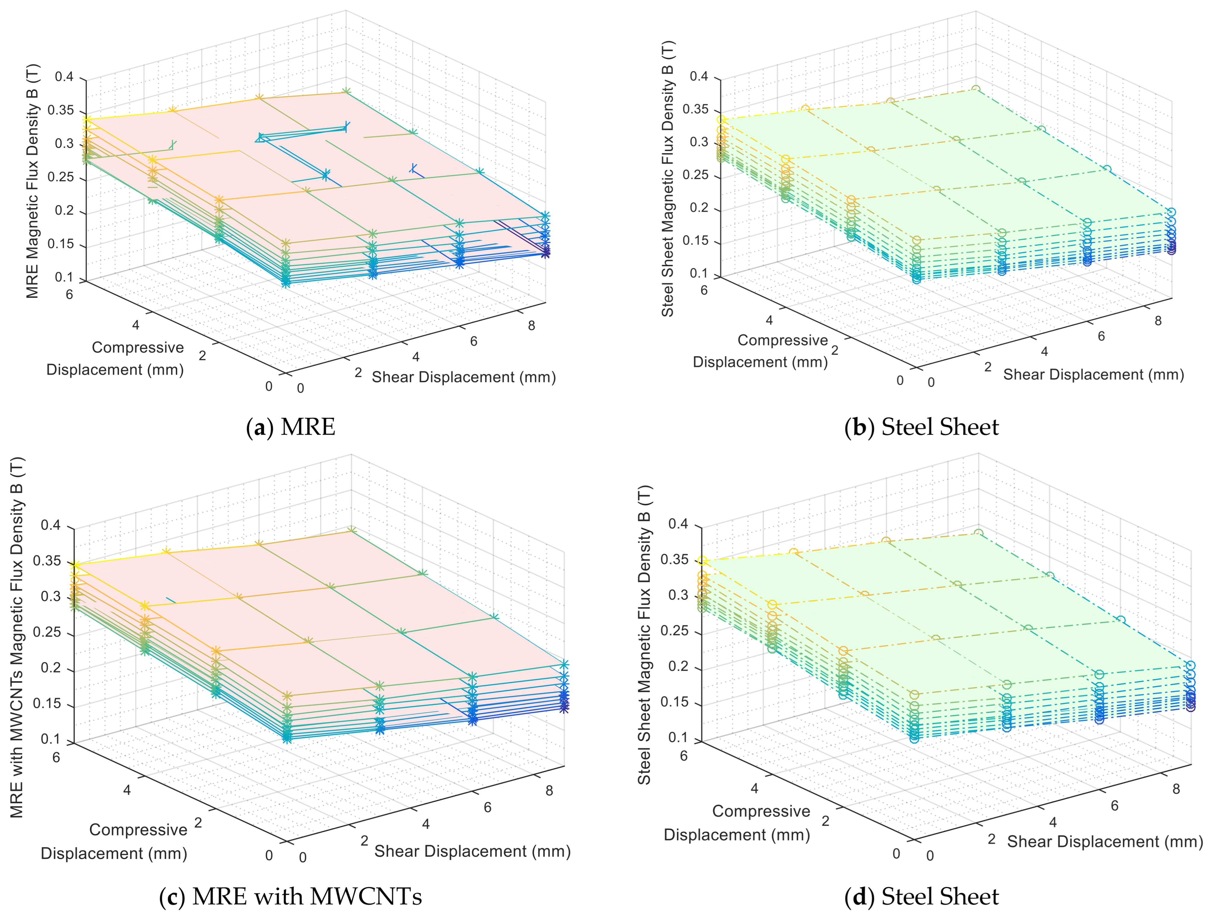
Magnetic field is sensitive to mechanical change or the motion of the device and it varies accordingly when external loading is applied. The location and the shape of MRE (or MRE with MWCNTs) layers may displace and change under compressive and shear loading. Under different shear (0 mm, 3 mm, 6 mm, 9 mm) and compressive (0 mm, 2 mm, 4 mm, 6 mm) displacement loadings, a comparative investigation of magnetic flux density is conducted for both MRE and MRE with MWCNTs. When the MRE (or MRE with MWCNTs) is sheared, Payne effect may occur as the strain achieves a threshold. When it is subjected to compressive loading, MRE (or MRE with MWCNTs) layers will approach the bottom plate where larger magnetic flux density occurs, and decreased distance between the magnetic dipoles increases the magnetic energy. In order to explain the relationship between strain and magnetic flux, a flux diagram of 5-layer MRE (or MRE with MWCNTs) are shown in Figure 15.

For both MRE (or MRE with MWCNTs) layers, the magnetic flux density has the largest value when the compressive displacement is 6 mm, and the smallest value when the shear displacement achieves 9 mm. This phenomenon agrees well with the aforementioned Model 5 of MRE.

Specifically, when the compressive displacement is 2 mm, with the shear displacement increasing from 0 mm to 9 mm, the magnetic flux density of layer 5 of MRE with MWCNTs decreases from 0.321 T to 0.262 T. This clearly demonstrates when the compressive effect is larger, the magnetic flux density increases. Both compressive and shear effects change the magnetic-induced structural state. The magnetic field decreases along with an increase in shear displacement and increases along with an increase in compressive displacement. Magnetic flux circuit is dependent on structural deformation and motion. It also shows that the larger the layer number of MRE (or with MWCNTs) or laminated steel sheet, the more magnetic energy loss happens due to the gap between the top plate and the yoke.

4.4. Suppressing Acceleration Effect

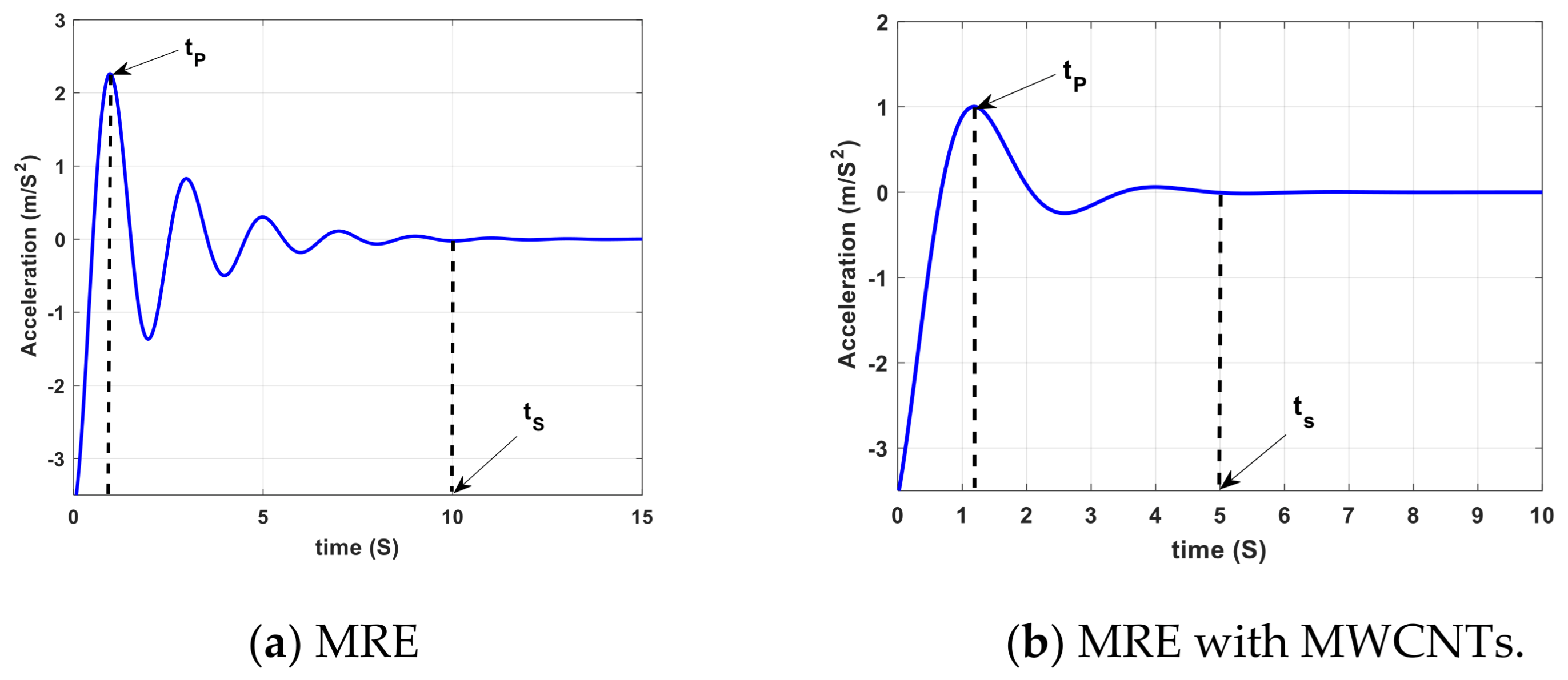
In order to illustrate the developed MRE idea in the paper, by employing mixing multiwall carbon nanotubes (MWCNT), Figure 16 is used to compare the suppressing acceleration response of MRE (or with MWCNTs).

As shown in the figure, the MRE has first peak amplitude, a number of peaks more than the MRE with MWCNTs, and settling time $t_S$ (the time required to eliminate the response peaks) equal to 10 and 5 s for MRE (or MRE with MWCNTs), respectively, also the peaks time $t_P$ (the time required to reach the first peak) equal to 0.9 and 1.16 s for MRE (or MRE with MWCNTs), respectively. It can be concluded that the MRE with MWCNTs has a suppressing acceleration effect superior to MRE.

5. Vibration Control of an Isolated Structure

Base isolated systems have been widely applied in civil infrastructure to protect buildings and bridges against earthquakes which result in ineffectiveness and malfunctioning of structural integrity as well as economic loss. The direct function of isolation system is to absorb dissipated energy from structural vibration caused by seismic wave, and isolate seismic motions from transmitting into main structure that may cause unpredicted damage. In the following sections the effectiveness of the proposed MRE-based Adaptive Seismic Isolator for vibration control in structural system is investigated.

5.1. Basic Principle of Structural Control

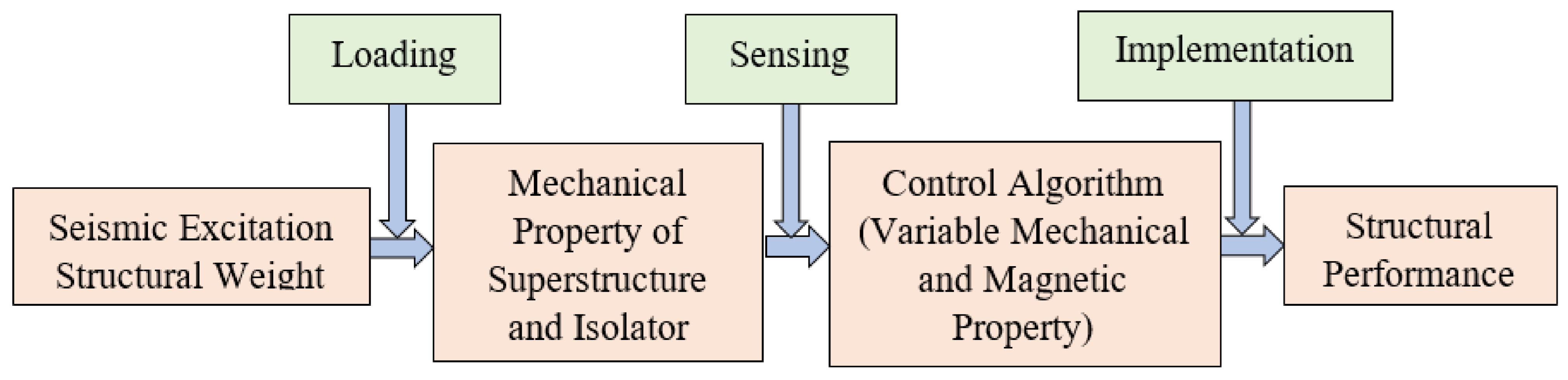
A scaled structural prototype model is built to verify and improve seismic mitigation performance. A base isolation device with a novel MRE (or with MWCNTs) is installed underneath the base to support the vertical upper loading, and at the same time to protect the building in case of lateral seismic shock. Laminated MRE can provide horizontal adaptive controllable flexibility as a smart base isolator while the steel sheets can provide adequate vertical loading capacity. Five viscoelastic models are incorporated to model the adjustable stiffness and damping properties of the “smart” isolator. When a seismic wave is approaching, online structural status is captured by the sensors installed on the structure, and the developed control algorithm is correspondingly applied to the isolation system, making it adaptively react to the changing structural status. At the same time, a changing magnetic field is generated across the isolation device which tunes the stiffness and damping properties of the smart material that reacts to external disturbances. Thus, the structure can be well controlled with the developed control algorithms and the smart material. This process is clearly depicted in Figure 17.

Assuming that a typical state-space form of a $\left(n+1\right)$ degree of freedom structure is expressed as the following structural dynamics expression:

$$M\ddot{x}\left(t\right)+C\dot{x}\left(t\right)+Kx\left(t\right)=Pu\left(t\right)+Qw\left(t\right)$$

(16)

where $x\left(t\right)={\left[x_n, x_{n-1},\cdots ,x_1,x_b\right]}^T$ represents the $\left(n+1\right)$ order vector, and $x_i$ is the displacement of the ith floor. $M$,$K$,$C$ are $\left(n+1\right)\times \left(n+1\right)$ mass matrix, stiffness matrix and damping matrix, respectively, and $m_i$, $k_i$ and $c_i$ are the corresponding elements of mass, stiffness and damping matrix. Specifically, $k_{isl}\left(t\right)$ and $c_{isl}\left(t\right)$ are stiffness and damping coefficients of the smart base isolator, respectively.

$$M=\left[\begin{array}{c}{m}_n \\ m_{n-1} \\ \ddots \\ m_1\end{array}\right]$$

(17)

$$K=\left[\begin{array}{c}{k}_n -k_n \\ -k_n k_n+k_{n-1} -k_{n-1} 0\\ \ddots \ddots \ddots \\ 0 -k_2 k_2+k_1 -k_1\\ -k_1 k_1+k_{isl}\left(t\right)\end{array}\right]$$

(18)

$$C=\left[\begin{array}{c}{c}_n -c_n \\ -c_n c_n+c_{n-1} -c_{n-1} 0\\ \ddots \ddots \ddots \\ 0 -c_2 c_2+c_1 -c_1\\ -c_1 c_1+c_{isl}\left(t\right)\end{array}\right]$$

(19)

In Equation (16), $P$ and $Q$ respectively represent $\left(n+1\right)\times m$ location matrix of the control force and $\left(n+1\right)\times s$ location matrix of the external loads, $u\left(t\right)={\left[u_1, u_2,\cdots ,u_m\right]}^T$ and $u\left(t\right)={\left[u_1, u_2,\cdots ,u_m\right]}^T$ are respectively a vector of $m$ control forces and $s$ external environmental loads or disturbances. The state space equation of Equation (16) is expressed as follows:

$$\dot{z}\left(t\right)=Az\left(t\right)+Bu\left(t\right)+Ew\left(t\right)$$

(20)

where $z\left(t\right)={\left[z_1, z_2,\cdots ,z_{2n+2}\right]}^T$ is a $\left(2n+2\right)$ state vector, $A$ is a $\left(2n+2\right)\times \left(2n+2\right)$ system matrix, $B$ is a $\left(2n+2\right)\times m$ control matrix and $D$ is a $\left(2n+2\right)\times s$ disturbance matrix. These have the following forms:

$$z\left(t\right)=\left[\begin{array}{c}x\left(t\right)\\ \dot{x}\left(t\right)\end{array}\right]$$

(21)

$$A=\left[\begin{array}{c} 0 I\\ -M^{-1}K -M^{-1}C\end{array}\right]$$

(22)

$$B=\left[\begin{array}{c} 0 \\ M^{-1}P\end{array}\right]$$

(23)

$$E=\left[\begin{array}{c} 0 \\ M^{-1}Q\end{array}\right]$$

(24)

Herein, some parameters are assigned as follows: $m_3=m_2=m_1=m_b=10 \mathrm{kg}$, $k_3=k_2=k_1=100$, and $c_3=c_2=c_1=50$, $P=Q={\left[0 0 0 1\right]}^T$ means the control force and the external excitation are applied at the bottom floor, $k_{isl}\left(t\right)$ and $c_{isl}\left(t\right)$ are stiffness and damping coefficients, which can be scaled and assigned according to the five MRE models and their modified models.

5.2. Reaching Law-Based Sliding Mode Control

Sliding mode control is particularly suitable for semi-active control of both linear and nonlinear variable-stiffness structural systems [53]. In general, the dynamic system can be considered as:

$$\dot{z}\left(t\right)=Az\left(t\right)+Bu\left(t\right)+d\left(z,t\right)$$

(25)

where $d\left(z,t\right)$ represents the external system disturbances regarding $Ew\left(t\right)$. $\delta \left(z,t\right)$ is the upper bound of the disturbance satisfying $\Vert d\left(z,t\right)\Vert \le \delta \left(z,t\right)$. The tracking error of the system is:

$$e=z-z_d$$

(26)

The goal of vibration control is to meet $z_d=0$ and then $e=z-0=z$.

The basic design of the sliding mode control includes two stages. In the first step, a hyperplane $s\left(e\right)$ is chosen to describe the dynamic behavior of the control system. The second step includes designing a controller such that the trajectory of the system converges to, and always remains on, the sliding surface. $m$ switching functions are chosen as follow

$$s\left(z\right)=rz$$

(27)

$$s_i\left(z\right)=r_{i}z=r_{i1}{z}_1+r_{i2}{z}_2+\cdots r_{i2n+2}{z}_{2n+2} i=1,2,\cdots m$$

(28)

where $s$ is a $m\times 1$ vector, and $r={\left[r_1,r_2,\cdots ,r_m\right]}^T$ is a $m\times \left(2n+2\right)$ vector, and $r_i=\left[r_{i1},r_{i2},\cdots ,r_{i2n+2}\right]$, $r_i$ is a sliding vector. In the sliding mode control, the system satisfies $s\left(z\right)=0$ and $\dot{s}\left(z\right)=0$, and the control force is called the equivalent control force, i.e.,

$$u_{eq}=-{\left(rB\right)}^{-1}\left(rAz+rEw\right)$$

(29)

Thus, the control law can be chosen as:

$$u=u_{eq}+u_h$$

(30)

External excitation term $d\left(z,t\right)$ can be dropped from Equation (29). Therefore, the equations governing the system dynamics may be acquired from the following design.

$$u_{eq}=-{\left(rB\right)}^{-1}rAz$$

(31)

The exponential reaching law can be expressed as:

$$u_h=-{\left(rB\right)}^{-1}\left[\eta sgn\left(s\right)+gs\right] \eta >0, g>0$$

(32)

5.3. RBF Based Adaptive Sliding Mode Control

The biggest advantage of RBF adaptive control is that the unknown nonlinearity of the system can be approximated by an RBF neural network whose weight value parameters are adjusted according to the adaptive law for the purpose of controlling the nonlinear system to track a given trajectory. Let’s consider a system derived from Equation (20).

$$\dot{z}\left(t\right)=f\left[z\left(t\right)\right]+Bu\left(t\right)+Ew\left(t\right)$$

(33)

Matrix $Az\left(t\right)$ is replaced by a term $f\left[z\left(t\right)\right]$ that considers both changing stiffness and damping properties of the system. The magnetic circuit has been studied to conclude that the “smart” base isolator can be adjusted when the system is subjected to an external uncertainty such as an earthquake [54,55,56]. Thus, an adaptive control law can be designed to meet the system uncertainty and the requirement of system adaptability. Defining the sliding mode function as:

$$s\left(z\right)=re+\dot{e}, \mathrm{Then}$$

(34)

$$\dot{s}\left(z\right)=r\dot{e}+\ddot{e}=r\dot{e}+f\left[z\left(t\right)\right]+u-{\ddot{z}}_d$$

(35)

RBF neural network has its superiority in its good approximation capability to any unknown function. The algorithms of RBF networks are:

$$h_j=exp\left(\frac{\Vert z-c_j{\Vert }^2}{2b_j^2}\right)$$

(36)

$$f=W^{\ast T}h\left(z\right)+\epsilon$$

(37)

where $z$ is the input signal of the network, $j$ is the number of hidden layer nodes in the network, $h={\left[h_1,h_2,\cdots ,h_n\right]}^T$ is the output of the Gaussian activation function, $W^{\ast }$ is ideal neural network weight value, and $\epsilon$ is the approximation error that satisfies $\epsilon \le {\epsilon }_N$. $f\left[z\left(t\right)\right]$ can be approximated by an RBF neural network defined as:

$$\widehat{f}\left(z\right)={\widehat{W}}^{T}h\left(z\right)$$

(38)

Thus, the control law can be expressed as:

$$u=\frac{1}{B}\left[\widehat{f}\left(z\right)+{\ddot{z}}_d+mE\right]$$

(39)

where $m$ is a parameter with respect to system errors, $E={\left(e, \dot{e} \right)}^T$.

The adaptive law is expressed as:

$$\widehat{W}=-\gamma E^{T}Pbh\left(x\right)$$

(40)

where $P$ is a parameter with respect to Lyapunov stability analysis.

5.4. Comparison of Different Control Schemes

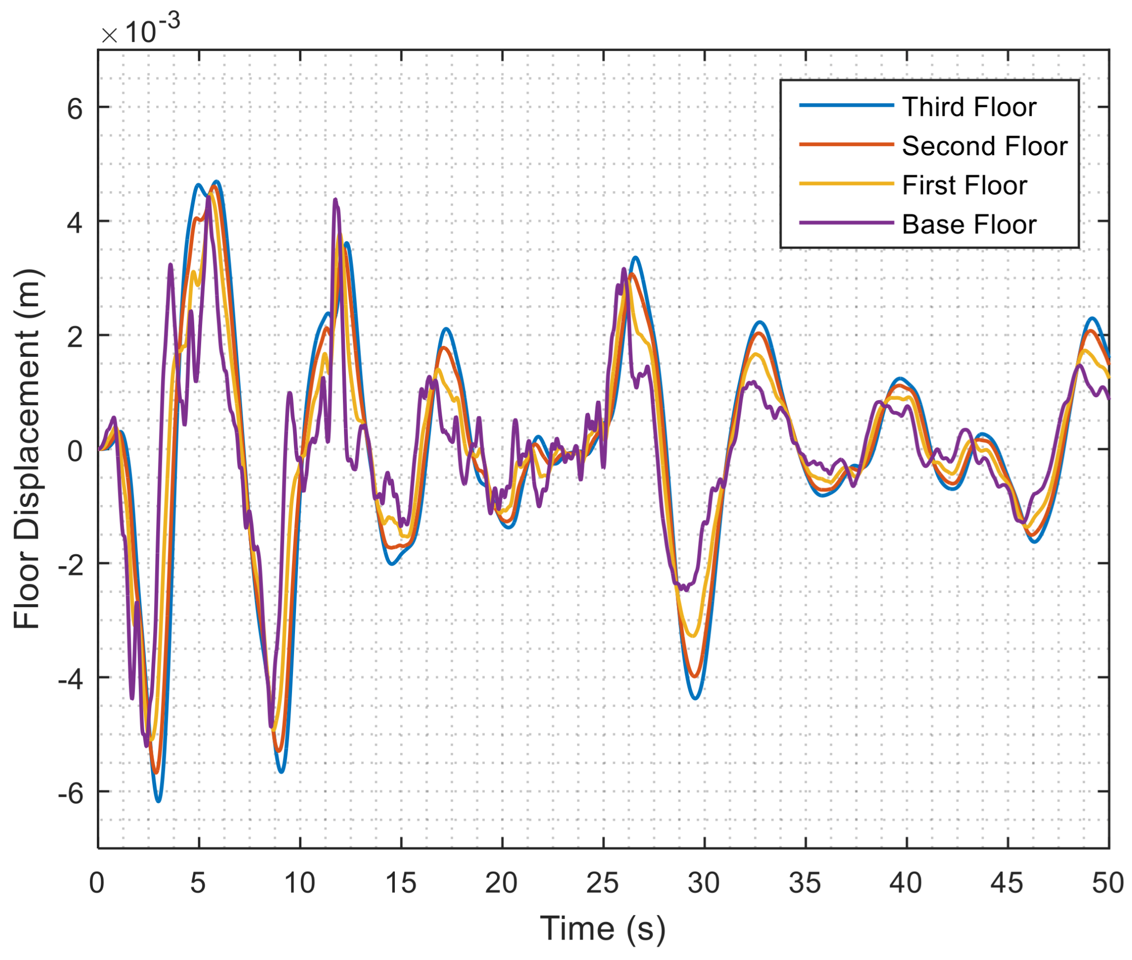
The developed adaptive seismic isolator can provide stable and reliable magnetic field to enable a controllable structure by energizing field-dependent MRE. The goal for the implementation of control algorithms is to make the isolator dissipate large energy and keep floor displacements stable and within the desired thresholds. Figure 18 shows the displacement of different floors without control. It is observed that in spite of the base floor, the third floor has maximum displacement and the first floor has relatively smaller displacements.

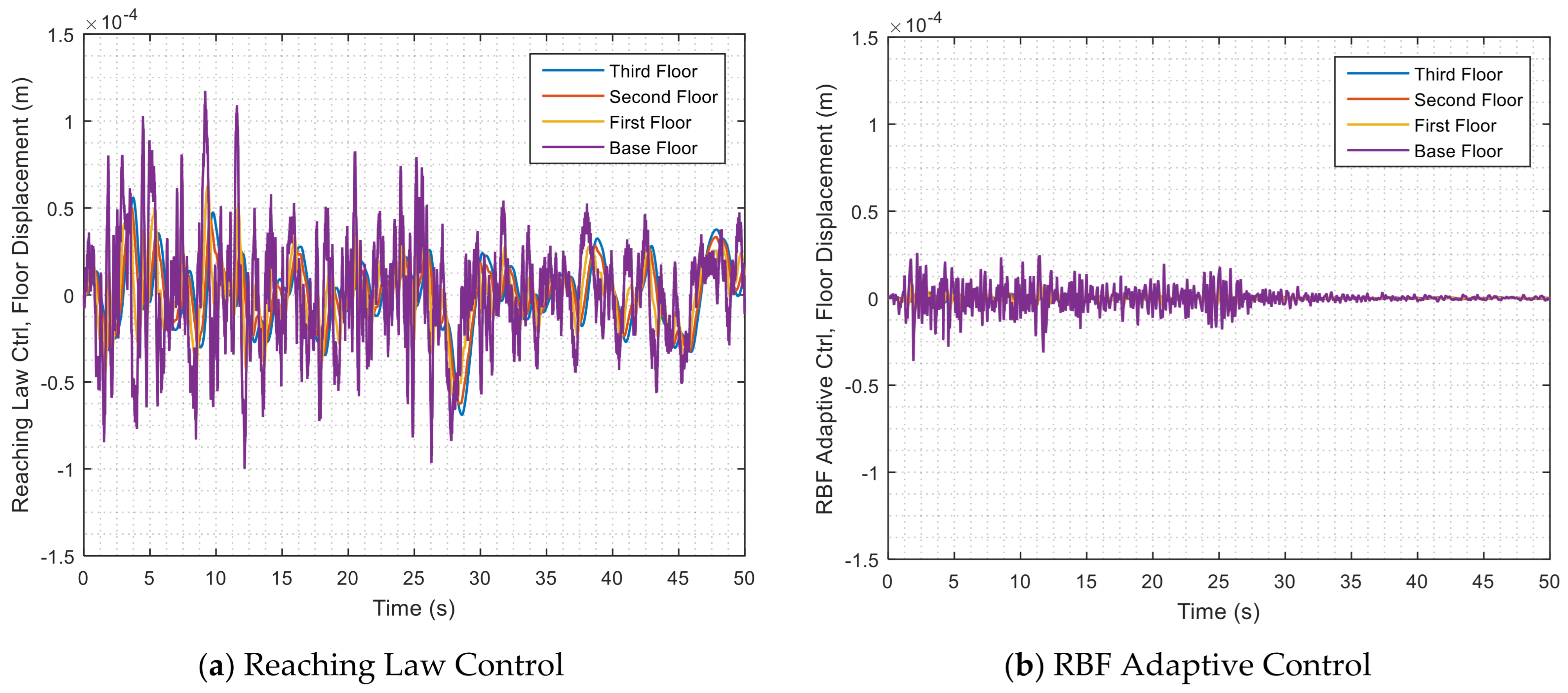
Figure 19a,b shows the structural displacement of each floor with the implementation of reaching law-based sliding mode control and RBF-based adaptive sliding mode control by incorporating modified M5 which describes the mechanical and magnetic characteristics of MRE nanocomposite. Compared with the displacement amplitude of Figure 19a,b, it can be seen that the displacement of the all floor is controlled due to the installation of RBF adaptive isolator.

Figure 20 shows the corresponding control forces applied to the structure when implementing these two schemes. Structural nonlinear performance has a strong relationship with the designed MRE-based variable stiffness and damping isolator and the developed control algorithms. The main disadvantage of the sliding mode control includes high frequency oscillation, which is called “chattering”. For the reaching law-based control method, the chattering phenomenon is obvious, while with the development of adaptive control algorithm based on the RBF model, the chattering effect is dramatically decreased.

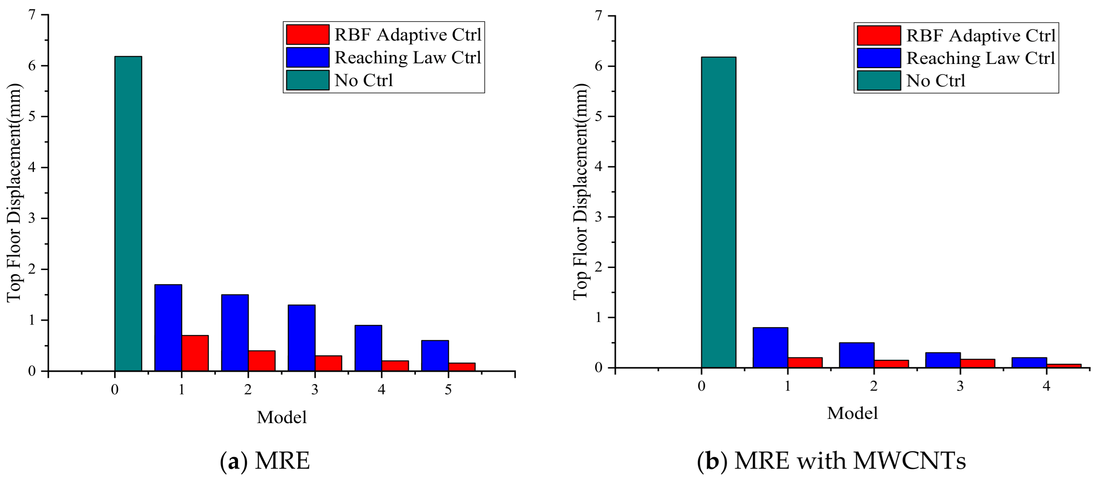
Figure 21 shows top floor displacement in different control schemes. Figure 21a, No. 0 represents no control effect. No. 1–5 represent Model 1–5 (MRE) applied to reaching law-based sliding mode control scheme, and (MRE) applied to the RBF adaptive sliding mode control method.

Figure 21b is the application of for MRE with MWCNTs. It can be seen that the maximum floor displacement without control dramatically decreases when implementing the two control schemes. RBF adaptive control shows its superiority over reaching law-based control due to its better controllability. These results also demonstrate the exceptional behavior of novel MRE nanocomposites for energy dissipation and vibration suppression of structural dynamics when applying them on isolation devices. For other Modified Models, similar cases occur but the reduced amplitude is slightly smaller than that of the Modified M5.

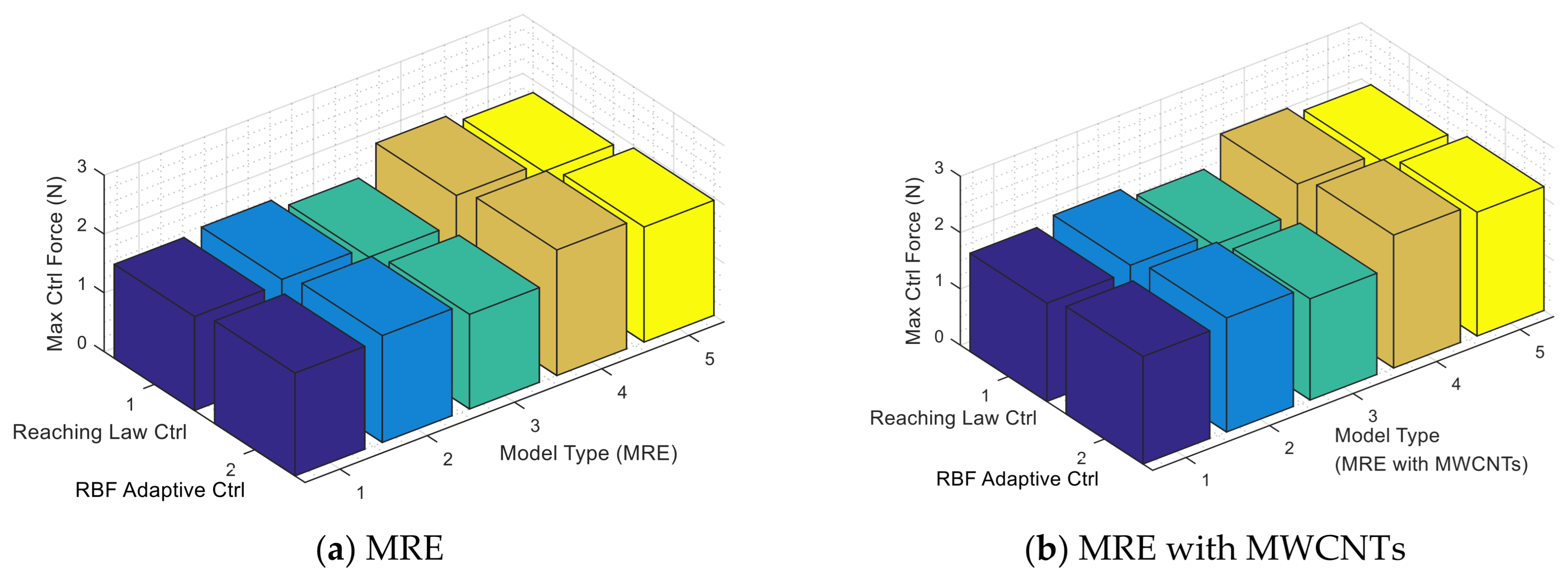
Figure 22 shows the maximum control force applied to the nonlinear structural system when applying different viscoelastic models. The control force is improved by 11.05% when using MRE nanocomposite compared with traditional MRE. Compared with reaching law-based control, RBF adaptive control shows its superior and improved controllability for about 8.63%. This is due to its online adaptability to track the changing trajectory of the system response with high nonlinearity. These phenomena also demonstrate the energy dissipation capability of the “smart” laminated MRE nanocomposite in the damping device, which suppresses the structural vibration during operation.

5.5. Adaptability, Controllability and Nonlinearity

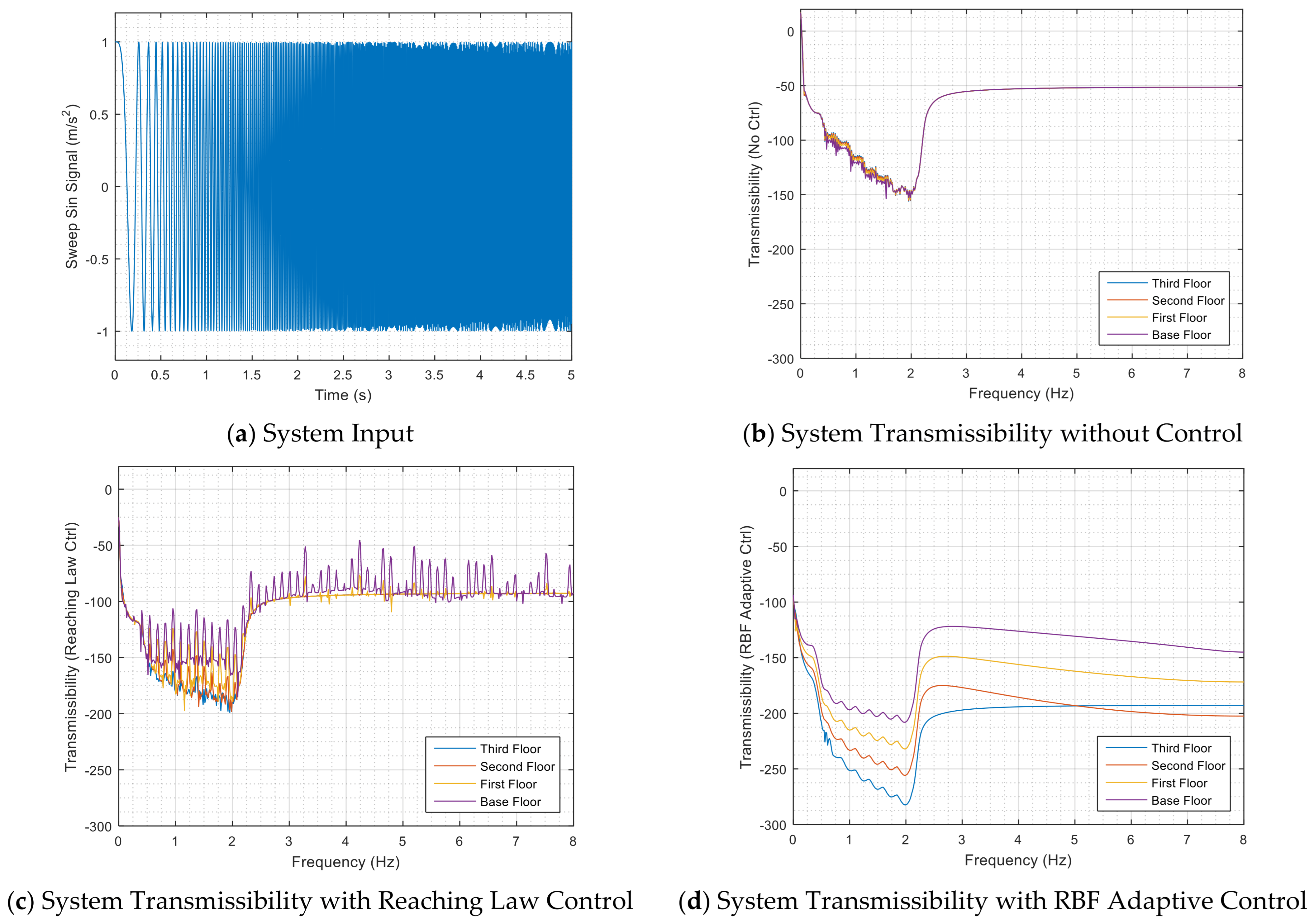
With the implementation of “smart” magnetorheological elastomers, an adjustable broadband frequency-tunable isolator can provide adaptability of natural frequency for real-time vibration control against non-stationary disturbance. In order to evaluate the controllability of MRE isolator with developed control algorithms, a sweep sine wave is used to excite the structure. Acceleration transmissibility is calculated to measure the effectiveness of vibration mitigation. Considering high nonlinearity of the material of the isolator, structural system and the control system, system transmissibility is used to assess the controllability of the structure.

Taking Model 5 as an example, sweep sine wave is used as the input signal and the responses of different floors are regarded as output signals. The sweep sine signal has a changing frequency ranging from 0 Hz to 150 Hz at the end of the excitation signal. Sampling rate is chosen to be 1000 Hz. Figure 23 shows the relationship between the system transmissibility function and the system frequency. All transmissibility functions indicate the intrinsic of the structural system is within 0–2 Hz. For the structure without control, the transmissibility functions of all floors are almost similar, which means that the structural integrity is good. But for the structure with control, the transmissibility functions differentiate from one to another. This illustrates good controllable performance of the structure. For reaching law-based control, chattering is also obvious, which can be inferred from the transmissibility of the base floor. Although the control forces adaptively change according to the magnitude of the excitation, they change slightly slow and gradual. Thus, former excitation has a lasting and longer influence on the subsequent structural dynamic response. For the RBF based control, the transmissibility functions between different floors are very smooth but separate.

This type of control is modeled by replacing the system matrix with an RBF approximation in the state space expression. The system response with the RBF adaptive control almost simultaneously follows the seismic excitation, showing a good control performance and control effect.

This demonstrates when the excitation is applied to the structure, the structure can react to the excitation quickly and adaptively with the developed adaptive control scheme. Large transmissibility values indicate better controllability which reduces the responses of the superstructure to a minimum. At the same time, energy can be absorbed and dissipated by designing the “smart” MRE isolation system appropriately. Most importantly, external non-stationary and uncertain disturbances are well “absorbed” by designing the RBF adaptive control scheme together with the isolator with the novel MRE material.

6. Conclusions

This paper first studies five parametric models of a traditional magnetorheological elastomer and modifies them by taking into account an incorporated functionally enhanced nanocomposite additive. Later, a novel curvelet approach is proposed for the identification of “smart” magnetorheological elastomeric material in a microscopic level. A curvelet transform keeps the characteristics of adaptive time-frequency window and multiresolution analysis which wavelet possesses, but extends these properties with varying identification angles. This property shows its superiority to make a thorough investigation on both approximate and detailed proportions of materials. By making use of this advantage, magnetorheological elastomer is found to be more functionally effective when it is mixed with multiwall carbon nanotubes. Later, a comparative study on complete and incomplete designs of an isolator with this novel MRE is conducted to show an optimal magnetic circuit design. This isolation device is further tested numerically to discuss and investigate the magnetic distribution under both compressive and lateral loading.

Finally, a comparative study between the traditional reaching law-based sliding mode control and an RBF adaptive sliding mode control scheme is carried out based on a prototype structural model with the designed novel MRE isolator. It is prove that RBF adaptive control method can consider the nonlinearity of the structural system, and can react to external disturbances adaptively with perfect controllability. Overall, this paper provides an idea, technique and methodology to verify how a novel and “smart” isolation system is developed regarding material fabrication, model expression, isolator design evaluation and control algorithm application. Future work will focus on incorporating the Bouc-Wen-Baber-Noori (BWBN) hysteresis model into the nonlinear structural dynamics. The experimental work will be conducted on magnetic circuit analysis, design of MRE isolator, and verification of robustness of control algorithm effectiveness for a scaled prototype structural model.