Evaluation of Unfilled Sheath in Concrete Structures Using Response Waveform in Time Domain

Abstract

The impact elastic wave method (IEW) has been applied to evaluate the thickness and internal defects of the target structure based on the dominant frequency of the response wave that is formed by the repeated reflections in the thickness direction. However, it is difficult to evaluate the size and position of the defect by IEW if the size and depth are relatively small and deep, respectively, and further, it is known that the technique is inapplicable if the target is not a plate-like structures. Therefore, the authors propose a new technique that uses Difference value as a new evaluation index to overcome the limitations of the conventional methods. Difference value shows the change of the response waveform in the time domain; it is computed by using a response waveform of the structures in sound condition as a reference. In this paper, the practicality of the Difference value is investigated by performing experiments using concrete specimens. The results of the experiments demonstrate that Difference value changes by the influence of internal defects, and Difference value evaluates the location of the relatively small defect that is difficult to evaluate by the conventional technique.

1. Introduction

1.1. Non-Destructive Testing for Concrete Structures

Concrete is one of the most common construction materials. It is widely used for the construction of structures because the unit price of materials is low and on-site construction is easy [1]. For the asset management of the concrete structures, quality control during the construction and maintenance after the construction are significant roles. The soundness evaluations are performed for the objectives, and the results are used for the preventive maintenance as well. Although the visual inspection and hammering test are frequently conducted for the soundness evaluation, the techniques investigate only the surface of the structures, and it is difficult to evaluate the internal condition. In addition, it is known that the results of these techniques depend on the ability of the inspector. Hence, the results of the investigations might be unreliable if the inspector is unskilled. Therefore, the use of NDT and micro-destructive test are considered in order to guarantee the accuracy of the investigations [2,3].

The IEW method is one of the NDT techniques of concrete structures [4,5,6,7,8,9,10,11,12,13,14,15,16,17,18,19,20,21,22,23,24,25]. It has been applied to evaluate the thickness and internal defects of the target structure based on the dominant frequency of the response wave that is formed by the repeated reflections in the thickness direction. Furthermore, it is suitable for testing concrete structures because the frequency of the excitation is relatively low, and the elastic wave emitted by the excitation is not easily attenuated [4,8]. In the field of NDT of concrete structures using IEW, Sansalone et al. [4,5,6]. elucidated the response characteristics of elastic waves in the concrete structures and established a method to evaluate the thickness and internal defects of the concrete structures based on the frequency of standing waves that are formed by the reflection of the elastic waves in the structures [4,5,6,7,8,9,10]. The elastic wave is reflected at a boundary where the acoustic impedance changes discontinuously. As a consequence, standing waves are formed between the boundaries, and the dominant frequency of the standing waves is determined by the distance between the boundaries. If the structure is sound, the boundaries are the surfaces of the structure and the dominant frequency is determined by the thickness of the structure. On the other hand, if the structure has internal defects, the boundaries are the surface of the structure and internal surface at the defect, and the dominant frequency is determined by the depth of the defect as a consequence. This evaluation method is called “Impact-Echo”, and research on this technique has been actively conducted [12,13,14,15,16,17,18,19,20,21,22,23,24,25]. However, generally speaking, evaluation using Impact-Echo would be difficult if the size of the defect is relatively small or the location of the defect is deep since the multiple reflections are not formed clearly under the conditions [7,21]. Further, if the structures are not able to be considered plate-like structures, it is difficult to apply the Impact-Echo because standing waves are not formed between the surfaces [22,23,24,25]. The configuration of the plate-like structures in which Impact-Echo is applicable is defined in “ASTM-C1383-04” [26]. According to the definition, the lateral dimensions are at least six times the thickness so that the standing waves are correctly formed in the thickness direction. On the other hand, Lin and Sansalone proposed a technique that evaluates the internal defects in the members of a rectangular cross-section [22,23]. This technique evaluates the soundness by using changes of the frequency characteristic of the members of the same configuration. However, if applied to existing structures, the evaluation indexes are the frequency characteristics of the members considered to be sound, and there is no guarantee that these indexes are sound. Consequently, it is not necessarily that the result shows the defects.

For overcoming these difficulties, a new evaluation method called Differential Value Analysis (DVA) is proposed in this paper. In DVA, Difference value, defined as the change of the waveform in the time domain, is used as an index to evaluate the soundness of the structures. The proposed method is validated experimentally by performing the model tests with concrete specimens in which unfilled sheaths are embedded. Furthermore, IEW and DVA are applied to the experimental results, and the capability of the proposed method.

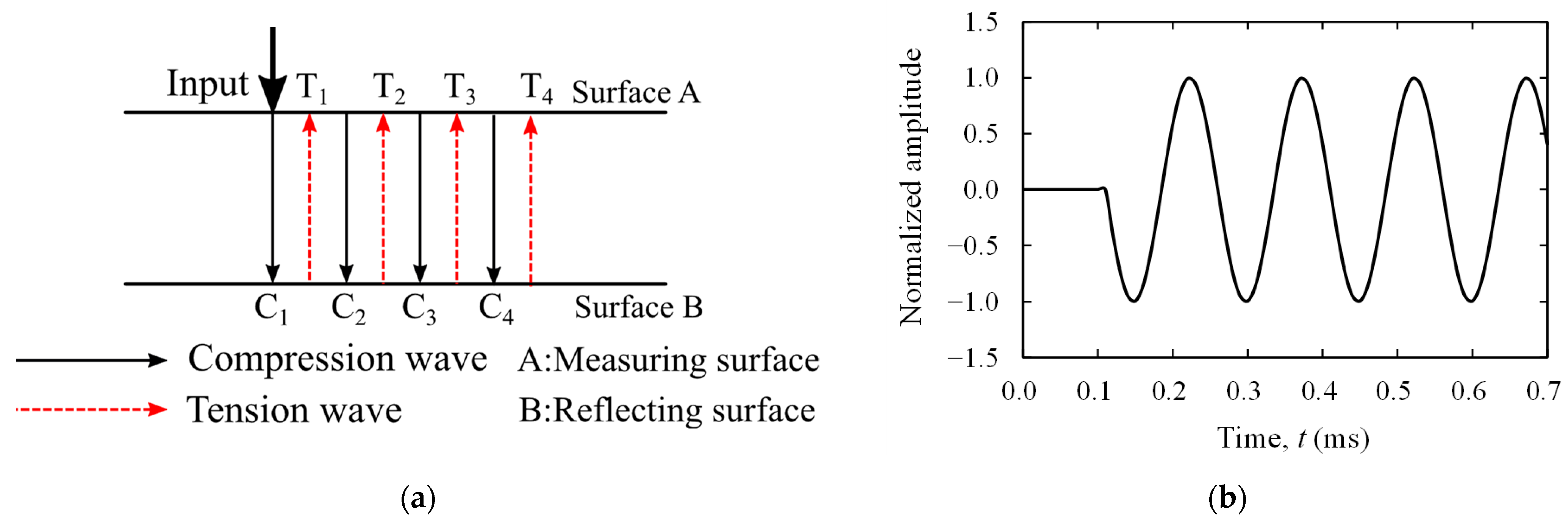
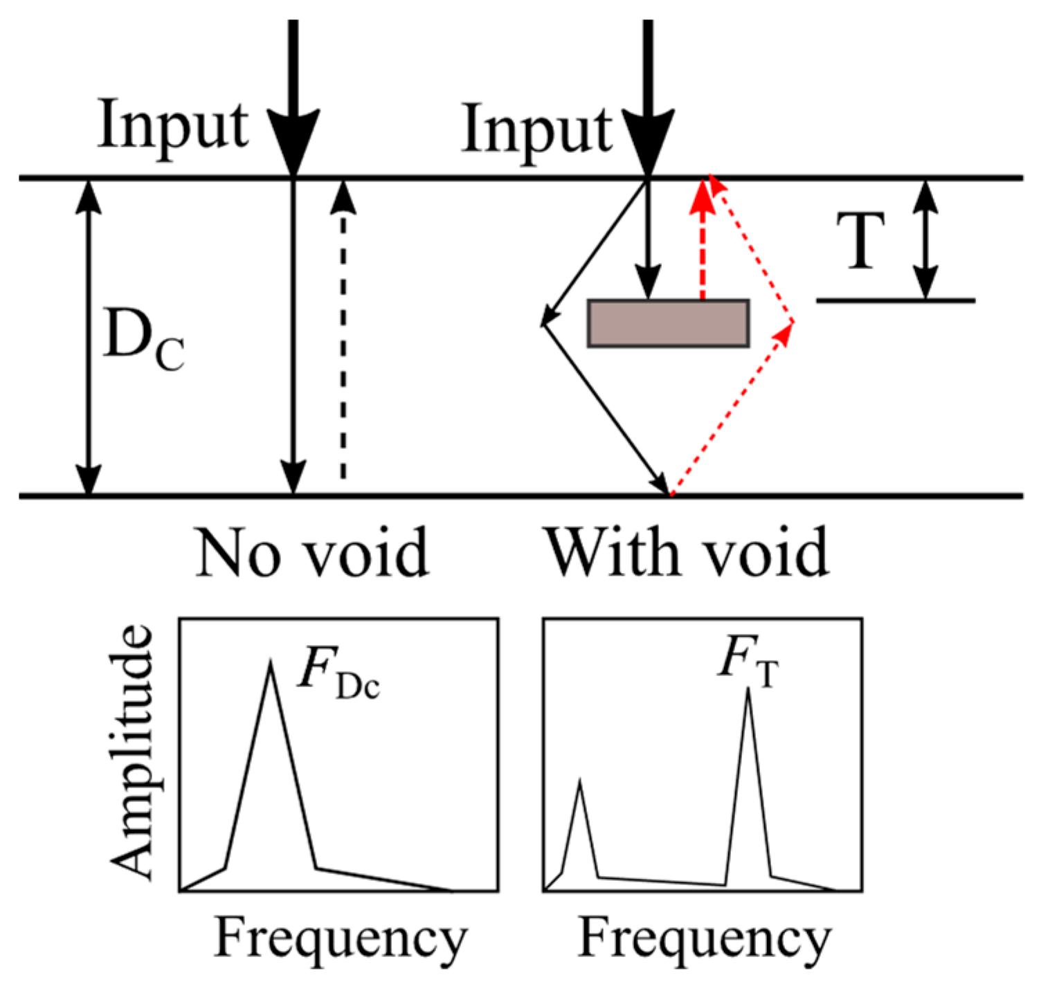
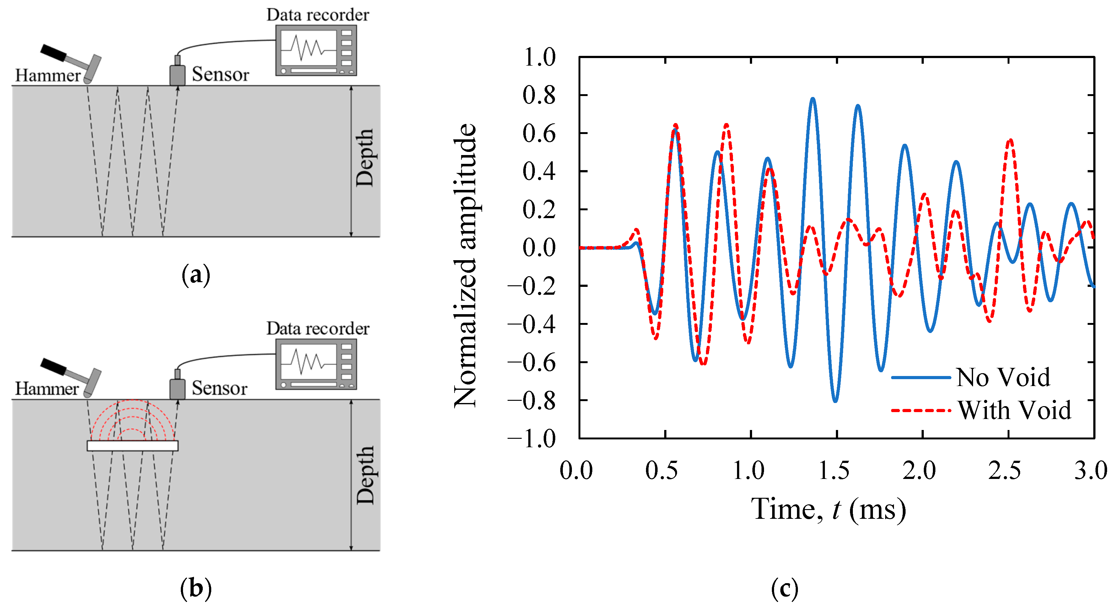
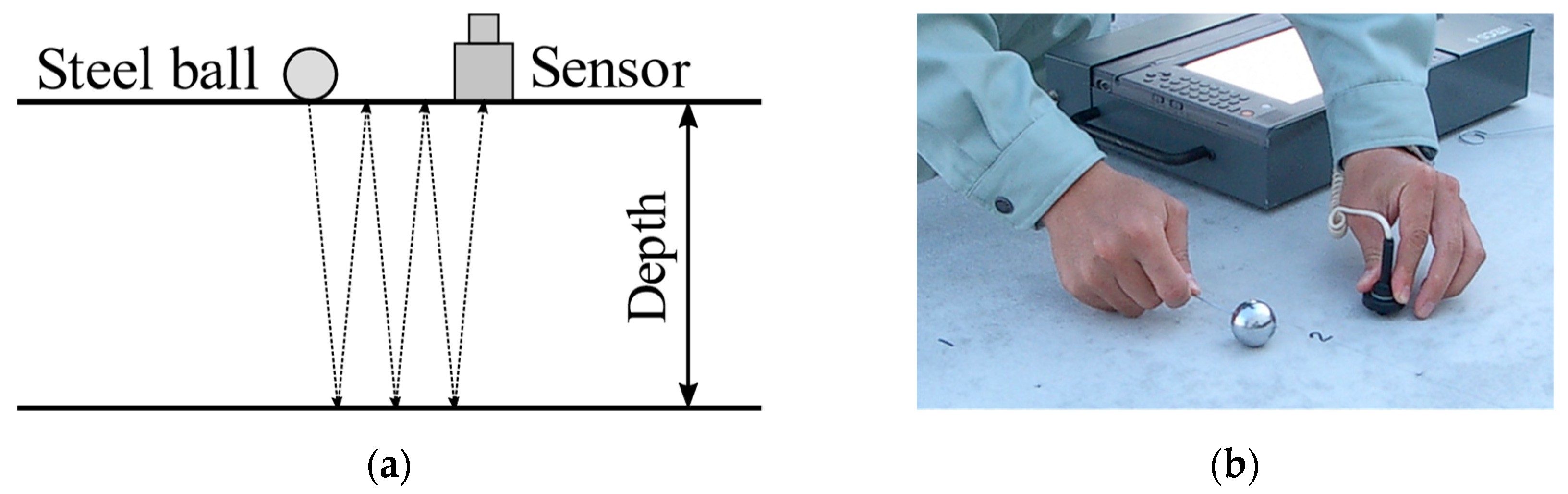
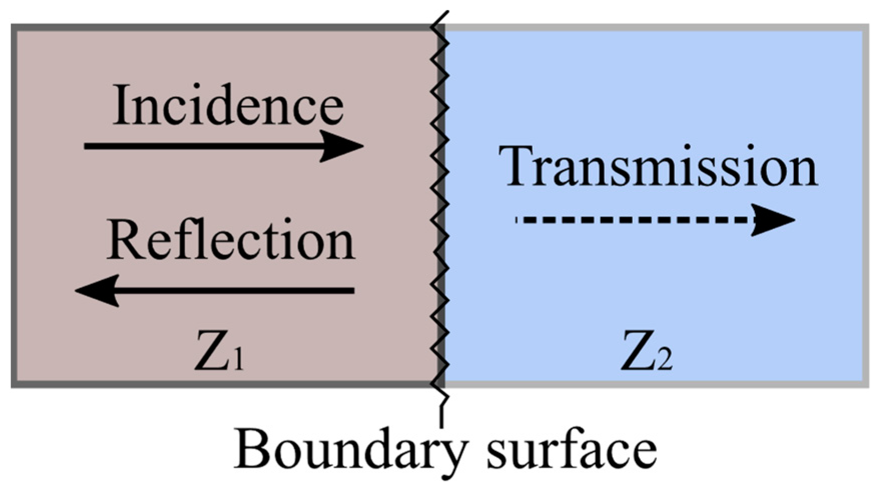
1.2. Impact Elastic Wave Method (IEW)

Figure 1a,b show the measurement schematic of the IEW method. The simplest way to measure IEW is to use a steel ball for the excitation. Figure 1b shows the photo of the excitation; the steel ball is attached to a handle, and it is used like swinging a hammer. The elastic wave is emitted by hitting the surface of the structure with the steel ball, and the response is measured on the surface in the vicinity of the hitting point. From the response of the surface, it is possible to evaluate the thickness of the structure and the presence of internal defects on the plate-like structures [4,5,6,7,8,9,10,11,12,13,14,15,16,17,18,19,20,21]. In addition, if excitation is given by the generally used steel ball size, the input frequency range is about 2 kHz to 20 kHz, which is lower than that of ultrasonic waves; input wavelength is long and the attenuation is small as a consequence. Furthermore, since a relatively low frequency band is used for the input, the effect of elastic waves due to dispersibility is very small [27]. This makes it suitable for the NDT of concrete structures with large thickness and composite materials.

The elastic wave is repeatedly reflected on boundary surfaces of different acoustic impedances [4,7,28,29]. The acoustic impedance is expressed as the product of the density and the elastic wave velocity in the medium, as shown in Equation (1):

$$Z=\rho V,$$

(1)

where Z is the acoustic impedance, ρ is the density of the medium and V is the elastic wave velocity of the medium. The reflectance of the elastic wave varies with the ratio of the acoustic impedance, which is calculated by Equation (2):

$${\gamma }_p=\frac{Z_2-Z_1}{Z_2{+Z}_1},$$

(2)

where γ_p is the reflectance, Z₁ (Z₁ = ρ₁V₁) is the acoustic impedance of the medium 1, and Z₂ (Z₂ = ρ₂V₂) is the acoustic impedance of the medium 2. Considering a model with a boundary surface as shown in Figure 2, if it is assumed that medium 1 is concrete and medium 2 is air and assuming the general physical properties are described as shown in

Table 1. Medium conditions.

Medium	ρ (kg/m3)	V (m/s)	Z (kg/s·m2)
1: Concrete	2400	4000	9.60 × 107
2: Air	1.29	332	4.28 × 103

, the calculated γ_p is about 1.0 from Equation (2), and it shows that the reflection is almost 100%. From such basic properties of the elastic waves, the thickness of a plate can be evaluated by using the characteristic of the elastic wave reflected repeatedly between the measuring and reflecting surfaces.

Figure 3a,b show an example of a schematic elastic wave path and its response waveform. The input elastic wave is reflected between the measuring surface and the reflecting surface. The natural frequency of the primary vibration mode by the multitude reflection of the elastic wave in the thickness direction is obtained from the round-trip distance and the primary elastic wave velocity of the thickness direction as follows:

$$F_0=\frac{V_P}{{2D}_0},$$

(3)

where F₀ is the natural frequency of the primary vibration mode, V_P is the primary elastic wave velocity in the thickness direction and is the phase velocity and D₀ is the thickness. Conversely, the thickness is shown as Equation (4) on the basis of Equation (3):

$$D_0=\frac{V_P}{{2F}_0}.$$

(4)

In practice, a technique to evaluate the thickness of concrete structures from the dominant frequency obtained by Fast Fourier Transform (FFT) of the measured wave and primary elastic wave velocity is established [4]. In addition, Sansalone et al. recommend that the V_P used in the calculation is corrected according to the shape of the target. In the case of a plate, the correction factor β (β = V_PP/V_P = 0.96) is used. This correction factor β varies depending on the cross-sectional shape of the measurement target [4].

This principle is also used in the techniques to evaluate the existence of internal defects. This utilizes the frequency change caused by the reflected wave from the boundary surface by defect and the apparent change in propagation distance bypassing the defect. Figure 4 shows a schematic of the propagation path of elastic waves around the internal void. Since elastic waves are reflected at the boundary of different acoustic impedance, the voids produce reflected waves as well. In addition, there are reflected waves that bypass the void and return from the bottom surface. The observed dominant frequency changes, due to the reflected waveform, the void and propagation path because of the influence of internal voids, and the evaluation of the internal defects is conducted by using the change of the dominant frequency [4,5,6,7,8,9,10]. However, there are difficulties to apply the technique to the evaluation if the size of the defect is small or the location is deep in the thickness direction [8,21].

Furthermore, in the case of a column member having a rectangular cross-section or beam member having a complicated cross-section as shown in Figure 5a,b, the propagation path is complicated on the cross-section that is orthogonal to the measuring surface and the reflecting surface. As a result, the multiple peak frequencies are observed and it makes it difficult to detect the frequencies that reveal the thickness [22,23,24,25]. For this reason, “ASTM-C1383-04” defined the configuration of the structure as a structure or portion of a structure in which the lateral dimensions are at least six times the thickness [26]. Therefore, the principle of thickness measurement cannot be applied to structures having these shapes. In other words, it is impossible to evaluate the defects by frequency as well. For overcoming difficulty, a new index that indicates the existence of the defects properly regardless of the shape of the structures has been demanded.

2. Difference Value Analysis (DVA)

2.1. Difference Value

The conventional technique can be applied only to the evaluation of plate-like structures. In contrast, DVA can be applied to the evaluation regardless of the shape of the structures. In particular, in the case of a structure constructed using commercialized concrete members, especially, DVA is a suitable index for the evaluation since it is possible to measure the response waveform in sound conditions. The response waveform in sound condition can be used for the evaluation of the other structures using the same product since it is considered that the product has the same response waveform in sound condition. This method uses the Difference value calculated based on the response waveforms of a structure in sound and damaged conditions in the time domain as the index value. Figure 6 shows a conceptual diagram of DVA. The difference of the models is only the existence of the void as shown in Figure 6a,b. Approximated propagation paths of the model are illustrated in Figure 6a,b as well, and Figure 6c shows the examples of response waveforms. The difference value is calculated as Equation (5), and the location and size of internal defects are evaluated on the basis of the difference value.

$$D_V=\frac{1}{N}{\displaystyle \sum }_{i=1}^N{{(f}_i-\stackrel{\prime }{f_i})}^2,$$

(5)

where D_V is the difference value, f_i is the amplitude of the response waveform at time step i without the void, $\stackrel{\prime }{f_i}$ is the amplitude of the response waveform at time step i with the void, and N is the number of data that are used for the calculation of the difference value. DVA evaluates the soundness in the thickness direction, mainly in the range between the input point and the measurement point. Therefore, N is determined to cover the time in which the reflected elastic wave in the thickness direction returns to the measurement point. The measurement time t required for this response is determined by Equation (6):

$$T=\frac{{2D}_C}{{\beta V}_P},$$

(6)

where D_C is the propagation distance in the thickness direction of the concrete structures, β is the correction factor and V_P is the primary elastic wave velocity. This correction factor β varies depending on the cross-sectional shape of the measurement target. Therefore, the minimum number of data required for calculation is determined by Equation (7) from the measurement time and sampling interval:

$$N_{\mathit{min}}=\frac{t}{\Delta t},$$

(7)

where N_min is the minimum number of data required for calculation and ∆t is the sampling interval.

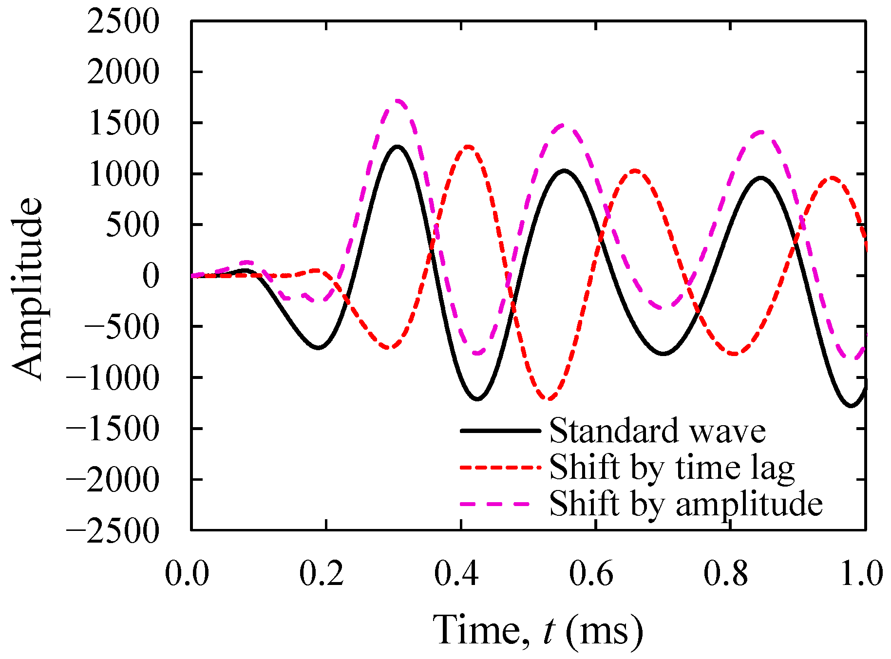
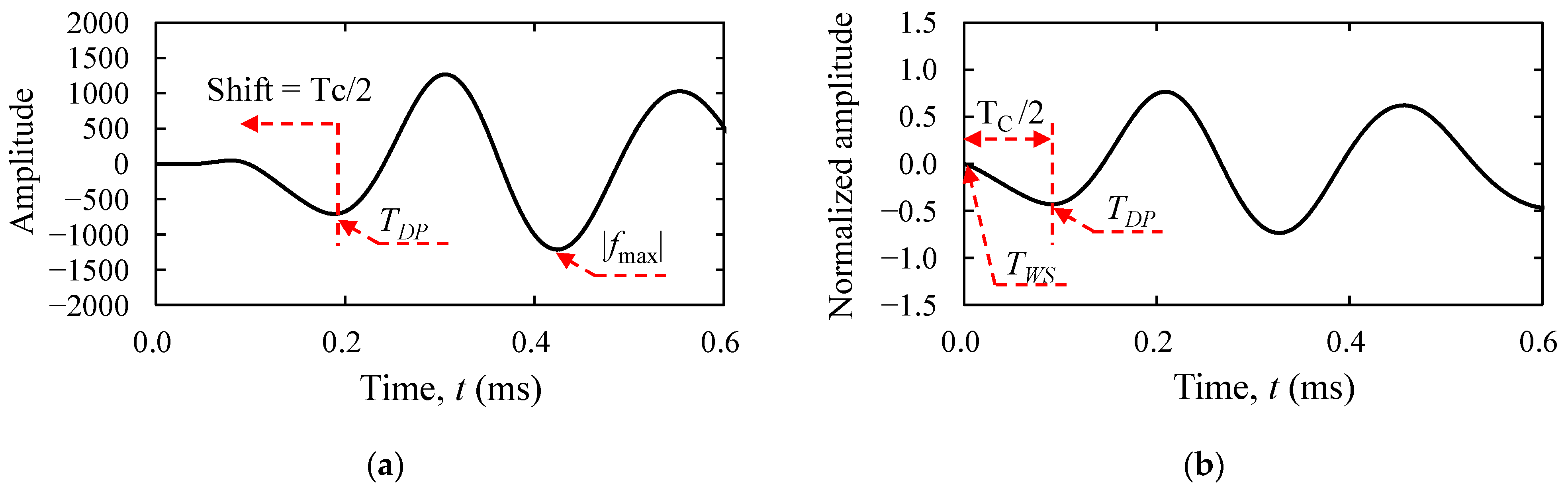
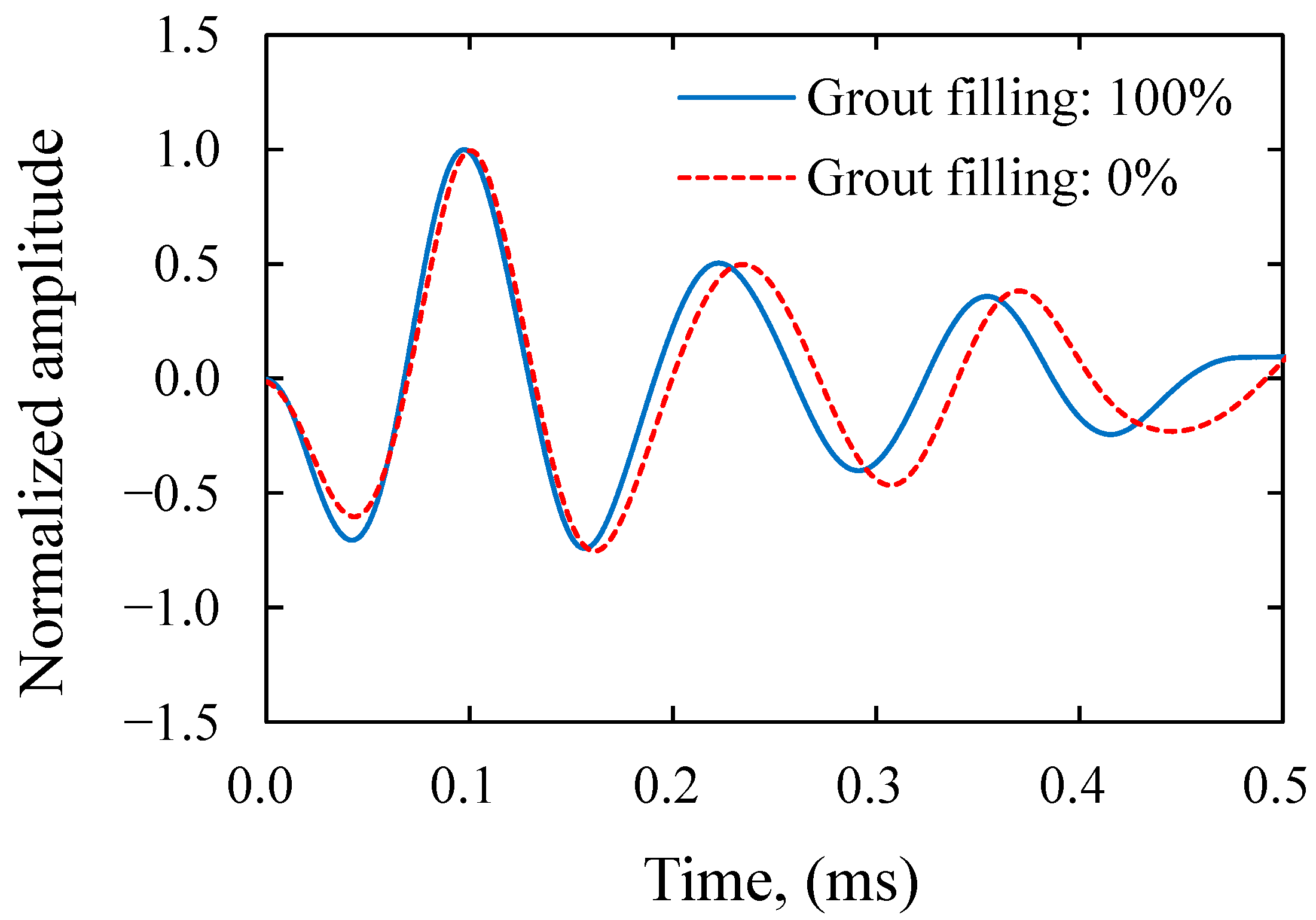
2.2. Normalization of Measured Waveform

Figure 7 shows an example of the variation of the response waveform that is measured at the same point. Since the input for IEW uses the artificial excitation with the steel ball, measurement errors occur due to the difference of the input energy and small deviations of the input point. This input method is also used for the measurements in this study. For this reason, the amplitude of the response waveform changes because the input energy slightly varies at each excitation. Due to the nature of the excitation method, it is difficult to precisely control the input energy. In addition, the time from the start of the recording to the arrival of the elastic wave generally varies in each measurement. The recording normally starts if the amplitude exceeds a threshold. In the case of measurement using a steel ball, recording starts when the elastic wave reaches the receiving point, and it is impossible to observe the time of the excitation. Therefore, DVA mainly evaluates internal defects using the change of the shape of the time history after the arrival of the elastic wave, and the adjustment of the initial time is conducted in DVA. These errors have a significant impact on the difference values, and it is necessary to normalize the amplitude of the measurement waveform and perform time correction. Hence, with the objective of reducing these sources of error, this study uses the following method for amplitude normalization and compensate for the time. For this reason, the difference value D_V used in this study is a dimensionless quantity.

In this study, the amplitude of the response waveform is normalized by the absolute value of the maximum amplitude as following Equation (8):

$$f_{\mathit{ni}}=\frac{f_i}{\left| f_{\mathit{max}} \right|},$$

(8)

where |f_max|is the maximum amplitude of f_i, f_i is the ith component of the time history of the amplitude and f_ni is the normalized amplitude of the time history. Figure 8a,b show an example of waveform normalization. The time shift is corrected by taking the first downward peak as the reference time and subtracting half of the contact time between the concrete and the steel ball as following Equation (9):

$$T_{\mathit{WS}}{=T}_{\mathit{DP}}-\frac{T_C}{2},$$

(9)

where T_WS is the wave start time after correction, T_WD is the downward peak time and T_C is the contact time of the steel ball. The contact time of the steel ball is calculated from Equation (10):

$$T_C=0{.0043d}_s,$$

(10)

which is a numerical solution of the contact time with the steel ball diameter d_s based on the theory and physical behavior of colliding solids proposed by Sansalone et al. [4,30]. The contact time T_C used in this study are all calculated by Equation (10).

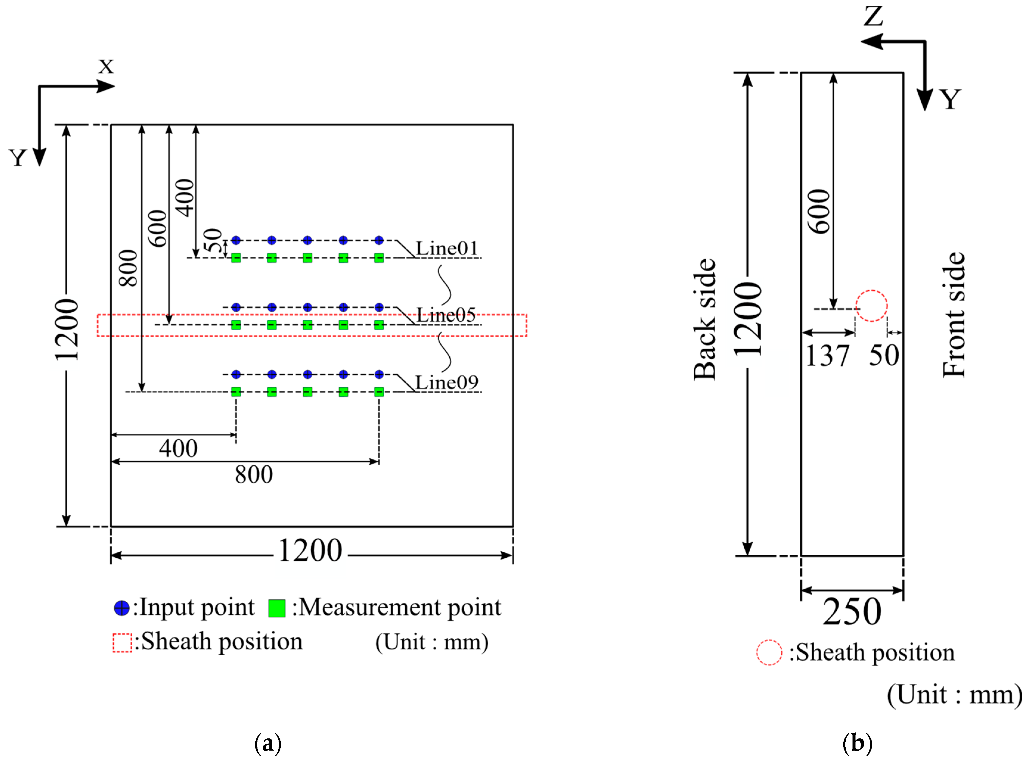
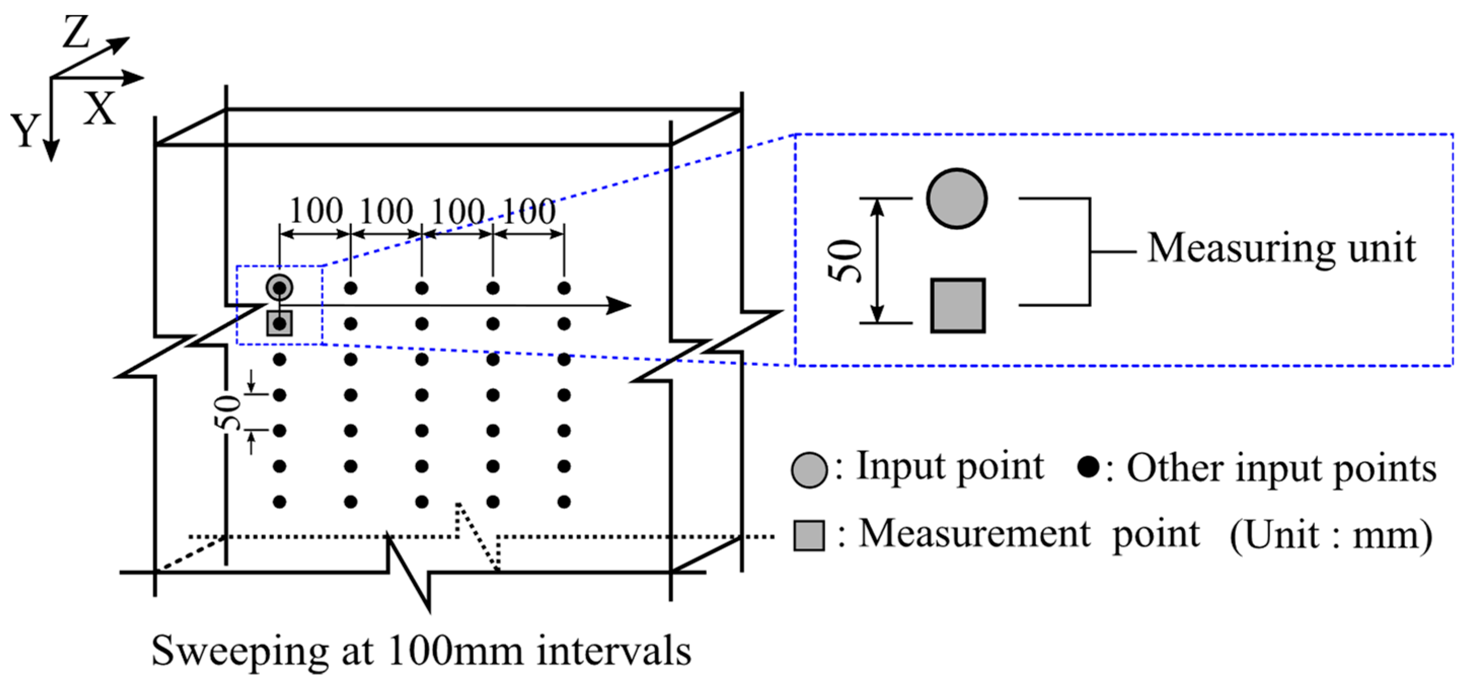
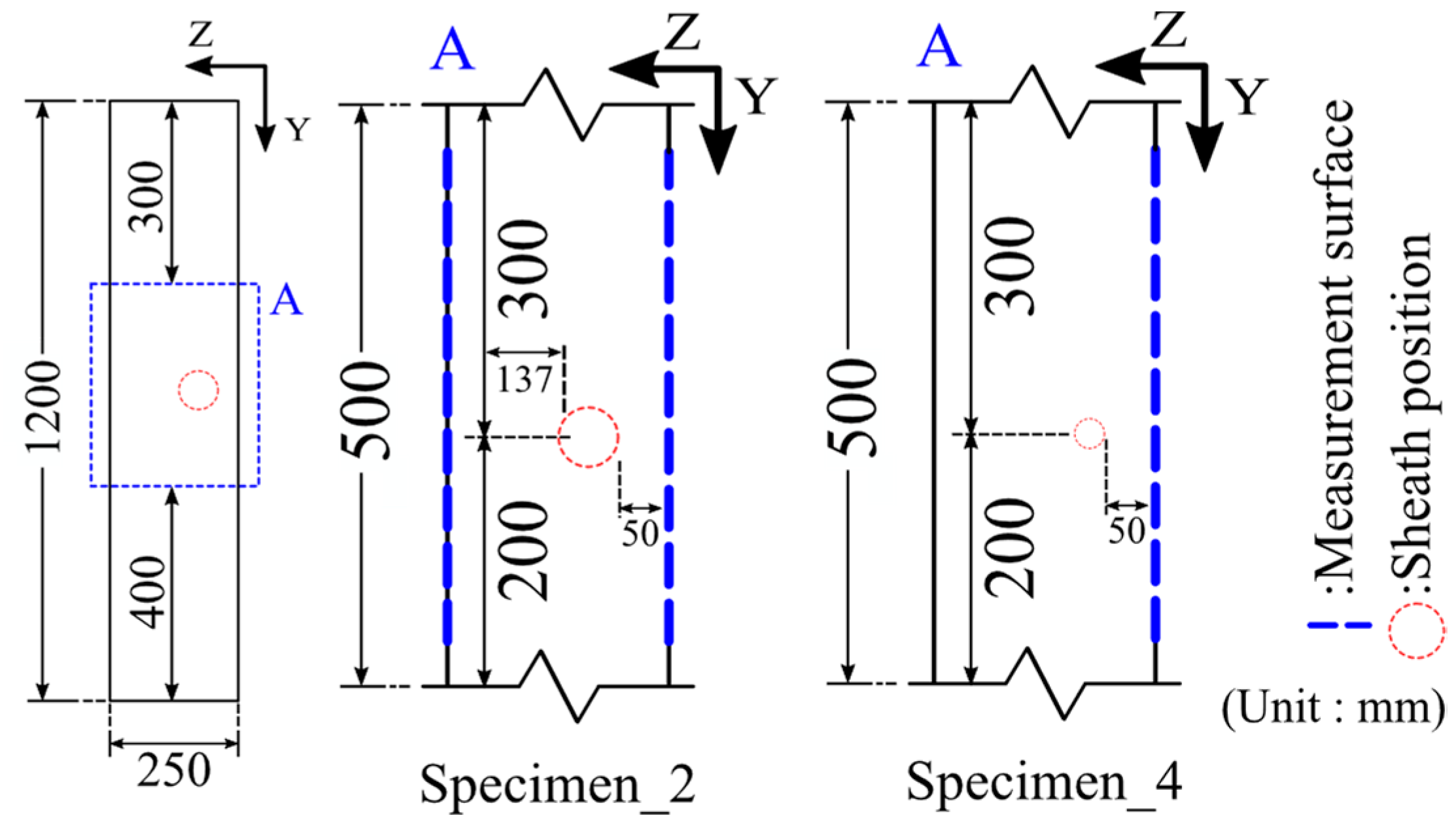
3. Experiment Conditions

In this study, model tests are performed for the validation of DVA with four concrete specimens in which an unfilled sheath is embedded. The specimen is made of concrete with the same mixing conditions using portland cement, and each specimen has the same configuration as illustrated in Figure 9a,b. A spiral sheath of 1300 mm in length is buried at 600 mm in the Y coordinate system and 50 mm in the Z coordinate system in the specimens, as shown in Figure 9. Figure 10a,b show a photograph of the specimen_1. In this experiment, four specimens are prepared with two grout filling patterns of 100% and 0% for each sheath diameter. The sheaths adopted are 63 mm and 33 mm in diameter.

Table 2. Sheath conditions.

Specimen_No.	Sheath Size: φS	Filling Ratio
Specimen_1	63 mm	100%
Specimen_2		0%
Specimen_3	33 mm	100%
Specimen_4		0%

shows the conditions of the sheaths. It is assuming that grout with 100% filling ratio simulates sound condition and the grout with 0% filling ratio simulates unsound condition. Difference value is calculated by using the response waveforms of the same sheath with different filling ratio and evaluate the unfilled sheath from the distribution of the calculated difference value. In addition, the influence of sheaths of different diameters is examined by comparing the difference values that are calculated by using the response waveforms of the different sheath and filling ratio.

Figure 11 show the schematic diagram of the structure and sweep direction of the input and measurement points. As shown in Figure 11, the distance between the input point and the measurement point is fixed at 50 mm, and the measurement is performed for each measurement point. Moreover, this measuring unit advances in the X-axis direction at a 100 mm interval and if the measurement is completed on the line, it is moved in the Y-axis direction at 50 mm intervals for further measurement to be performed. Thus, measurement and movement are repeated, and the measurement is performed at the condition of the coordinate positions of the input points in

Table 3. Location of the input points.

Line_No.		X (mm)	Input Point_No, (IP_No)
	Y (mm)		400	500	600	700	800
Line_01	350		IP_01	IP_02	IP_03	IP_04	IP_05
Line_02	400		IP_06	IP_07	IP_08	IP_09	IP_10
Line_03	450		IP_11	IP_12	IP_13	IP_14	IP_15
Line_04	500		IP_16	IP_17	IP_18	IP_19	IP_20
Line_05	550		IP_21	IP_22	IP_23	IP_24	IP_25
Line_06	600		IP_26	IP_27	IP_28	IP_29	IP_30
Line_07	650		IP_31	IP_32	IP_33	IP_34	IP_35
Line_08	700		IP_36	IP_37	IP_38	IP_39	IP_40
Line_09	750		IP_41	IP_42	IP_43	IP_44	IP_45

. The total number of measurement points is 45.

The receiving sensor is a high sensitivity acceleration sensor, and accelerometers are installed in the Z-axis direction to the X–Y plane, and impacts are made in the Z-axis direction. In this experiment, 5 measurement waveforms are recorded at the same measurement point, and the average waveform of the normalized waveforms is created, and the Difference value is calculated by using the averaged waveform. A comparative example of the waveform after all of the processing is shown in Figure 12.

In Specimens_1 and 2, the same measuring point is set on the backside. This changes the sheath from the measurement surface. The depth is as shown in Figure 9b. Comparing these results, the influence of the depth of the sheath on the difference value is investigated.

Table 4. Summarizes the sheath size and depth for all measurements.

Case _No	Sheath Size: φS	Depth
Case_1	63 mm	50 mm
Case_2	63 mm	137 mm
Case_3	33 mm	50 mm

summarizes the sheath size and depth for all measurements.

DVA measurement conditions are determined on the basis of thickness measurement by IEW. Therefore, it is possible to evaluate by using DVA with the same measurement waves for IEW. Thus, in this study, the results of DVA and IEW are compared. Since IEW estimates the target thickness based on the dominant frequency of multiple reflections of elastic waves between the measurement and reflection surfaces, the measurement conditions should be set appropriately so that the multiple reflections are sufficiently formed.

Table 5. Measurement conditions.

Diameter of steel ball	dS	20 mm
Contact time	Tc	0.086 ms
Input frequency	Finp	11.6 kHz
Measurement time	t	2.00 ms
Sampling time	Δt	0.50 μs
Measurement data		4000
Acceleration sensor		100 mV/G

shows the measurement conditions in this experiment.

The input frequency is calculated from the contact time of the steel balls used in the experiment as in the following Equation:

$$F_{\mathit{inp}}=\frac{1}{T_c},$$

(11)

where F_inp is the input frequency and$T_c$ is the contact time, respectively. In addition, since 10% of the number of measurement data are used for pre-trigger, the number of valid data after normalization is about 3600.

The number of calculated data for DVA can be determined arbitrarily from the number of measured data. To calculate the difference value, the number of data have to cover the time in which the reflected wave returns to the measurement point. In this study, we set the measurement conditions to satisfy the conditions. On the other hand, it should be carefully considered to make the number of data large because the influence of internal defects at a long distance is taken into account consequently. Therefore, the number of data is changed while the calculation of the difference value and its influence is examined as well.

4. Results

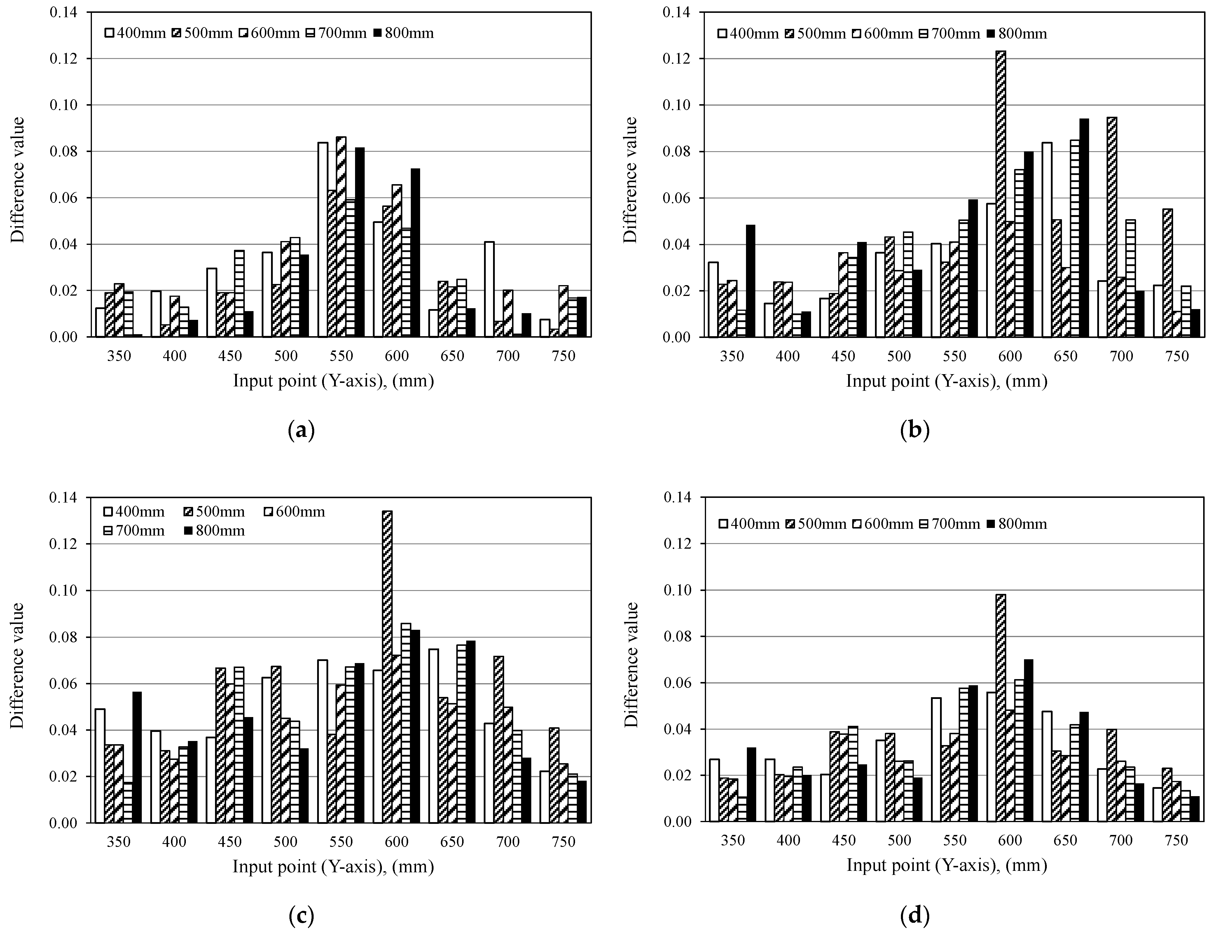
4.1. Influence of the Number of Data on the Calculation of Difference Value

4.1.1. Magnitude of Difference Value

Table 6. Propagation time and distance.

Number of Data: N	Propagation Time (μs)	Propagation Distance (mm)
100	50	200
250	125	500
500	250	1000
1000	500	2000
1500	750	3000
2000	1000	4000

shows a list of elastic wave propagation time and propagation distance that are obtained by assuming the longitudinal elastic wave velocity as 4000 m/s on various N. Figure 13, Figure 14 and Figure 15 show the resultant difference values of Case_1, Case_2, and Case_3 with N that is listed in Table 6, respectively. The horizontal axis shows the location of the input point on the Y-coordinate, the vertical axis shows the difference value, and the legend shows the location of the input point on the X-coordinate in these figures. In all the results, it is confirmed that the resultant difference value and its distribution change due to the change of N. It should be noted that the difference value with larger N decreases relatively. It is presumed that this is the effect of attenuation. The amplitude of the elastic wave attenuates due to the geometrical and material attenuation. Consequently, the influence of the input decays in the later part of the time history, and Difference value decreases if N is large because the influence of the input is averaged. Conversely, the difference value is larger if the N is adequately small since the influence of the input is emphasized. However, in all case, if comparing N = 100 and N = 250, the Difference value is smaller in N = 100 since the time width at N = 100 corresponds to 50 μs, which is shorter than the steel ball contact time of 86μs, and the reflected wave is not involved in the part of the time history. Finally, the change in the response waveform in the time domain is small because the measurement surfaces are the same condition. Consequently, it is considered that the Difference value is small, and it is revealed that the smaller Difference value is obtained if N is too small.

4.1.2. Distribution of the Difference Value

The distribution of the difference values in Figure 13a–f show that difference value increases relatively in the vicinity of the sheath position in all the results. In addition, in accordance with Figure 13a, it shows that the difference value increases at the sheath position even if the time in which the reflected wave returns from the reflecting surface is larger than the propagation time. In Case_1, 50 μs (N = 100) is greater than the arrival time of the reflected wave from the sheath of 25 μs. Thus, it is possible to detect the defect with smaller N if the depth of the defect is shallow. However, the location and size of the internal defects are generally unknown. Hence, if N is set not to cover the time in which the elastic waves return from the reflecting surface, it is not guaranteed that the soundness of thickness regions is evaluated correctly. Due to this, the tendency is different from Figure 13a in Figure 14a. In the case of Figure 14a, the arrival time of the reflected wave is 69 μs due to the change of sheath depth, which exceeds 50 μs of N = 100. As a result, the difference value does not increase at the sheath position because the reflected wave does not arrive until 50 μs from the sheath. Furthermore, Figure 15a shows that the increase of the difference value is not clearly observed although 50 μs satisfies the arrival condition of the reflected wave from the sheath. The input frequency of the IEW requires a sufficient wavelength to resonate the target. In this case, the elastic wave is not reflected sufficiently due to the wavelength, which is determined to give enough input wavelength for detecting the thickness. Therefore, the input frequency based on the thickness of the target might be inevitably low relative to the frequency to detect the defect location. In such input conditions, if the defect is small, it is difficult to establish a reflected wave between the defect and the measuring surface. For this reason, Sansalone et al. advocated that a high-frequency excitation is necessary to detect the small defects [4]. Because of these facts, it is concluded that it is difficult to capture the characteristic increase of the difference value with N = 100 in this case. Similarly, it is difficult to evaluate the sheath position from the distribution of the difference values if N is less than 1000 as shown in Figure 14b,c and Figure 15b,c. In contrast, the results for N = 1000 and above show the increase of the difference values at the sheath position. These results are obtained because of multiple reflections of the elastic wave between the measurement surface and the defect, and the increase of the different value is emphasized. In particular, the difference value clearly increases at the sheath location with N = 1000. As the introduced N should be adequately short, it is supposed that 1000 is the appropriate value of N to detect the sheath in this study. Hereafter, 1000 is adopted as N for further discussion.

The results indicate that N should be chosen to cover the time in which the multiple reflection is sufficiently formed between the sheath position subsequent. Based on the above discussion, it is revealed that DVA evaluates the position of the sheath correctly by choosing the appropriate N.

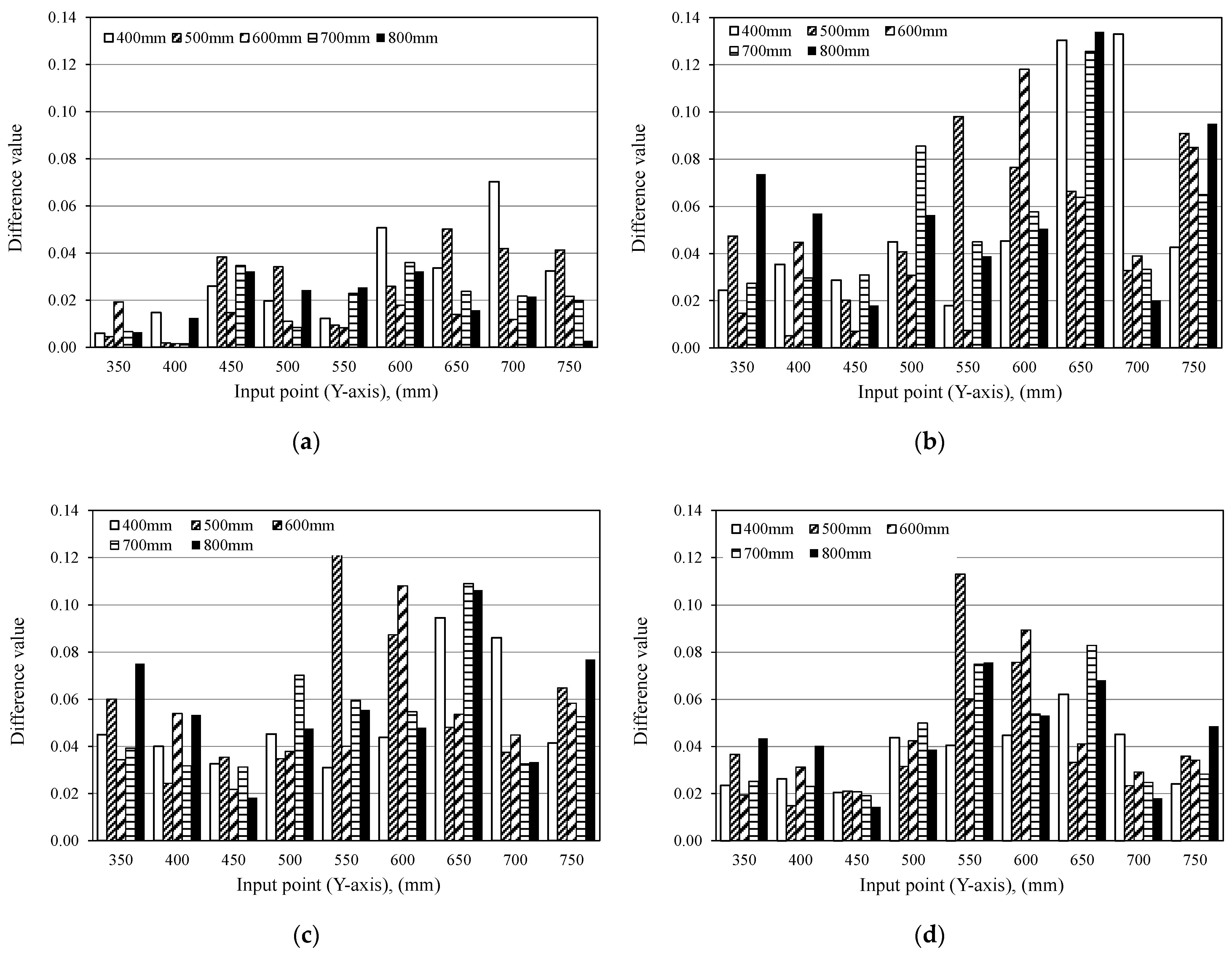
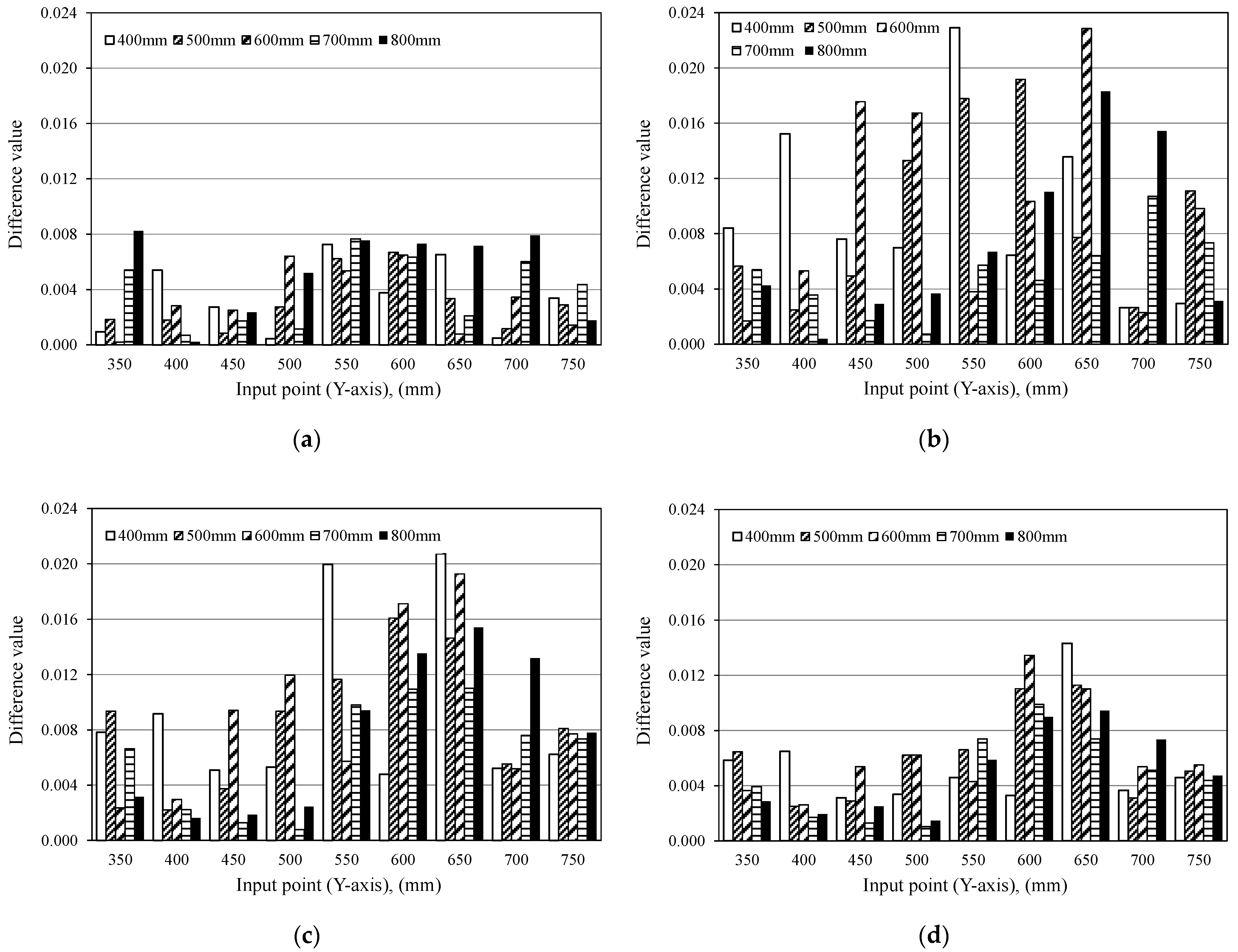
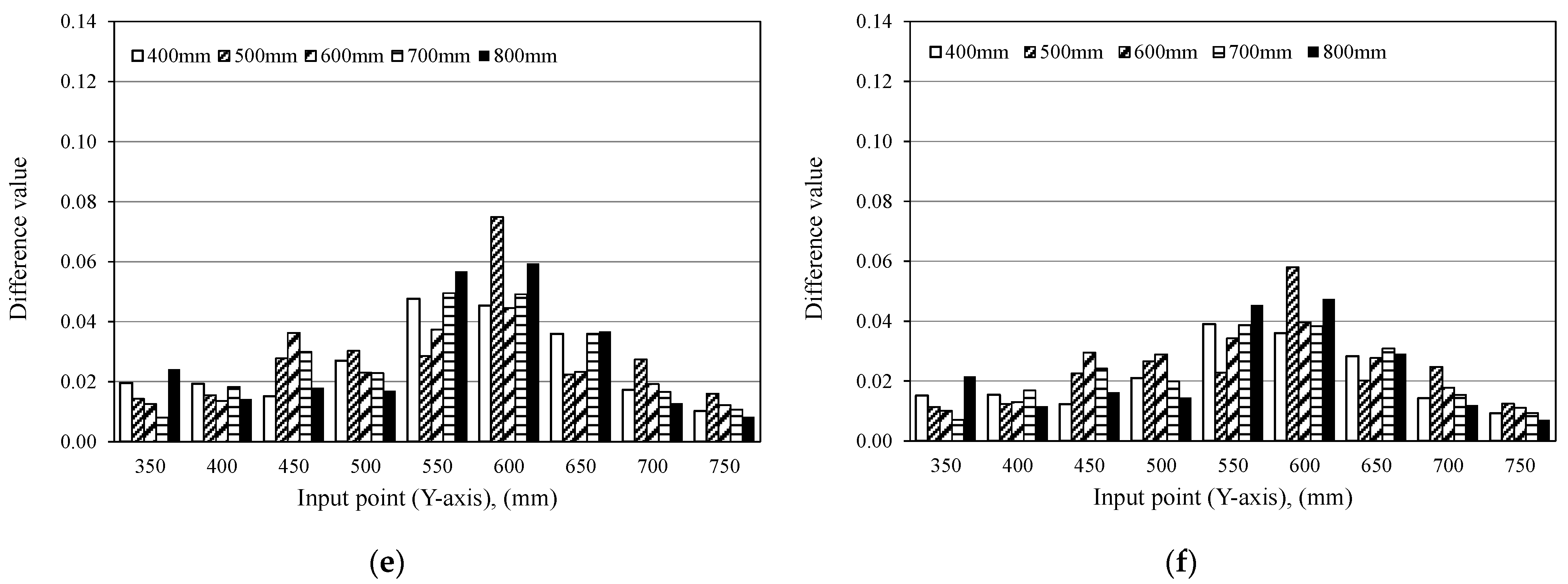
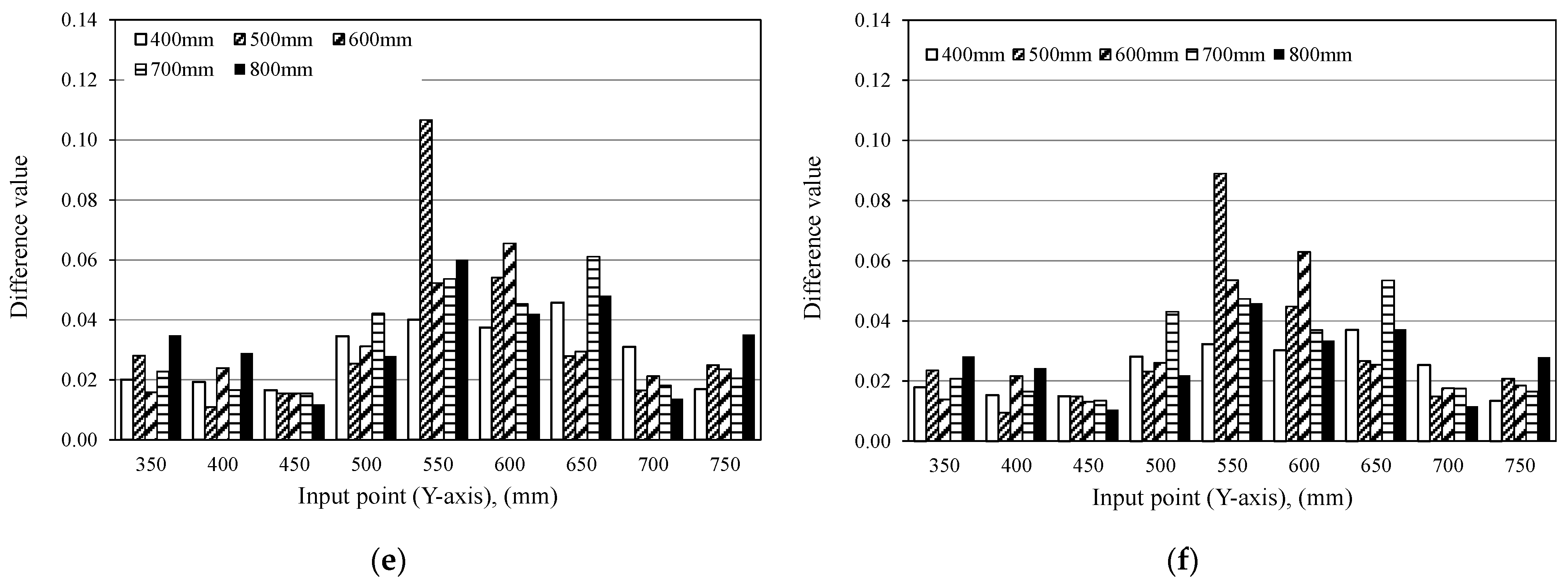
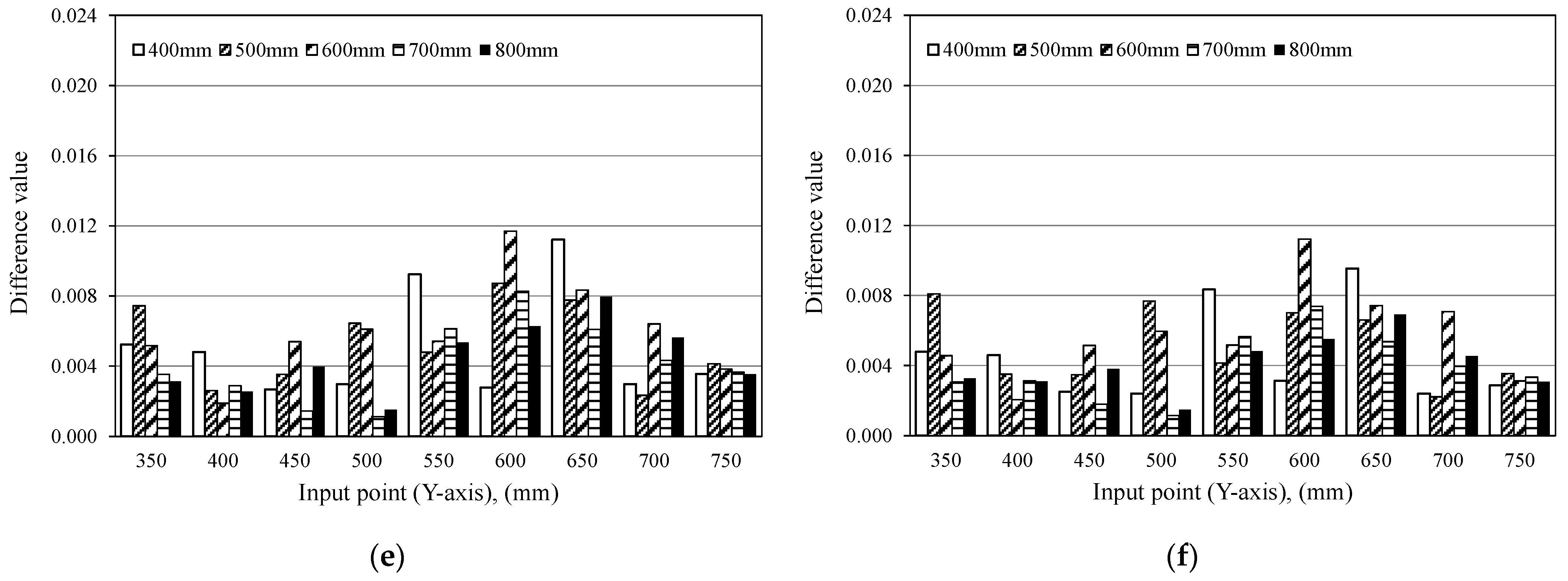
4.2. Distribution and Magnitude of Difference Values

Figure 16 shows a cross-section view of the specimen and configuration around the sheath of specimen_2 and specimen_4. Figure 17a,b show the comparison of the distribution of the difference values of specimen_2 and specimen_4 to consider the influence of the depth and diameter of the sheath. The X-coordinate of the input point for this result is 800 mm and N is 1000, respectively. In Figure 17a, the horizontal axis shows the Difference value, and the vertical axis shows the input point on the Y-coordinate, and the legend shows the depth. According to Figure 17a, the difference value increases between 550 mm to 650 mm in the coordinate of the input point, and the maximum Difference value is found at the 600 mm of the sheath position if the depth is 50 mm. However, if the depth is 137 mm, the Difference value increases between 500 mm and 700 mm. Compared to the depth of 50 mm, the range is enlarged 100 mm, and it demonstrates that the effect of the sheath is expanded.

Elastic waves three-dimensionally propagate in the specimen, and it spreads concentrically [7,8,9,10,11,12]. Thus, the propagation area of elastic waves increases with time. Because of this, if the location of the sheath is deep, the reflected waves from the sheath are expected to reach more extensive area. Figure 18a,b briefly illustrate the propagation and reflection of the elastic waves in a specimen with a void. In the case of Figure 18a, the propagation area is narrow because the distance between the measurement surface and the void is short. In contrast, in the case of Figure 18b, the distance between the measurement surface and sheath is longer, and the reflected wave from the sheath spreads wider. Finally, the response is affected widely on the measurement surface if the location of the void is deep. Therefore, if the location of the void is deeper, the Difference value increases over a wider area due to the influence on the reflected wave from the void. This suggests that DVA is capable to evaluate the depth of the void on the basis of the distribution of Difference value.

In Figure 17b, the horizontal axis shows the Difference value, the vertical axis shows the position of the input point on the Y-axis, and the legend shows the diameter of the sheath. According to Figure 17b, the Difference value increases between 550 mm and 750 mm and the maximum Difference value is observed at 650 mm in the case of φ_S = 33 mm. Similarly, a high Difference value is shown at 600 mm in the sheath position. These results indicate that DVA is capable to evaluate a small void as well. From this result, it is possible to be understand that the size of the void has a great influence on the Difference value.

Figure 19 shows the magnitude of the average Difference values of five measurement points on the input line (Line_06: Y = 600 mm) over the sheath. The horizontal axis shows the measurement case, and the vertical axis shows the Difference value. Comparing Case_1 and Case_2, the relative difference of the average error in the Difference value is 5.9% to the averaged Difference value of Case_1, and this implies that the sensitivity of the depth to Difference value is low. On the other hand, if Case_1 and Case_3 are compared, it shows that the relative average difference is 86.6%. This value is higher in comparison with the influence of depth and demonstrates the high impact of the size to Difference value.

From these results, it is suggested that the evaluation of the depth of the void based on the magnitude of the Difference value is difficult. However, since the range in which the Difference value increases becomes extensive if the location of the void is deep, it may be possible to evaluate the void depth from the distribution of the Difference value. In addition, the influence of the size of the void is bigger than the influence of the depth and it suggests that the size of the void is evaluated on the basis of the magnitude of the Difference value.

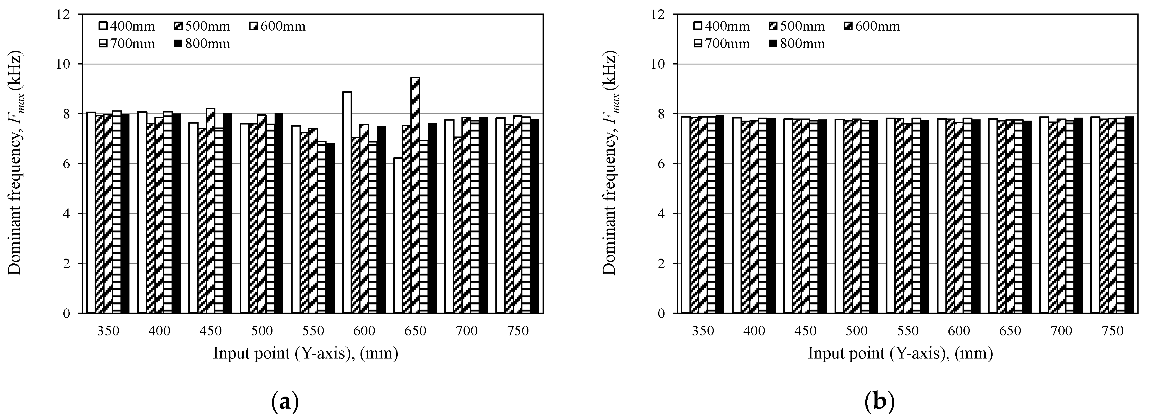
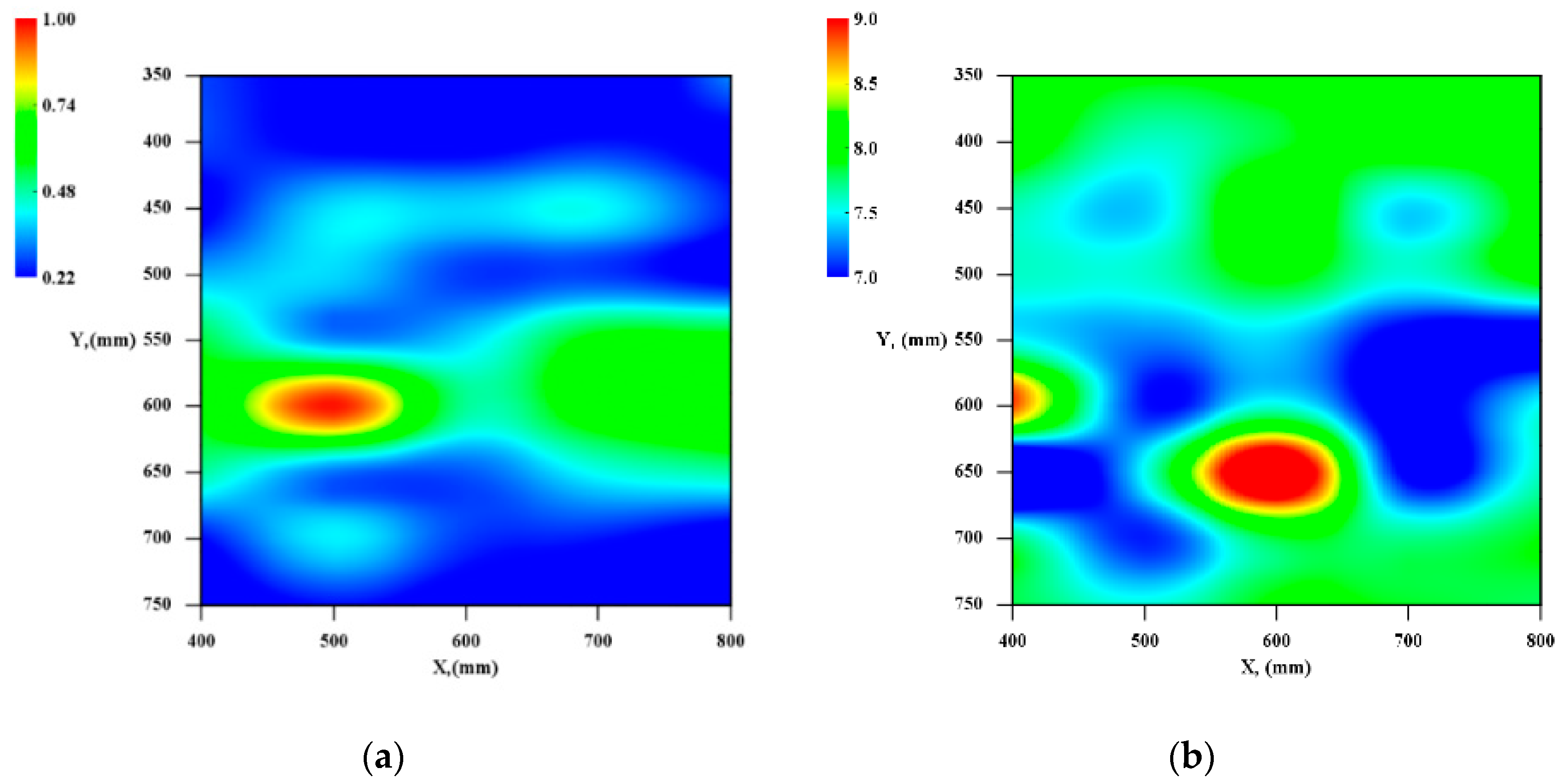
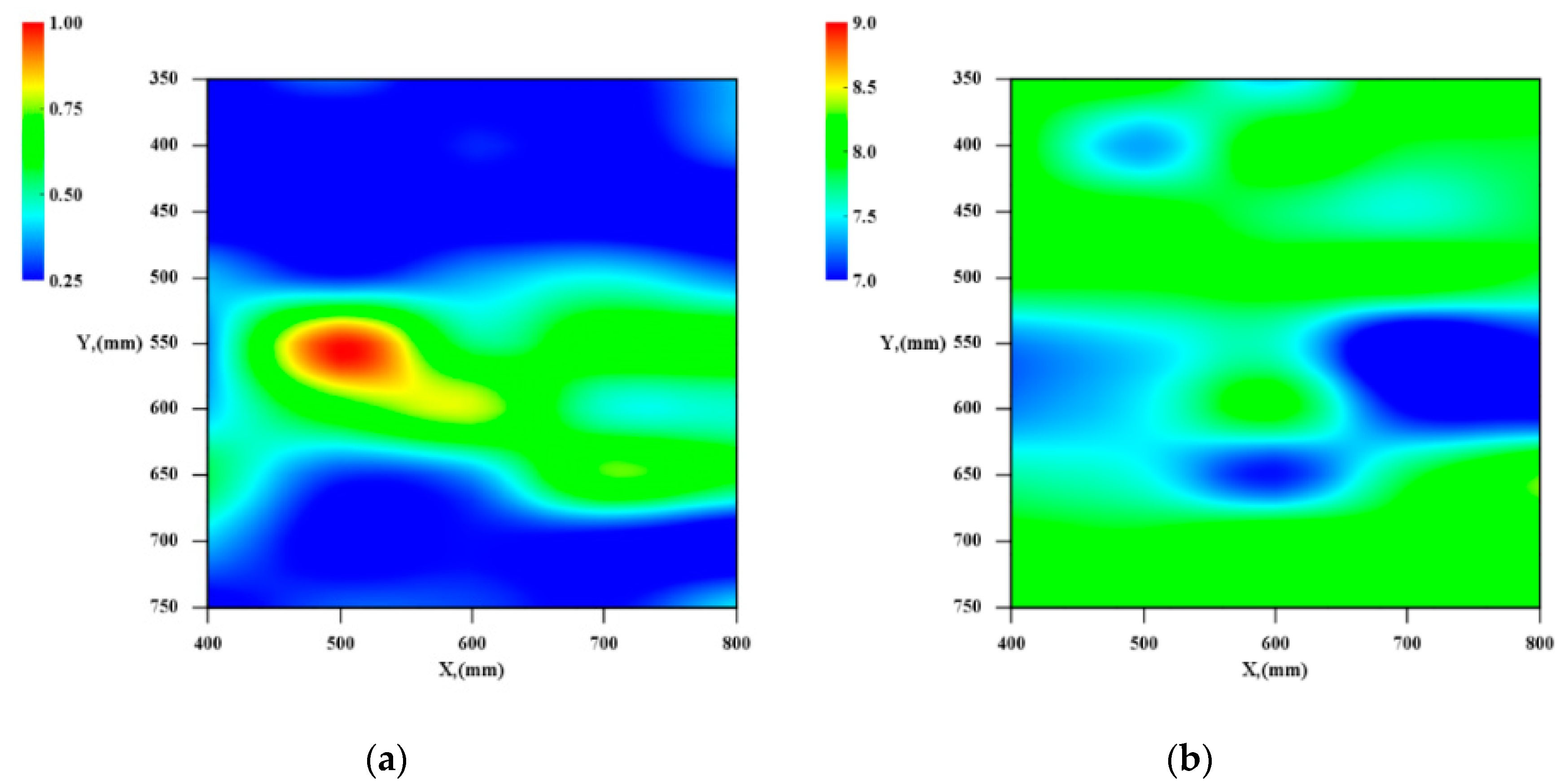
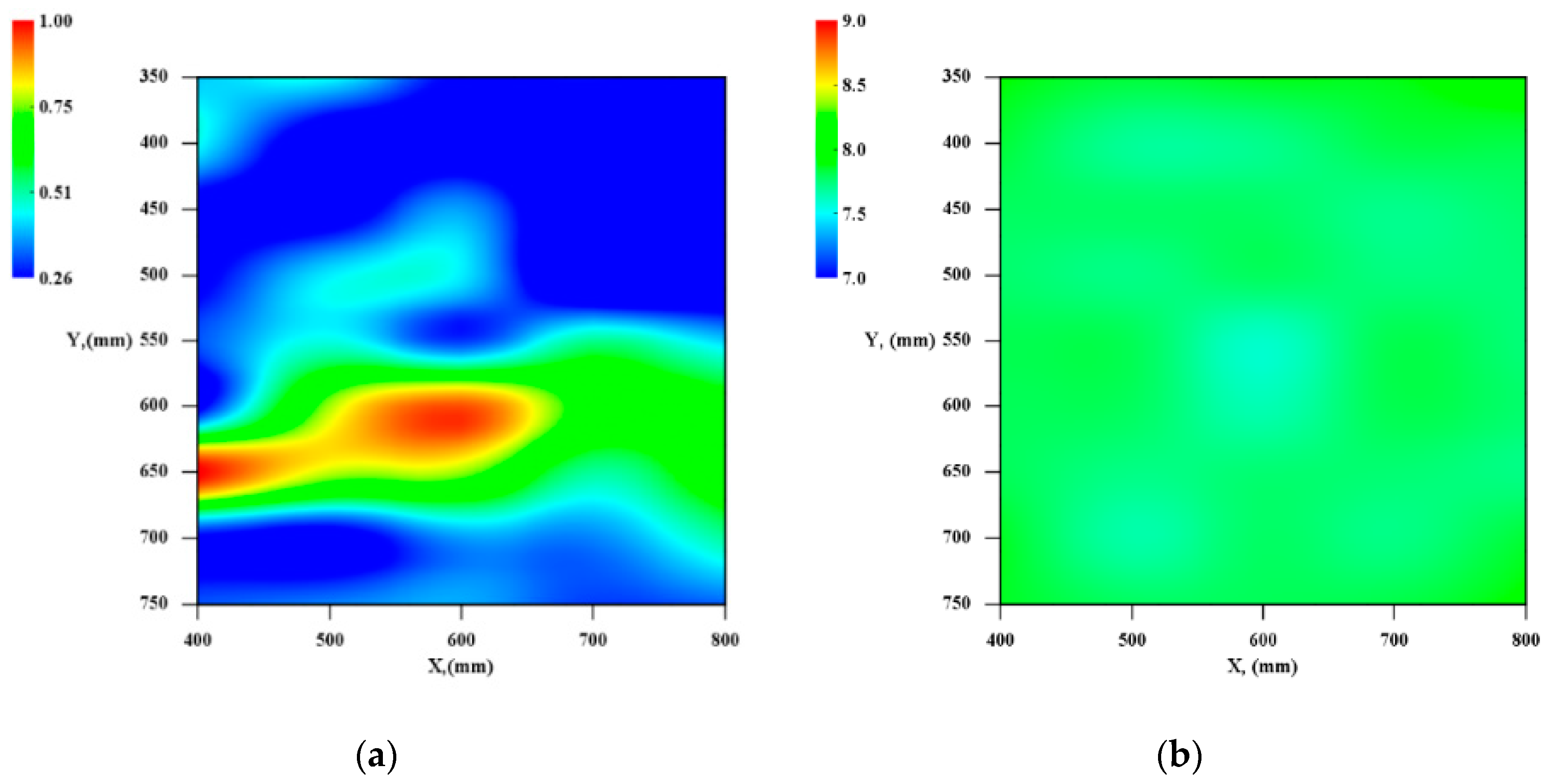
4.3. Comparison of DVA and Dominant Frequency Evaluation Results

The conventional IEW evaluates the thickness or existence of the void based on the natural frequency of the primary vibration mode in the thickness direction. In the evaluation, the peak frequency shifts higher due to multiple reflections between the measurement surface and the void, or it shifts lower because of a change in the apparent propagation distance. Therefore, the defects are evaluated by using the shift to the natural frequency. The natural frequency is calculated from the relationship between the primary elastic wave velocity and the thickness of the target on the basis of Equation (4). In the case of all specimens in this study, the thickness is given as 250 mm that is obtained as the distance between the measurement surface and reflection surface. Since the primary elastic wave velocity is not measured in these specimens, it is assumed as 4000 m/s, which is frequently used as a general concrete property. The natural frequency of the specimen is calculated from these constants as 8.0 kHz. In this study, this frequency is adopted as a reference value.

Figure 20a,b show the dominant frequencies of the response wave measured in this experiment. The horizontal axis shows the location of the input point on the Y-coordinate, the vertical axis shows the dominant frequency, and the legend shows the location of the input point on the X-coordinate. According to Figure 20a, it is found that the dominant frequency clearly changes if the input points exist between 550 mm and 650 mm. It is noted that this range indicates the vicinity of the sheath. In the other area, the dominant frequency is observed as 8.0 kHz that is obtained from the thickness of the specimen. On the other hand, in Figure 20b, 8.0 kHz is given as the dominant frequency in all results. Therefore, it is inferred that it is difficult to detect the diameter sheath of 33 mm on the basis of dominant frequency in this experimental condition.

Figure 21a,b, Figure 22a,b and Figure 23a,b illustrate the contours of the Difference value and dominant frequency that are calculated from the results of the experiments. The horizontal and vertical axes of the figure are the XY coordinates of input point on the measurement surface. The legend in (a) shows the Difference value normalized by the maximum Difference value of each experiment. In Figure 21a,b, both evaluation results show a change in the value around the sheath position. The similar tendency is observed in Figure 22a,b as well. These results demonstrate that both methods detect the sheath successfully. However, in Figure 23b, it is shown that the change of the dominant frequency is not detected around the sheath. In contrast, Figure 23a shows an increase in the Difference value in the vicinity of the sheath, and it suggests that DVA detects the relatively small defect that is not detected by the conventional method. Based on the discussion above, the experimental results so far show that DVA performs as well as the conventional evaluation methods. It is predicted that the problem would be overcome by changing the input frequency and the interval of the input and measurement points. However, it increases the measurement procedure and analysis time. In contrast, it is confirmed that DVA has the potential to evaluate the relatively small voids with a single measurement result.

5. Conclusions

This study, in order to overcome the difficulty of conventional internal defect evaluation, proposed a new evaluation method called DVA that uses Difference value as the evaluation index. The proposed method is validated experimentally by performing the model tests. The demonstrated results show that DVA detects the sheath as well as the conventional evaluation methods, and further, it suggests that DVA detects the relatively small defect that is not detected by the conventional method. The findings and conclusions of the research are summarized as follows:

• It is confirmed that the magnitude and distribution of Difference value depend on the number of data N. This arises from the influence of the input decays in the later part of the time history, and Difference value decreases if N is large because the influence of the input is averaged. Conversely, the Difference value is larger if the N is adequately small since the influence of the input is emphasized. On the other hand, if the number of data does not satisfy the contact time of the steel ball, the Difference value decreases because the reflected wave has no interference with the time history and the input condition and surface do not change. Further, if the number of data is not sufficient to cover the target thickness, of the defects depth and contact time, it is difficult to properly evaluate the internal defect. In addition, even if the thickness condition is complied with, the evaluation of internal defects becomes difficult because the difference value of the defects area is not characteristically increased with a small number of data. In contrast, as the number of data increases, the change of Difference value at the location of the defect is emphasized by the change of the reflected wave between the measurement surface and the defect and the change in the propagation path. From these results, it is revealed that DVA evaluates the position of the sheath correctly by choosing the appropriate N.
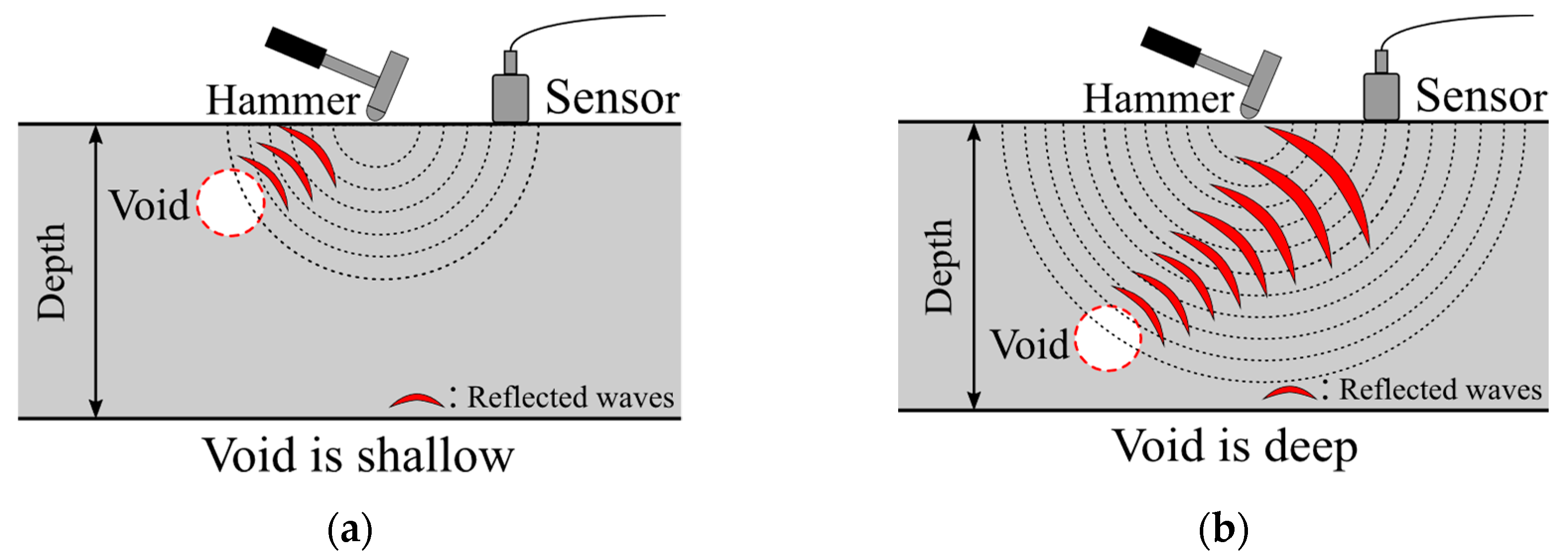
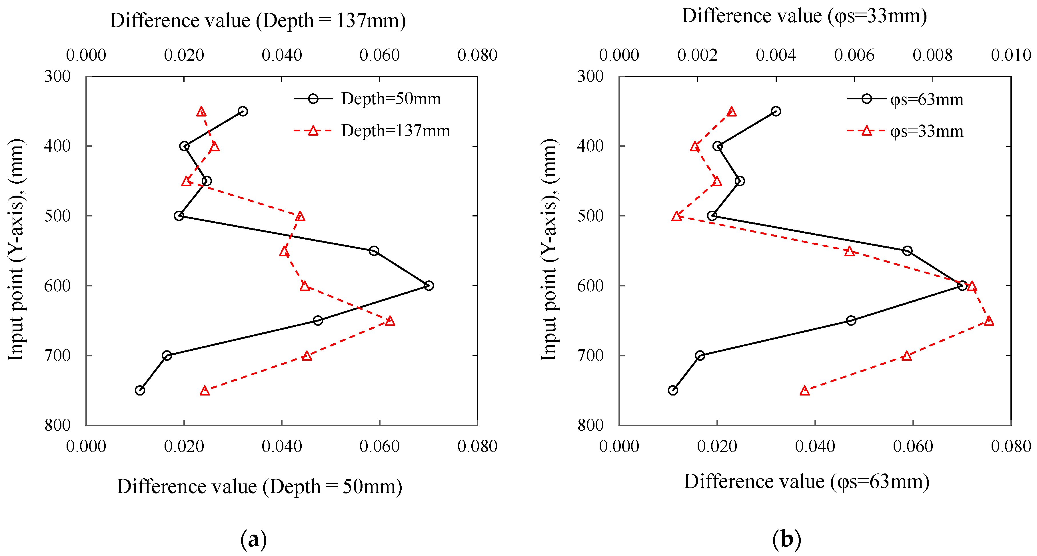
• The depth of the internal defect has the small influence for the magnitude of the difference value, and it is difficult to evaluate the depth of the defect of the same size from the magnitude of the difference value. However, it is confirmed that the difference value increases area if the defect is deep. This result suggests that the depth of the defect is possibly evaluated from the distribution of the difference values.
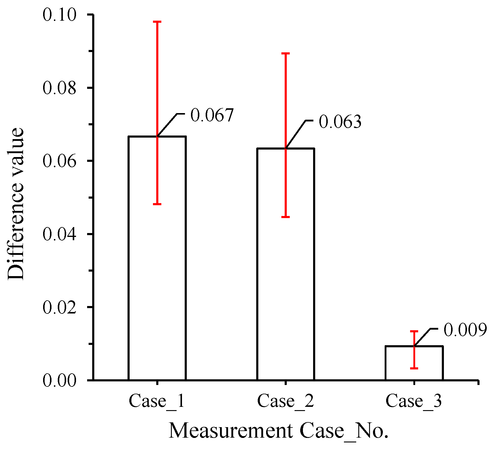
• It is confirmed that the size of the defect has a great influence of the difference value, and it is suggested that the size of the internal defect can be evaluated by difference values.
• Finally, comparing the evaluation results of the conventional method and DVA, it is found that DVA has the equivalent capability, and furthermore, it has the potential to evaluate relatively small defects that are not detected by the conventional method

References

1. Portland Cement Association. 2016 U.S. Cement Industry Annual Yearbook; Construction Facts, Industry Trends and Domestic & International Coverage: Old Orchard Road Skokie, IL, USA, 2016. [Google Scholar]
2. Omar, T.; Nehdi, M.L. Condition Assessment of Reinforced Concrete Bridges: Current Practice and Research Challenges. Infrastructures 2018, 3, 36. [Google Scholar] [CrossRef] [Green Version]
3. Kim, J.J.; Kim, A.-R.; Lee, S.-W. Artificial Neural Network-Based Automated Crack Detection and Analysis for the Inspection of Concrete Structures. Appl. Sci. 2020, 10, 8105. [Google Scholar] [CrossRef]
4. Sansalone, M.; Streett, W.B. Impact-Echo: Nondestructive Testing of Concrete and Masonry; Bullbrier Press: Ithaca, NY, USA, 1997. [Google Scholar]
5. Sansalone, M. Impact-Echo: The Complete Story. ACI J. 1997, 94, 777–786. [Google Scholar]
6. Sansalone, M.; Carino, N.J. Impact-Echo: A Method for Flaw Detection in Concrete Using Transient Stress Waves, NBSIR 86-3452. 1986. Available from NTIS, Springfield, VA, 22161, PB #87-104444/AS. Available online: https://www.rjlg.com/materials-insights/nondestructive-evaluation-nde-of-concrete-with-impact-echo/ (accessed on 5 May 2021).
7. Carino, N.J. Training: Often the Missing Link in Using NDT Methods. Constr. Build. Mater. 2013, 38, 1316–1329. [Google Scholar] [CrossRef]
8. Carino, N.J. The Impact-Echo Method: An Overview1. NIST 2001, 1–18. [Google Scholar] [CrossRef] [Green Version]
9. Carino, N.J. Impact Echo: The Fundamentals. In Proceedings of the International Symposium Non-Destructive Testing in Civil Engineering (NDT-CE), Berlin, Germany, 15–17 September 2015. [Google Scholar]
10. Carino, N.J.; Sansalone, M. Flaw Detection in Concrete Using the Impact-Echo Method. Bridge Eval. Repair Rehabil. 1990, 187, 101–118. [Google Scholar]
11. Jaeger, B.J.; Sansalone, M.J.; Poston, R.W. Detecting Voids in Grouted Tendon Ducts of Post-Tensioned Concrete Structures Using the Impact-Echo Method. ACI J. 1996, 93, 462–473. [Google Scholar]
12. Abraham, O.; Cote, P. Impact-echo thickness frequency profiles for detection of voids in tendon ducts. ACI J. 2002, 99, 239–247. [Google Scholar]
13. Zou, C.; Chen, Z.; Dong, P.; Chen, C.; Cheng, Y. Experimental and Numerical Studies on Nondestructive Evaluation of Grout Quality in Tendon Ducts Using Impact-Echo Method. J. Bridge Eng. 2014, 21, 04015040. [Google Scholar] [CrossRef]
14. Yoon, Y.-G.; Lee, J.-Y.; Choi, H.; Oh, T.-K. A Study on the Detection of Internal Defect Types for Duct Depth of Prestressed Concrete Structures Using Electromagnetic and Elastic Waves. Materials 2021, 14, 3931. [Google Scholar] [CrossRef]
15. Ohtsu, M.; Watanabe, T. Stack Imaging of Spectral Amplitudes based on Impact-Echo for Flaw Detection. NDT E Int. 2002, 35, 189–196. [Google Scholar] [CrossRef]
16. Muldoon, R.; Chalker, A.; Forde, M.C.; Ohtsu, M.; Kunisue, F. Identifying voids in plastic ducts in post-tensioning prestressed concrete members by resonant frequency of impact-echo, SIBIE and tomography. CBM 2007, 21, 527–537. [Google Scholar]
17. Hashimoto, K.; Shiotani, T.; Ohtsu, M. Application of Impact-Echo Method to 3D SIBIE Procedure for Damage Detection in Concrete. Appl. Sci. 2020, 10, 2729. [Google Scholar] [CrossRef] [Green Version]
18. Ma, M.; Cao, R.; Niu, C.; Zhang, H.; Liu, W. Influence of Soil Parameters on Detecting Voids behind a Tunnel Lining Using an Impact Echo Method. Appl. Sci. 2019, 9, 5403. [Google Scholar] [CrossRef] [Green Version]
19. Kentaro, Y.; Tomoaki, S.; Kunio, G. Detection of internal defects of concrete structures by analyzing wave speed scattering. S F R Proc. 2012, 14. [Google Scholar]
20. Shinya, U.; Oshiro, K.; Oshiki, I.; Satoshi, I.; Heung, L. A Study on Frequency Analysis Methods for Concrete Thickness Estimation by Impact Elastic-Wave Method. SCMT3 Proc. 2013, 3. [Google Scholar]
21. Abraham, O.; Léonard, C.; Côte, P.; Piwakowski, B. Time Frequency Analysis of Impact-Echo Signals: Numerical Modeling and Experimental Validation. ACI J. 2000, 97, 645–657. [Google Scholar]
22. Lin, Y.; Sansalone, M. Transient Response of Thick Circular and Square Bars Subjected to Transverse Elastic Impact. J. ASA 1992, 91, 885–893. [Google Scholar] [CrossRef]
23. Lin, Y.; Sansalone, M. Detecting Flaws in Concrete Beams and Columns Using the Impact-Echo Method. ACI J. 1992, 89, 394–405. [Google Scholar]
24. Popovics, S.J. Effect of Poisson’s Ratio on Impact-Echo Method Analysis. J. Eng. Mech. 1997, 123, 843–851. [Google Scholar] [CrossRef]
25. Hsiao, C.; Cheng, C.C.; Liou, T.; Juang, Y. Detecting flaws in concrete blocks using the impact-echo method. NDT E Int. 2008, 41, 98–107. [Google Scholar] [CrossRef]
26. ASTM C1383-04. Test Method for Measuring the P-Wave Speed and the Thickness of Concrete Plates Using the Impact-Echo Method; ASTM Standards: West Conshohocken, PA, USA, 2010. [Google Scholar]
27. Ospitia, N.; Aggelis, D.G.; Lefever, G. Sensor Size Effect on Rayleigh Wave Velocity on Cementitious Surfaces. Sensors 2021, 21, 6483. [Google Scholar] [CrossRef] [PubMed]
28. Krautkrämer, J.; Krautkrämer, H. Ultrasonic Testing of Materials, 4th ed.; Springer: New York, NY, USA, 1990; pp. 15–18. [Google Scholar]
29. Toshiro, K.; Shinya, U. Theory and practice of NDT of concrete: No.3 Theory and practice of elastic wave method (ultrasonic method/impact elastic wave method). J. JCI 2013, 51, 340–347. (In Japanese) [Google Scholar]
30. Goldsmith, W. Impact: The Theory and Physical Behavior of Colliding Solids; Edward Arnold Press, Ltd.: London, UK, 1965; pp. 24–50. [Google Scholar]
Figure 1. IEW method: (a) Schematic illustration of the IEW method; (b) Photograph of measurement status.
Applsci 11 11402 g001
Figure 2. Reflection and transmission of elastic waves.
Applsci 11 11402 g002
Figure 3. Schematic illustration of the IEW method: (a) Schematic wave path; (b) Example of waveform.
Applsci 11 11402 g003
Figure 4. Schematic of the propagation path and frequency of elastic waves in the internal void.
Applsci 11 11402 g004
Figure 5. Schematic of the propagation path of multiple reflection: (a) Rectangular cross-section; (b) Complex shaped beam.
Applsci 11 11402 g005
Figure 6. Concept of Difference value Analysis in Time Domain: (a) No void; (b) With void; (c) Example of response waveform comparison.
Applsci 11 11402 g006
Figure 7. Measurement waveform.
Applsci 11 11402 g007
Figure 8. Example of waveform normalization: (a) Before normalization; (b) After normalization.
Applsci 11 11402 g008
Figure 9. Schematic diagram of the specimen_1 and specimen_2: (a) Front side of specimen; (b) Cross-section view of configuration and the sheath.
Applsci 11 11402 g009
Figure 10. Photograph of the concrete specimen_1: (a) Front side of specimen; (b) Cross-section of specimen.
Applsci 11 11402 g010
Figure 11. Schematic diagram of the structure and sweep direction of the input and measurement points.
Applsci 11 11402 g011
Figure 12. Example of response waveform after normalization (Case_1: φS = 63 mm).
Applsci 11 11402 g012
Figure 13. DVA results for Case_1 (φS: 63 mm, Depth: 50 mm): (a) N = 100; (b) N = 250; (c) N = 500; (d) N = 1000; (e) N = 1500; (f) N = 2000.
Applsci 11 11402 g013aApplsci 11 11402 g013b
Figure 14. DVA results for Case_2 (φS: 63 mm, Depth: 137 mm): (a) N = 100; (b) N = 250; (c) N = 500; (d) N = 1000; (e) N = 1500; (f) N = 2000.
Applsci 11 11402 g014aApplsci 11 11402 g014b
Figure 15. DVA results for Case_3 (φS: 33 mm, Depth: 50 mm): (a) N = 100; (b) N = 250; (c) N = 500; (d) N = 1000; (e) N = 1500; (f) N = 2000.
Applsci 11 11402 g015aApplsci 11 11402 g015b
Figure 16. Cross-section view of specimen surfaces and configuration and the sheath.
Applsci 11 11402 g016
Figure 17. DVA results (X-axis of point = 800 mm): (a) Comparison by depth; (b) Comparison by sheath diameter.
Applsci 11 11402 g017
Figure 18. Schematic illustration of the propagation of the reflected waves due to change in void depth: (a) Shallow void; (b) Deep void.
Applsci 11 11402 g018
Figure 19. Comparison of average and error bars of Difference value on a sheath position (Line_06).
Applsci 11 11402 g019
Figure 20. Dominant frequencies: (a) Case_1: φS = 63 mm, Depth = 5 0 mm; (b) Case_3: φS = 33 mm, depth = 50 mm.
Applsci 11 11402 g020
Figure 21. Contours of the evaluation results for Case_1: (a) DVA; (b) Dominant frequency.
Applsci 11 11402 g021
Figure 22. Contours of the evaluation results for Case_2: (a) DVA; (b) Dominant frequency.
Applsci 11 11402 g022
Figure 23. Contours of the evaluation results for Case_3: (a) DVA; (b) Dominant frequency.
Applsci 11 11402 g023