Tri-Partition Alphabet-Based State Prediction for Multivariate Time-Series

Abstract

Recently, predicting multivariate time-series (MTS) has attracted much attention to obtain richer semantics with similar or better performances. In this paper, we propose a tri-partition alphabet-based state (tri-state) prediction method for symbolic MTSs. First, for each variable, the set of all symbols, i.e., alphabets, is divided into strong, medium, and weak using two user-specified thresholds. With the tri-partitioned alphabet, the tri-state takes the form of a matrix. One order contains the whole variables. The other is a feature vector that includes the most likely occurring strong, medium, and weak symbols. Second, a tri-partition strategy based on the deviation degree is proposed. We introduce the piecewise and symbolic aggregate approximation techniques to polymerize and discretize the original MTS. This way, the symbol is stronger and has a bigger deviation. Moreover, most popular numerical or symbolic similarity or distance metrics can be combined. Third, we propose an along–across similarity model to obtain the k-nearest matrix neighbors. This model considers the associations among the time stamps and variables simultaneously. Fourth, we design two post-filling strategies to obtain a completed tri-state. The experimental results from the four-domain datasets show that (1) the tri-state has greater recall but lower precision; (2) the two post-filling strategies can slightly improve the recall; and (3) the along–across similarity model composed by the Triangle and Jaccard metrics are first recommended for new datasets.

1. Introduction

Time-series analysis [1] has long been a subject that has attracted researchers from a diverse range of fields, including pattern discovery [2,3,4,5], clustering [6,7,8], classification [9,10], prediction [11], causality [12], and anomaly detection [13]. Time-series prediction is one of the most sought-after yet, arguably, the most challenging tasks [11]. It has played an important role in a wide range of fields, including the industrial [14], financial [15], health [16], traffic [17,18], and environmental [19] fields for several decades. For multivariate time-series (MTSs), existing methods inherently assume interdependencies among variables. In other words, each variable not only depends on its historical values but also on other variables. To efficiently and effectively exploit latent interdependencies among variables, many techniques such as deep learning-based ones [14,19,20,21,22], the matrix or tensor decomposition-based ones [23,24], the k-nearest neighbor (kNN)-based ones [15,17,18,21], and others [16,25,26,27] have been proposed. However, obtaining richer semantics with similar or better performances is meaningful but rare.

The trisecting–acting–outcome (TAO) model [28] of thinking in threes [29] to understand and process a whole via three distinct and related parts [30] has inspired many novel and significant theories and applications. Recently, theories such as three-way formal concept analysis [31] and three-way cognition computing [32,33] have focused on concept learning via multi-granularity from the viewpoint of cognition. The three-way fuzzy sets method [34], three-way decisions space [35], sequential three-way decisions [36], and generalized three-way decision models [37,38,39] have been proposed. Moreover, applications include the three-way recommender system [40], three-way active learning [41], three-way clustering [42], tri-partition neighborhood covering reduction [43], three-way spam filtering [44], three-way face recognition [45], and  the tri-alphabet-based sequence pattern [46]. However, the extension of TAO to MTS prediction needs to be studied in depth.

In this paper, a tri-partition alphabet-based state (tri-state) prediction method for symbolic multivariate time-series (MTS) was proposed. First, with the symbolic aggregate approximation (SAX) [47] technique, g symbols are generated with the piecewise aggregate approximation (PAA) [13] version of MTS and the hypothesis of a probability distribution function. Moreover, the most common standard normal distribution, i.e., $\mathcal{N}(0,1)$, is used here. Hence, the $g-1$ breakpoints can be obtained by averagely partitioning the under area of $\mathcal{N}(0,1)$ into g parts. As these breakpoints also provide the deviation degree far from the expectation, the two thresholds $\alpha$ and $\beta$ ($\alpha \ge \beta >0$) can be specified from them. Hence, if the absolute value of a breakpoint is not less than $\alpha$, the symbol is called a strong element. If the absolute value of a breakpoint is less than $\beta$, the symbol is called a weak element. Otherwise, the symbol is called a medium element. This way, for each variable of the given MTS, its alphabet, i.e., the set of symbols, is partitioned into the strong, medium, and weak regions.

Second, on the basis of the tri-partitioned alphabet, the predicted tri-state hence takes the form of a matrix with the size $3\times n$ (n is the number of variables). For each variable, we simultaneously predict the three most likely symbols occurring from the strong, medium, and weak regions. The state defined by the existing work only contains one case while the tri-state includes up to $3^n$ cases. Note that our method does not take the top three most likely occurring symbols as the prediction result because the deviation degree can provide some new orthogonal information. This way, the outliers are more noticeable for users.

Third, an along–across similarity model to generate the k-nearest matrix neighbors (kNMN) is presented. The along similarity considers the associations of the time stamps. The across similarity focuses on the relation between the variables. Additionally, with the PAA- and SAX-MTSs, the most popular numerical or symbolic metrics can be combined regardless of whether they are similarities or distances. Given a sliding window w, the PAA- and SAX-MTSs can be transformed into $m-w+1$ temporal subsequences, called instances. m is the number of time stamps, and all instances are matrices with the shape $m\times n$. Moreover, the latest state following each instance is denoted as the decision information, called the label. With the optimal k labels from $m-w$, the tri-state can be finally predicted using the traditional voting strategy.

Fourth, two post-filling strategies called the individual and related ones, are designed to fill the possibly missing symbols of each variable. The reason for which the tri-state may be uncompleted is that no strong, medium or weak symbols occur after all matrix instances. For brevity, given a tri-state, we assume that the strong symbol of its i-th variable ($a_i$) is missing. The individual filling strategy (IFS) directly scans the history data of $a_i$ to obtain the most frequently occurring strong symbol. The related filling strategy (RFS) considers the associations between $a_i$ and the other $n-1$ variables. One of the other variables, which is the most linear related to $a_i$, is its condition.

The main contributions of this paper are presented as follows:

• Tri-state. It provides three kinds of symbols for each variable simultaneously. The proposed deviation degree-based alphabet tri-partition strategy makes the outliers more noticeable for experts. Moreover, the IFS and RFS are designed to obtain a completed tri-state.
• Along–across similarity model. The similarities between time stamps and variables are considered simultaneously. This model provides a framework for the integration of the popular similarity or distance metrics.
• Combination of the popular numerical or symbolic metrics. The PAA- and SAX-MTSs are simultaneously used in the above similarity model. The PAA-MTS is available for the numerical metrics, while the SAX-MTS fits the symbolic ones.

The experimental results undertaken on four real-world datasets show that (1) in terms of precision, the states are 30% to 50% higher than the three kinds of tri-states, while for the recall, the three kinds of tri-state are 10% higher than the state; (2) the IFS and RFS can slightly improve the recall by approximately 1%; and (3) the along–across similarity model composed of the Triangle and Jaccard metrics are first recommended for new datasets. Note that the IFS and RFS are necessary if the tri-state is incomplete. In other words, when the obtained tri-state is fulfilled, no difference is found among the three kinds of tri-states.

The rest of this paper is organized as follows. Section 2 reviews the existing work on time-series prediction. Section 3 presents the fundamental definitions of the tri-state. Section 4 proposes the algorithm for tri-state prediction. Section 5 discusses the performance of the prediction algorithm on four real-world datasets. Section 6 lists the conclusions and future work of this paper.

2. Time-Series Prediction

Various techniques have been proposed for predicting time-series. These methods can be categorized into the deep learning-based ones [14,19,20,21,22], matrix or tensor decomposition-based ones [23,24], k-nearest neighbor (kNN)-based ones [15,17,18,21], etc. [16,25,26,27].

For the deep learning-based ones aiming to solve the volatility problem of wind power, a forecasting model based on a convolution neural network and LightGBM was constructed by Ju [14]. Ma et al. proposed a deep learning-based method, namely transferred bi-directional long short-term memory model for air-quality prediction [19]. Weytjens et al. predicted accounts’ receivable cash flows by employing methods applicable to companies with many customers and many transactions [22].

In terms of the matrix or tensor decomposition-based ones, Shi et al. proposed a strategy that combines low-rank Tucker decomposition into a unified framework [48]. Ma et al. proposed a deep spatial-temporal tensor factorization framework, which provides a general design for high-dimensional time-series forecasting [49]. To model the inherent rhythms and seasonality of time-series as global patterns, Chen et al. [50] proposed a low-rank autoregressive tensor completion framework to model multivariate time-series’ data. To generalize the effect of distance and reachability, Wu et al. [51] developed an Inductive graph neural network kriging model to recover data for unsampled sensors on a network graph structure.

For the kNN-based ones, Zhang et al. [15] proposed a new two-stage methodology that combines the ensemble empirical mode decomposition with a multidimensional kNN model in order to simultaneously forecast the closing price and high price of stocks. Xu et al. [17] proposed an algorithm based on the kernel kNN to predict road traffic states in time-series. Yin et al. [18] proposed the multivariate predicting method and discussed the prediction performance of MTS by comparing it with the univariate time-series and kNN nonparametric regression model. Martinez et al. [21] devised an automatic tool, i.e., a tool that works without human intervention; furthermore, the methodology should be effective and efficient. The tool can be applied to accurately forecast many time series.

Other techniques were also used for MTS prediction. To handle multivariate long nonstationary time-series, Shen et al. [16] proposed a fast prediction model based on a combination of an elastic net and a higher-order fuzzy cognitive map. Chen et al. [25] proposed a weighted least squares support vector machine-based approach for univariate and multivariate time-series forecasting. To predict future outbreaks of methicillin-resistant Staphylococcus aureus, Jimenez et al. [26] proposed the use of artificial intelligence—specifically time-series forecasting techniques. The orthogonal decision tree may fail to capture the geometrical structure of data samples, so Qiu et al. [27] attempted to study oblique random forests in the context of time-series forecasting.

3. Models and Problem Statement

In this section, we first introduce the definitions of the original multivariate time-series (MTS) and its piecewise aggregate approximation (PAA) and symbolic aggregate approximation (SAX) versions. Second, we propose an along–across similarity model and the problem of state prediction. Third, we define the strategy of alphabet tri-partition and the problem of tri-partition alphabet-based state prediction. The notations are introduced in Table 1.

Table 1. Notations.

Notations	Descriptions
$S^{{}^{″}}=(T^{{}^{″}},A,V^{{}^{″}}={\cup }_{a\in A}{V}_a^{{}^{″}},f^{{}^{″}})$	The original numerical MTS.
$S^{{}^{\prime }}=(T,A,V^{{}^{\prime }}={\cup }_{a\in A}{V}_a^{{}^{\prime }},f^{{}^{\prime }})$	The PAA version of numerical $S^{{}^{″}}$.
$S=(T,A,V={\cup }_{a\in A}{V}_a,f)$	The SAX version of numerical $S^{{}^{″}}$.
m	The number of all time stamps, $\left|T\right|$.
n	The number of all variables, $\left|A\right|$.
g	The number of partitions; $\forall a\in A$, $|V_a|=g$.
D	The set of breakpoints for S, $\left|D\right|=g-1$.
$\delta$	$\delta \in D$.
$\Gamma$	The strong region.
$\Lambda$	The medium region.
$\Omega$	The weak region.
$\Sigma =(\Gamma ,\Lambda ,\Omega )$	Tri-partition alphabet.
$\beta \ge 0$	The threshold for the weak region.
$\alpha \ge \beta$	The threshold for the strong region.
${\mathbf{f}}_{i,⁎}$	A symbolic state occurring at time $t_i$.
${\mathbf{f}}_{i,⁎}^{\prime }$	A numerical state occurring at time $t_i$.
${\mathbf{p}}_{m+1,⁎}$	A prediction of state occurring at time $t_{m+1}$.
w	The length of sliding window.
O	A matrix instance; $\left|O\right|=w\times n$.
$\Delta$	The similarity of two matrix instances.
k	The number of nearest matrix neighbors.
$\mathbf{N}$	The set of k-nearest matrix neighbors.
$P_{m+1,⁎}$	The form of the tri-state with area $3\times n$.

3.1. Data Model

The PAA and SAX versions of MTS are defined on the basis of the original numerical MTS.

Definition 1.

An original numerical MTS is the quadruple:

$$S^{{}^{″}}=(T^{{}^{″}},A,V^{{}^{″}}={\cup }_{a\in A}{V}_a^{{}^{″}},f^{{}^{″}}),$$

(1)

where $T^{{}^{″}}=\{t_1,t_2,\dots ,t_M\}$ is the finite set of time points, $A=\{a_1,a_2,\dots ,a_n\}$ is the finite set of variables, $V_a^{{}^{″}}\subset$ {real number} is the value ranges of variable a, and $f^{{}^{″}}:T^{{}^{″}}\times A\to V^{{}^{″}}$ is the mapping function. For brevity, $f^{{}^{″}}(t_i,a_j)$ can be denoted by $f_{i,j}^{{}^{″}}$. We further assume that $t_{i+1}-t_i=t_i-t_{i-1}$ ($2\le i\le n-1$).

Definition 2.

The PAA-MTS $S^{{}^{\prime }}=(T,A,V^{{}^{\prime }}={\cup }_{a\in A}{V}_a^{{}^{\prime }},f^{{}^{\prime }})$ has similar forms to Definition 1. However, two differences are present, namely (i) $T=\{t_1,t_2,\cdots ,t_m\}$, $m<M$, and (ii) $\forall i\in [i,m],j\in [i,M]$:

$$f_{i,a}^{{}^{\prime }}=\frac{m}{M}\sum _{j=(i-1)\frac{M}{m}+1}^{i\frac{M}{m}}{f}_{j,a}^{{}^{″}}.$$

(2)

Example 1.

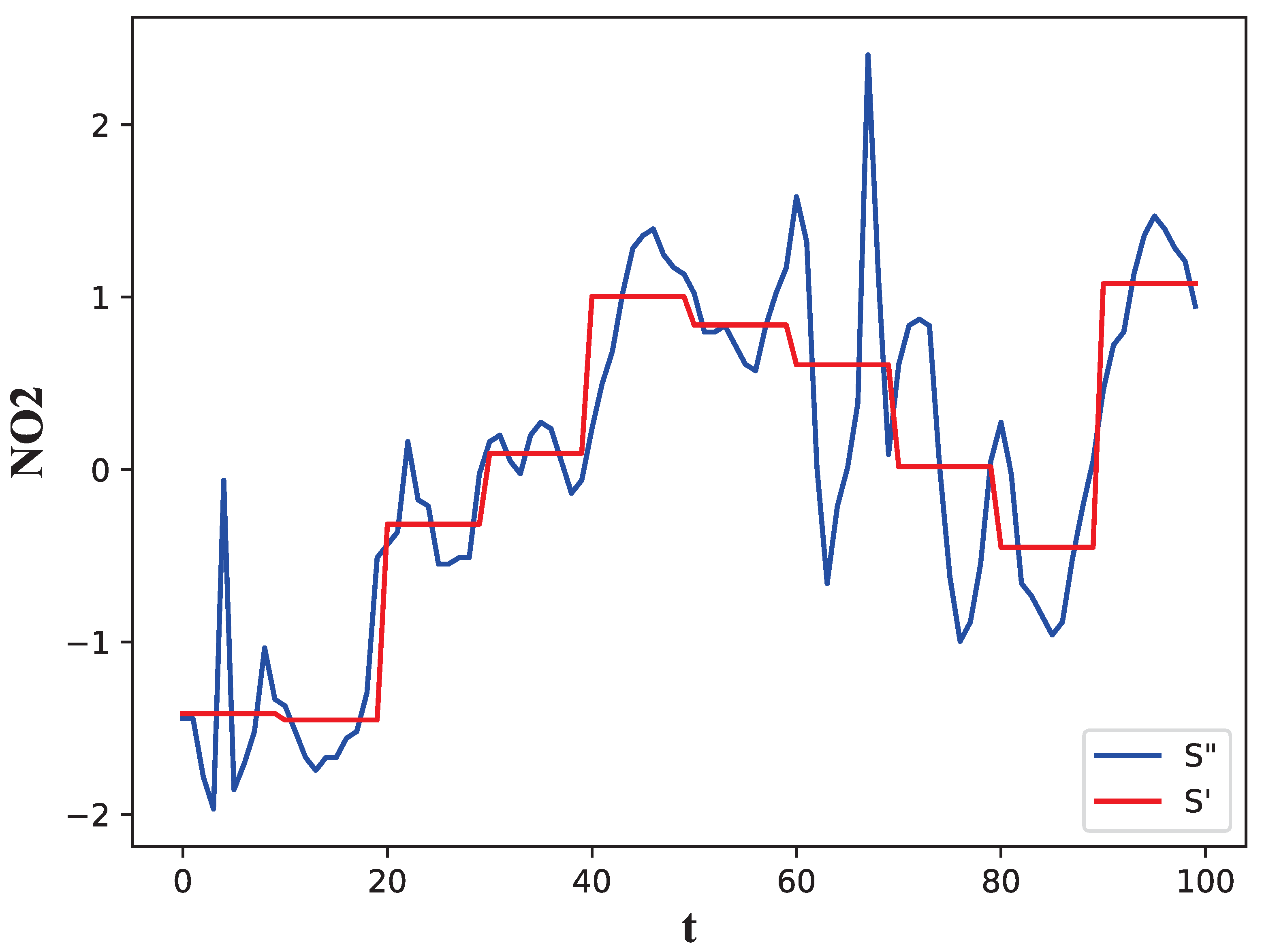
Figure 1 shows an example of the transition of NO${}_2$ from the original numerical MTS ($S^{{}^{″}}$) to the PAA version of MTS ($S^{{}^{\prime }}$). Here, $m=10$ and $M=100$. This way, the dimension is reduced from 100 to 10.

Figure 1. The original numerical MTS and PAA-MTS.

Definition 3.

The SAX-MTS $S=(T,A,V={\cup }_{a\in A}{V}_a,f)$ also has a similar form to Definition 2. The only difference is that the numerical value is transformed into a symbolic one. To produce symbols with equiprobability, a set of breakpoints $D=\{{\delta }_1,{\delta }_2,\cdots ,{\delta }_{g-1}\}$ dividing the area of under the probability distribution function (PDF) of $a\in A$ is required. Therefore, let $V_a=\{{\gamma }_1,{\gamma }_2,\cdots ,{\gamma }_g\}$ containing g symbols; then, we have:

$$f_{i,a}={\gamma }_j, if{f}_{i,a}^{{}^{\prime }}\in ({\delta }_{j-1},{\delta }_j),$$

(3)

where $j\in [1,g]$, and ${\delta }_0$, and ${\delta }_g$ are defined as $-\infty$ and $+\infty$, respectively.

Example 2.

Table 2 shows a lookup table of breakpoints for the $\mathcal{N}(0,1)$ distribution. In practice, g can be set as an integer that is not less than 2. Notably, $g=2$ means that $D=\left\{0\right\}$.

Table 2. The breakpoints for the $\mathcal{N}(0,1)$ distribution [52].

D	g
	3	4	5	6	7	8	9	10
${\delta }_1$	−0.43	−0.67	−0.84	−0.97	−1.07	−1.15	−1.22	−1.28
${\delta }_2$	0.43	0	−0.25	−0.43	−0.57	−0.67	−0.76	−0.84
${\delta }_3$		0.67	0.25	0	−0.18	−0.32	−0.43	−0.52
${\delta }_4$			0.84	0.43	0.18	0	−0.14	−0.25
${\delta }_5$				0.97	0.57	0.32	0.14	0
${\delta }_6$					1.07	0.67	0.43	0.25
${\delta }_7$						1.15	0.76	0.52
${\delta }_8$							1.22	0.84
${\delta }_9$								1.28

Example 3.

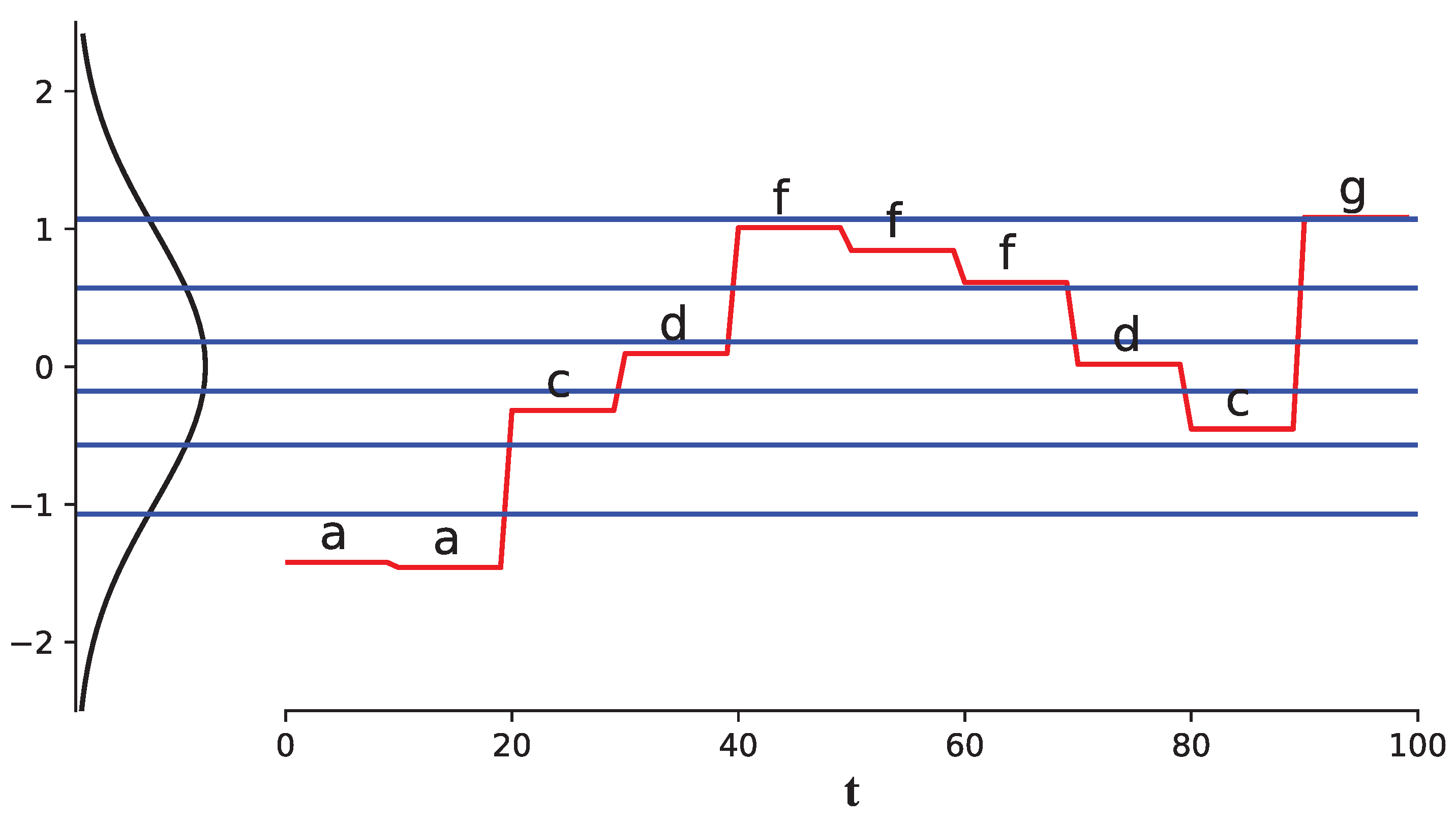
Figure 2 shows an example of the transition from PAA-MTS to SAX-MTS. Here, we let $D=\{-1.07,-0.57,-0.18,0.18,0.57,1.07\}$, $g=6$, and its alphabet $\Sigma =$ {a, b, c, d, e, f, g}.

Figure 2. The PAA-MTS and SAX-MTS for NO${}_2$.

Example 4.

Table 3 shows an example of SAX-MTS with three variables (i.e., $A=$ {SO${}_2$ ($a_1$), NO${}_2$ ($a_2$), and PM2.5 ($a_3$)}), and 10 time stamps (i.e., $T=\{t_1,t_2,\cdots ,t_{10}\}$). For variable SO${}_2$, symbols a and f are missing. For variable NO${}_2$, symbols b and e are missing. For variable PM2.5, symbols e, d, and e are missing. This phenomenon is temporary until the data are big enough.

Table 3. An example of SAX-MTS and PAA-MTS.

T	A
	SO${}_2$ $\left({\mathit{a}}_1\right)$	NO${}_2$ $\left({\mathit{a}}_2\right)$	PM2.5 $\left({\mathit{a}}_3\right)$
$20\left(t_1\right)$	b (−0.989)	a (−1.422)	b (−0.857)
$21\left(t_2\right)$	b (−0.966)	a (−1.460)	b (−0.770)
$22\left(t_3\right)$	b (−0.615)	c (−0.318)	b (−0.752)
$23\left(t_4\right)$	d (−0.106)	d (0.095)	b (−0.681)
$24\left(t_5\right)$	g (1.173)	f (1.007)	f (0.922)
$25\left(t_6\right)$	g (1.496)	f (0.842)	g (1.490)
$26\left(t_7\right)$	e (0.272)	f (0.609)	f (0.959)
$27\left(t_8\right)$	c (−0.203)	d (0.016)	c (−0.465)
$28\left(t_9\right)$	c (−0.508)	c (−0.453)	b (−0.691)
$29\left(t_{10}\right)$	e (0.447)	g (1.083)	f (0.846)

3.2. State

First, a formal description of the state is introduced as follows. Additionally, the type of prediction result that the SAX-MTS state is was described.

Definition 4.

Given a SAX-MTS $S=(T,A,V={\cup }_{a\in A}{V}_a,f)$: $\forall i\in [1,m]$,

$${\mathbf{f}}_{i,⁎}=(f_{i,1},f_{i,2},\cdots ,f_{i,n})$$

(4)

is called a state of SAX-MTS at time $t_i$. Moreover, the state of PAA-MTS (i.e, ${\mathbf{f}}_{i,⁎}^{{}^{\prime }}$=$(f_{i,1}^{{}^{\prime }},$$f_{i,2}^{{}^{\prime }},$$\cdots ,$$f_{i,n}^{{}^{\prime }})$) is formally similar to this one.

Example 5.

With Table 3, ${\mathbf{f}}_{10,⁎}=$ {e, g, f} is called a state of SAX-MTS at time $t_{10}$. Accordingly, ${\mathbf{f}}_{10,⁎}^{{}^{\prime }}=$ {0.447, 1.038, 0.846} is called a state of PAA-MTS at time $t_{10}$.

Second, the state ${\mathbf{f}}_{i,⁎}$ is denoted as a known label. This way, the corresponding instance of ${\mathbf{f}}_{i,⁎}$ is defined as follows.

Definition 5.

Given an SAX-MTS $S=(T,A,V,f)$ and a sliding window $w<m$, an instance with the matrix form is:

$$O_i^{w,n}=\left(\begin{array}{ccc}{f}_{i-w+1,1}& \dots & f_{i-w+1,n}\\ ⋮& \ddots & ⋮\\ f_{i,1}& \dots & f_{i,n}\end{array}\right)=({\mathbf{f}}_{⁎,1}^i,\dots ,{\mathbf{f}}_{⁎,n}^i)=\left(\begin{array}{c}{\mathbf{f}}_{i-w+1,⁎}^i\\ ⋮\\ {\mathbf{f}}_{i,⁎}^i\end{array}\right),$$

(5)

where $w\in (0,m)$, $i\in [w,m]$, and $\forall j\in [1,n]$, $|{\mathbf{f}}_{⁎,j}^i|=w$, $\forall j\in [i-w+1,i],|{\mathbf{f}}_{j,⁎}^i|=w$. For brevity, $O_i^{w,n}$ can be denoted by $O_i$ when n and w are specified:

Example 6.

With Table 3, let $w=2$ and $i=9$; then:

$$O_9=\left(\begin{array}{ccc}\mathrm{c}& \mathrm{d}& \mathrm{c}\\ \mathrm{c}& \mathrm{c}& \mathrm{b}\end{array}\right).$$

${\mathbf{f}}_{10,⁎}=$ {e, g, f} is the label of $O_9$.

This way, the set of all instances can be denoted by

$$\mathbf{SP}=\{O_w,O_{w+1},\cdots ,O_m\},$$

(6)

where $\left|\mathbf{SP}\right|=\left|T\right|-w=m-w+1$.

Example 7.

With Table 3, let $w=2$; then, $\mathbf{SP}=\{O_2,O_3,\cdots O_{10}\}$. Hence, $\left|\mathbf{SP}\right|=10-2+1=7$.

Third, $\forall i\in [w,m-1]$, the set of instance–label pair {($O_i$, ${\mathbf{f}}_{i+1,⁎}$)} can be constructed for the k-nearest matrix neighbors (kNMN).

Definition 6.

Given an instance $O_m\in \mathbf{SP}$, any $\mathbf{N}\subseteq \mathbf{SP}\backslash \left\{O_m\right\}$ is called the set of kNMN of $O_m$ if $\left|\mathbf{N}\right|=k$ and:

$$\underset{O^{{}^{\prime }}\in \mathbf{N}}{min}\Delta (O_m,O^{{}^{\prime }})\ge \underset{O^{{}^{″}}\in \mathbf{SP}\backslash \mathbf{N}}{max}\Delta (O_m,O^{{}^{″}}),$$

(7)

where Δ is the along–across similarity of the given matrix pair.

Note that the neighborhood $\mathbf{N}$ for $O_m$ may not be unique, where some other matrices have the same similarity with $O_m$.

Fourth, the along–across similarity model $\Delta$ is proposed to obtain the neighborhood $\mathbf{N}$ by merging the popular similarity and distance metrics.

Definition 7.

Given PAA-MTS $S^{{}^{\prime }}=(T,A,V^{{}^{\prime }},f^{{}^{\prime }})$, SAX-MTS $S=(T,A,V,f)$, and sliding window size w, the similarity between the two matrix-based instances $O_i$ and $O_j$ is:

$$\Delta (O_i,O_j)=R_{i,j}\times C_{i,j},$$

(8)

where the row vector similarity is:

$$R_{i,j}=\frac{{\sum }_{l=1}^{w}s({\mathbf{h}}_{i-w+l,⁎}^i,{\mathbf{h}}_{j-w+l,⁎}^j)}{w},$$

(9)

and the column vector similarity is:

$$C_{i,j}=\frac{{\sum }_{l=1}^{n}s({\mathbf{h}}_{⁎,l}^i,{\mathbf{h}}_{⁎,l}^j)}{n},$$

(10)

where:

$$\begin{array}{c}\hfill \mathbf{h}=\left\{\begin{array}{cc}{\mathbf{f}}^{{}^{\prime }},\hfill & ifthemetricisavailableforthePAA-MTS;\hfill \\ \mathbf{f},\hfill & ifthemetricisavailablefortheSAX-MTS.\hfill \end{array}\right.\end{array}$$

(11)

Note that the row or column vector $\mathbf{h}$ in Equation (11) is indeed one of ${\mathbf{f}}^{{}^{\prime }}$ and $\mathbf{f}$, corresponding to PAA- and SAX-MTSs, respectively. Moreover, the data type of vector $\mathbf{h}$ in Equations (9) and (10) are coincident. In other words, the pairs of vectors in Equations (9) and (10) are either PAA-MTS or SAX-MTS. Namely, the case that ${\mathbf{h}}_{⁎,l}^i$ is PAA-MTS while ${\mathbf{h}}_{⁎,l}^j$ is SAX-MTS is not permitted.

Table 4 presents the availability of similarities and distances for Equation (11). Two things need to be further explained. One is the availability of the metrics. Given any two indices r and c ($r,c\in$ IDs), PAA(r) = True or PAA(c) = True indicates that the r-th or the c-th metric fits the numerical data. Similarly, SAX(r) = True or SAX(c) = False means that the r-th or the c-th metric fits the symbolic data. For example, PAA(0) = True indicates that the Euclidean distance fits PAA-MTS but not SAX-MTS.

Table 4. The availability of similarities and distances.

IDs	Name	Type	Availability
			PAA	SAX
0	Euclidean	distance	True	False
1	Manhattan	distance	True	False
2	LCSubstring [53]	distance	False	True
3	Levenshtein [54]	distance	False	True
4	Cosine	similarity	True	False
5	Pearson	similarity	True	False
6	Tanimoto [55]	similarity	True	False
7	Triangle [56]	similarity	True	False
8	Jaccard	similarity	False	True
9	Jaro	similarity	False	True

The other is the transformation from the distance to similarity. As similarity and distance metrics are simultaneously used here, the distance needs be transformed into the similarity. Therefore, given two vectors ${\mathbf{h}}^i$ and ${\mathbf{h}}^j$, the transformation from distance to similarity is:  

$$s({\mathbf{h}}^i,{\mathbf{h}}^j)=\frac{1}{d({\mathbf{h}}^i,{\mathbf{h}}^j)+1},$$

(12)

where d denotes the distance between ${\mathbf{h}}^i$ and ${\mathbf{h}}^j$. This way, 100 combinations of distances and similarities exist. Their performances are discussed in Section 5.

Example 8.

With Table 3 and Table 4, let $r=8$ (Jaccard similarity, PAA$\left(8\right)=$ True), $c=1$ (Manhattan distance, SAX$\left(1\right)=$ True), and $w=2$, and the along–across similarity between $O_6$ and $O_7$ (i.e., $\Delta (O_6,O_7)$) is illustrated as follows. First, the SAX-MTS and PAA-MTS of $O_6$ is:

$$O_6=\left(\begin{array}{ccc}g& f& f\\ g& f& g\end{array}\right),and\left(\begin{array}{ccc}1.173& 1.007& 0.922\\ 1.496& 0.842& 1.490\end{array}\right),respectively.$$

Those of $O_7$ is:

$$O_7=\left(\begin{array}{ccc}g& f& g\\ e& f& f\end{array}\right),and\left(\begin{array}{ccc}1.496& 0.842& 1.490\\ 0.272& 0.609& 0.959\end{array}\right),respectively.$$

Second, the row vector similarity $R_{6,7}=\frac{\frac{2}{3}+\frac{1}{3}}{2}=0.5$. More specifically, the Jaccard similarity between row vectors (g, f, f) and (g, f, g) is $\frac{2}{3}$. Third, the column similarity $C_{6,7} =$$\frac{\frac{1}{1.547+1}+\frac{1}{0.398+1}+\frac{1}{1.099+1}}{3}$$= \frac{0.393+0.715+0.476}{3}$$= 0.528$. More specifically, the Manhattan distance between column vectors $(1.173,1.496)$ and $(1,496,0.272)$ is $0.323+1.224=1.547$. Finally, $\Delta (O_6,O_7)$$= 0.5\times 0.528$$= 0.264$.

Fifth, given a future time stamp (e.g., $t_{11}$), the state (e.g., ${\mathbf{f}}_{11}$) at this time is unknown. Formally, the state occurring at time $t_{m+1}$ is denoted as ${\mathbf{p}}_{m+1}$=$(p_{m+1,1}$, $p_{m+1,2}$, ⋯, $p_{m+1,n})$. To obtain the components of ${\mathbf{p}}_{m+1,⁎}$ with the kNN-like method, the instances, neighbors, and labels were defined by the above. Therefore, the label of $O_m$, i.e., ${\mathbf{p}}_{m+1,⁎}$ can be predicted with the following voting strategy.

Definition 8.

Given a SAX-MTS $S=(T,A,V,f)$, $O_m$ and $\mathbf{N}$, $\forall j\in [1,n]$, each component of ${\mathbf{p}}_{m+1,⁎}=(p_{m+1,1},p_{m+1,2},\cdots ,p_{m+1,n})$ is:

$$p_j=arg\underset{v_{a_j}\in V_{a_j}}{max}vote\left(v_{a_j}\right),$$

(13)

and:

$$vote\left(v_{a_j}\right)=\frac{{\sum }_{i\in \left\{i\right|O_i\in \mathbf{N}\}}I(v_{a_j}=f_{i+1,j})}{\left|\mathbf{N}\right|},$$

(14)

where $I(·)=1$, if the condition $(·)$ is True; otherwise, $I(·)=0$.

Example 9.

With Table 3 and Table 4, let $r=8$, $c=2$, and $w=2$, the process of computing ${\mathbf{p}}_{11,⁎}=(p_{11,1}, p_{11,2}, p_{11,3})$ is illustrated as follows.

First, the $\mathbf{N}$ of $O_{10}$ is found. Using the process shown in Example 8, the along–across similarities of $\left\{O_{10}\right\}\times \{O_2,O_3,\cdots ,O_9\}$ are listed in Table 5. Let the size of $\mathbf{N}$, i.e., $k=4$; then, $\mathbf{N}$$= \{O_5,$$O_4,$$O_7,$$O_6\}$.

Table 5. The similarity matrix of $O_{10}$.

	${\mathit{O}}_2$	${\mathit{O}}_3$	${\mathit{O}}_4$	${\mathit{O}}_5$	${\mathit{O}}_6$	${\mathit{O}}_7$	${\mathit{O}}_8$	${\mathit{O}}_9$
$O_{10}$	0.051	0.059	0.243	0.334	0.105	0.109	0	0.063

Second, with the three nearest neighbors, the states/labels after them can be obtained. Namely, ${\mathbf{f}}_{6,⁎}=$ (g, f, g), ${\mathbf{f}}_{5,⁎}=$ (g, f, f), ${\mathbf{f}}_{8,⁎}=$ (c, d, c), and ${\mathbf{f}}_{7,⁎}=$ (e, f, f).

Fourth, the results of voting can hence be obtained as $p_{11,1}=$ g, $p_{11,2}=$ f, $p_{11,3}=$ f. Namely, ${\mathbf{p}}_{11,⁎}=$ (g, f, f). More specially, in terms of $a_1$, $vote\left(g\right)=2>vote\left(c\right)=1=vote\left(e\right)$.

Sixth, the prediction performance is better with less difference between the ${\mathbf{p}}_{m+1,⁎}$ and ${\mathbf{f}}_{m+1,⁎}$ in general. The measures of prediction performance such as the precision and recall are introduced here. $\forall i\in [1,n]$, and the precision and recall of the state ${\mathbf{f}}_{m+1,⁎}$ have the same form, namely:

$${\mathcal{P}}_{m+1}=\frac{{\Sigma }_{1\le i\le n}I(p_{m+1,i}==f_{m+1,i})}{n}$$

(15)

Finally, with the above definitions, the problem of state prediction is proposed as follows.

Problem 1.

kNMN-based state prediction for MTS:

Input:  $S^{{}^{\prime }}=(T,A,V^{{}^{\prime }},f^{{}^{\prime }})$, $S=(T,A,V,f)$, w and k;

Output:  ${\mathbf{p}}_{m+1,⁎}=(p_{m+1,1},p_{m+1,2},\cdots ,p_{m+1,n}).$

Although two types of datasets, i.e., the PAA- and SAX-MTSs, are both used here, the space complexity remains the same. The time complexity is closely related to the size of the matrix instance and similarity metrics for vectors.

Example 10.

With Table 4, let $r=8$ and $c=2$; given PAA-MTS $S^{{}^{\prime }}$, SAX-MTS S, and the sliding window w, the time complexities of the row and column vectors’ similarity between two matrix instances are both $\Theta \left(wn\right)$. Moreover, the size of $\mathbf{SP}$ is $n-w+1$; hence, the time complexity of our method is $\Theta \left(wn\right(m-w+1\left)\right)=\Theta \left(mn\right)$.

3.3. Tri-State

To enrich the semantics of predictions, we extend each component of ${\mathbf{p}}_m$ to a column vector with length 3. For each vector, different components have various semantics. This way, the form of prediction is changed from a $1\times n$ vector into a $3\times n$ matrix.

First, we introduce the definition of the tri-partition alphabet as follows.

Definition 9.

Given an SAX-MTS $S=(T,A,V,f)$, $\forall a\in A$,

$${\Sigma }_a=({\Gamma }_a,{\Lambda }_a,{\Omega }_a)$$

(16)

is called a tri-partition alphabet of a if

• ${\Gamma }_a\cup {\Lambda }_a\cup {\Omega }_a={\Sigma }_a=V_a$; and
• ${\Gamma }_a\cap {\Lambda }_a={\Gamma }_a\cap {\Omega }_a={\Omega }_a\cap {\Lambda }_a=Ø$.

Additionally, we call ${\Gamma }_a$, ${\Lambda }_a$, and ${\Omega }_a$ the strong, medium, and weak regions of attribute $a\in A$, respectively.

Example 11.

With Table 3, the range of values for variable NO${}_2$ ($a_2$) is {a, b, c, d, e, f, g}. Let ${\Gamma }_{a_2}=$ {a, g}, ${\Lambda }_{a_2}=$ {b, f}, and ${\Omega }_{a_2}=$ {c, d, e}, ${\Sigma }_{a_2}$ is called a tri-partition alphabet of NO${}_2$.

Definition 10.

Given a SAX-MTS $S=(T,A,V={\cup }_{a\in A}{V}_a,f)$: $\Sigma ={\cup }_{a\in A}{\Sigma }_a$ and $O_m$, a tri-state at time stamp $t_{m+1}$ is:

$$P_{m+1,*}=\left(\begin{array}{ccc}{p}_{m+1,1}^{{\Gamma }_{a_1}},& \dots ,& p_{m+1,n}^{{\Gamma }_{a_n}}\\ p_{m+1,1}^{{\Lambda }_{a_1}},& \dots ,& p_{m+1,n}^{{\Lambda }_{a_n}}\\ p_{m+1,1}^{{\Omega }_{a_1}},& \dots ,& p_{m+1,n}^{{\Omega }_{a_n}}\end{array}\right)$$

(17)

where $\forall i\in [1,n]$, $p_{m+1,i}^{{\Gamma }_{a_i}}\in {\Gamma }_i$, $p_{m+1,i}^{{\Lambda }_{a_i}}\in {\Lambda }_i$, and $p_{m+1,i}^{{\Omega }_{a_i}}\in {\Omega }_i$.

Compared with the state in Definition 4, we replace $p_{m+1,i}$ with ${\mathbf{p}}_{m+1,i}$$= (p_{m+1,i}^{{\Gamma }_{a_i}}$, $p_{m+1,i}^{{\Lambda }_{a_i}}$, $p_{m+1,i}^{{\Omega }_{a_i}}{)}^{\mathrm{T}}$, $\forall i\in [1,n]$. Moreover, this predicted vector can be interpreted as the most probable symbol from the strong, medium, and weak regions, respectively. Note that the three-way state is useless for historical data.

Therefore, we present the voting strategy for the three-way state prediction as follows. Given $\forall i\in [1,n]$:

$$\begin{array}{c}\hfill \left\{\begin{array}{c}{p}_{m+1,i}^{{\Gamma }_{a_i}}=arg\underset{v_{a_i}\in {\Gamma }_{a_i}}{max}vote\left(v_{a_i}\right);\hfill \\ p_{m+1,i}^{{\Lambda }_{a_i}}=arg\underset{v_{a_i}\in {\Lambda }_{a_i}}{max}vote\left(v_{a_i}\right);\hfill \\ p_{m+1,i}^{{\Omega }_{a_i}}=arg\underset{v_{a_i}\in {\Omega }_{a_i}}{max}vote\left(v_{a_i}\right).\hfill \end{array}\right.\end{array}$$

(18)

Practically, regions ${\Gamma }_a$, ${\Lambda }_a$, and ${\Omega }_a$ can be obtained using various partition strategies and have meaningful explanations. Here, we partition the range of symbolic values for each attribute using the following strategy. Based on Equations (2) and (3), we can evaluate the level deviating from the mean for each symbol. For each attribute $a_i(i\in [1,n])$, given a set of thresholds pair $\left\{({\alpha }_i,{\beta }_i)\right\}$ with cardinality n, where ${\alpha }_i,{\beta }_i\in D=\{{\delta }_1,{\delta }_2,\cdots ,{\delta }_{g-1}\}$, ${\alpha }_i\ge {\beta }_i>0$. $\forall j\in [1,g-1]$, the tri-partition strategy is formally described as

$$\begin{array}{c}\hfill \left\{\begin{array}{cc}{\gamma }_{i,j}\in {\Gamma }_{a_i},\hfill & \mathrm{if}|{\delta }_j|\ge {\alpha }_i;\hfill \\ {\gamma }_{i,j}\in {\Lambda }_{a_i},\hfill & \mathrm{if}{\alpha }_i>\left|{\delta }_j\right|\ge {\beta }_i;\hfill \\ {\gamma }_{i,j}\in {\Omega }_{a_i},\hfill & \mathrm{if}|{\delta }_j|<{\beta }_i.\hfill \end{array}\right.\end{array}$$

(19)

The combination of PAA-MTS $S^{{}^{\prime }}=(T,A,V^{{}^{\prime }},f^{{}^{\prime }})$ and SAX-MTS $S=(T,A,V,f)$ is first used here. The breakpoint ${\delta }_g$ is $+\infty$, and ${\delta }_g>\alpha$ always holds. Hence, ${\gamma }_g$ always belongs to ${\Gamma }_{a_i}$.

However, up to $2n$ thresholds need to be specified. Therefore, we assume that $\forall i,j\in [1,n],i\ne j$, ${\alpha }_i={\alpha }_j$, and ${\beta }_i={\beta }_j$ for brevity. Consequently, we have ${\Sigma }_{a_i}={\Sigma }_{a_j}$, and $\Sigma =\{{\Sigma }_a=({\Gamma }_a,{\Lambda }_a,{\Omega }_a)|a\in A\}$ which can be denoted by $\Sigma =(\Gamma ,\Lambda ,\Omega )$. More choices are available for $\alpha$ and $\beta$ with a greater g. Moreover, if $g=4$, then $D=\{-0.67,0,0.67\}$. When the threshold $\alpha$ is set to $0.67$, $\beta$ can be set to $0.67$ or 0.

However, the predicted tri-state is incomplete if no strong, medium, or weak symbols are found following the whole matrix neighbors. Namely, what the current method can guarantee is that each variable has at least one predicted symbol. Formally, given a tri-state $P_{m+1,⁎}$ at $t_{m+1}$, $\forall i\in [1,n]$, we have:

$${(p_i^{\Gamma },p_i^{\Lambda },p_i^{\Omega })}^{\mathrm{T}}\ne {(\varphi ,\varphi ,\varphi )}^{\mathrm{T}}.$$

Example 12.

With Table 3, let $\alpha =1.07$ and $\beta =0.57$, ${\Sigma }_{a_1}={\Sigma }_{a_2}={\Sigma }_{a_3}=(\Gamma ,\Lambda ,\Omega )$, where $\Gamma =$ {a, g}, $\Lambda =$ {b, f} and $\Omega =$ {c, d, e}. Based on the four labels of Example 9, i.e., ${\mathbf{f}}_{6,⁎}=$ (g, f, g), ${\mathbf{f}}_{5,⁎}=$ (g, f, f), ${\mathbf{f}}_{8,⁎}=$ (c, d, c), and ${\mathbf{f}}_{7,⁎}=$ (e, f, f), the predicted tri-state at $t_{11}$ is $P_{11,⁎}=\left(\begin{array}{ccc}g,& \varphi ,& g\\ \varphi ,& f,& f\\ \mathrm{c/e},& d,& c\end{array}\right).$

Note that ϕ means the symbol of the current position is temporally unknown. More specifically, the strong symbol of $a_2$ and the medium symbol of $a_1$ are unknown. Here, “c / e” indicates that the final predicted symbol was randomly selected from them. For brevity, the symbol c was selected.

Moreover, the precision for the incomplete tri-state is calculated as follows:

$${\mathcal{P}}_{m+1}^{{}^{\prime }}=\frac{{\Sigma }_{1\le i\le n}I(p_{m+1,i}^{\Gamma }==f_{m+1,i}\mathrm{or}{p}_{m+1,i}^{\Lambda }==f_{m+1,i}\mathrm{or}{p}_{m+1,i}^{\Omega }==f_{m+1,i})}{{\Sigma }_{i\in [1,n]}{\Sigma }_{j\in [1,3]}I(P_{m+1,⁎}\ne \varphi )}$$

(20)

In order to remedy this defect, i.e., to obtain a completed tri-state, we propose two simplified and effective filling strategies called the individual and related ones, respectively. For each attribute, if one or two symbols are missing, the individual filling strategy (IFS) predicts them with the most frequent ones in its own history data. Then, $\forall i\in [1,n]$, the IFS can be formally described as follows:

$$\begin{array}{c}\hfill \left\{\begin{array}{cc}{p}_i^{\Gamma }={arg}_{\gamma \in \Gamma }max\mathrm{IFS}-\mathrm{Count}\left(\gamma \right),\hfill & \mathrm{if}{p}_i^{\Gamma }=\varphi ;\hfill \\ p_i^{\Lambda }={arg}_{\gamma \in \Lambda }max\mathrm{IFS}-\mathrm{Count}\left(\gamma \right),\hfill & \mathrm{if}{p}_i^{\Lambda }=\varphi ;\hfill \\ p_i^{\Omega }={arg}_{\gamma \in \Omega }max\mathrm{IFS}-\mathrm{Count}\left(\gamma \right),\hfill & \mathrm{if}{p}_i^{\Omega }=\varphi ,\hfill \end{array}\right.\end{array}$$

(21)

where:

$$\mathrm{IFS}-\mathrm{Count}\left(\gamma \right)=\frac{{\Sigma }_{j=1}^m\mathrm{Index}(f_{j,i}=\gamma )}{m}.$$

Example 13.

According to Example 12 and Table 3, for variable $a_1$, $p_1^{\Lambda }=$ b. This is because IFS-Count(b) = $\frac{3}{10}$ > IFS-Count(f) = 0. For variable $a_2$, $p_2^{\Gamma }=$ a. This is because IFS-Count(a) = $\frac{2}{10}$ > IFS-Count(g) = $\frac{1}{10}$. Hence, the tri-state filled by the IFS is $P_{11,⁎}=\left(\begin{array}{ccc}g,& a,& g\\ b,& f,& f\\ c,& d,& c\end{array}\right).$

The related filling strategy (RFS) predicts the missing symbols by considering the association relationships between any pair of variables. Given two variables $a_i$ and $a_j$ ($i,j\in [1,n],i\ne j$), $a_j$ is the most linear related variable of $a_i$. Namely, $a_j={arg}_{a_j\in A\backslash \left\{a_i\right\}}\max \mathrm{Pearson}(a_i,a_j)$. Hence, their predicted vectors are ${(p_i^{\Gamma },p_i^{\Lambda },p_i^{\Omega })}^{\mathrm{T}}$ and ${(p_j^{\Gamma },p_j^{\Lambda },p_j^{\Omega })}^{\mathrm{T}}$. Then, the RFS can be formally described as follows:

$$\begin{array}{c}\hfill \left\{\begin{array}{cc}{p}_i^{\Gamma }={arg}_{\gamma \in \Gamma }max\mathrm{RFS}-\mathrm{Count}\left(\gamma \right),\hfill & \mathrm{if}{p}_i^{\Gamma }=\varphi ;\hfill \\ p_i^{\Lambda }={arg}_{\gamma \in \Lambda }max\mathrm{RFS}-\mathrm{Count}\left(\gamma \right),\hfill & \mathrm{if}{p}_i^{\Lambda }=\varphi ;\hfill \\ p_i^{\Omega }={arg}_{\gamma \in \Omega }max\mathrm{RFS}-\mathrm{Count}\left(\gamma \right),\hfill & \mathrm{if}{p}_i^{\Omega }=\varphi ,\hfill \end{array}\right.\end{array}$$

(22)

where:

$$\mathrm{RFS}-\mathrm{Count}\left(\gamma \right)=\frac{{\Sigma }_{{\gamma }^{{}^{\prime }}\in \{p_i^{\Gamma },p_i^{\Lambda },p_i^{\Omega }\}}{\Sigma }_{l=1}^m\mathrm{Index}(f_{l,i}=\gamma \mathrm{and}{f}_{l,j}={\gamma }^{{}^{\prime }}\mathrm{and}{f}_{l,j}\ne \varphi )}{{\Sigma }_{{\gamma }^{{}^{\prime }}\in \{p_i^{\Gamma },p_i^{\Lambda },p_i^{\Omega }\}}\mathrm{Index}({\gamma }^{{}^{\prime }}\ne \varphi )\times m}.$$

Example 14.

Based on Example 12 and Table 3, the Pearson correlations among the three variables are listed as follows. Pearson$(a_1,a_2)=0.892$, Pearson$(a_1,a_3)=0.919$, and Pearson$(a_2,a_3)=0.839$. Hence, for the variable $a_1$, the most related one is $a_3$. Then, when ($a_3$, g) happens, the happening symbols set of $a_1$ is {g}. When ($a_3$, f) happens, the happening symbols set of $a_1$ is {g, e, e}. When ($a_3$, c) happens, the happening symbols set of $a_1$ is {c}. No medium symbol for $p_1^{\Lambda }$ by the RFS is available. Therefore, the result is b, which is predicted using the IFS.

Then, for the variable $a_2$, the most related one is $a_1$. Then, when ($a_1$, g) happens, the happening symbols’ set of $a_2$ is {f, f}. When ($a_1$, b) happens, the happening symbols set of $a_2$ is {a, a, c}. When ($a_1$, c) happens, the happening symbols set of $a_2$ is {d, c}. Therefore, the result of $p_i^{\Gamma }$ is a.

Accordingly, the tri-state filled by the RFS is $P_{11,⁎}=\left(\begin{array}{ccc}g,& a,& g\\ b,& f,& f\\ c,& d,& c\end{array}\right).$ This result of the RFS is consistent with that of the IFS.

Moreover, the precision for the completed tri-state (IFS- and RFS-ones) is calculated as follows:

$${\mathcal{P}}_{m+1}^{{}^{″}}=\frac{{\Sigma }_{1\le i\le n}I(p_{m+1,i}^{\Gamma }==f_{m+1,i}\mathrm{or}{p}_{m+1,i}^{\Lambda }==f_{m+1,i}\mathrm{or}{p}_{m+1,i}^{\Omega }==f_{m+1,i})}{3n}$$

(23)

With the above Equations (15), (20) and (23):

• $0\le {\mathcal{P}}_{m+1}^{{}^{″}}\le \frac{1}{3}$;
• ${\mathcal{P}}_{m+1}^{{}^{\prime }}\le {\mathcal{P}}_{m+1}$; and ${\mathcal{P}}_{m+1}^{{}^{″}}\le {\mathcal{P}}_{m+1}$.

Finally, with all of the above definitions, we can define the problem of three-way state prediction as follows:

Problem 2.

Tri-state prediction for MTS.

Input:  $S^{{}^{\prime }}=(T,A,V^{{}^{\prime }},f^{{}^{\prime }})$, $S=(T,A,V,f)$, w, k, α, and β;

Output:  $P_{m+1,⁎}=({\mathbf{p}}_{m+1,n},{\mathbf{p}}_{m+1,n},\dots ,{\mathbf{p}}_{m+1,n})=\left(\begin{array}{ccc}{p}_{m+1,1}^{\Gamma },& \dots ,& p_{m+1,n}^{\Gamma }\\ p_{m+1,1}^{\Lambda },& \dots ,& p_{m+1,n}^{\Lambda }\\ p_{m+1,1}^{\Omega },& \dots ,& p_{m+1,n}^{\Omega }\end{array}\right).$

Compared with Problem 1, Problem 2 has two more parameters α and β. The first process that generates Σ is required, but it has a polynomial time complexity $\Theta \left(mn\right)$. The output is a matrix P with size $3\times n$. Hence, we can obtain three of the most likely occurring symbols from the strong, medium, and weak regions, respectively. Note that Problem 1 obtains one predicted state at once, while Problem 2 can obtain up to $3^n$ possible states. Excitedly, the time and space complexity of the two problems remain the same.

4. Algorithms

In this section, the framework of the three-way state prediction algorithm with k nearest matrix neighbors (kNMN-3WSP) is shown in Figure 3. Three stages, namely kNMN construction, alphabet tri-partition, and three-way state prediction, are proposed. Note that datasets such as PAA $S^{{}^{\prime }}$ and SAX S are the inputs of all stages. In stages II and III, $S^{{}^{\prime }}$ and S were omitted for brevity.

Figure 3. The process of the kNMN-3WSP algorithm.

4.1. Stage I

Algorithm 1 proposes the details of Stage I. First, $(r,c)$ is a pair of indexes which identifies the distances and similarities from Table 4. In other words, we have $r,c\in \{0,1,\dots ,9\}$. Moreover, if $r=0$, the similarity between two row vectors is measured using the Euclidean distance. If $c=7$, the similarity between two column vectors are measured using the Triangle one. Second, the cardinalities of $O_m$ and all elements in $\mathbf{SP}$ are $w\times n$, $\left|\mathbf{N}\right|=k$ and $m=\left|T\right|$. Third, the availability of PAA and SAX is the key to integrating $S^{{}^{\prime }}$ and S. They are mutually exclusive.

Algorithm 2 presents the details of Line 4. With the last two columns of Table 4, if the similarity metric supports PAA-MTS, PAA(r) or PAA(c) is True (T). For example, PAA(0) = PAA(1) = True, and PAA(2) = PAA(3) = False (F). Finally, the time complexity of this stage is $\Theta \left(m{n}^2\right)$.

Algorithm 1kNMN construction.

Input:  $S^{{}^{\prime }}=(T,A,V^{{}^{\prime }},f^{{}^{\prime }})$, $S=(T,A,V,f)$, w, k and $(r,c)$;

Output:  $\mathbf{N}$;

Method: Construction.

1: Generate $O_m$ and $\mathbf{SP}$ with w;   2: Initialize $\mathbf{N}=Ø$;   3: for ($i\in [w,m-1]$) do   4:     Compute $\Delta (O_m,O_i)$ with $(r,c)$;   5:     $\mathbf{N}=\mathbf{N}\cup \left(\{O_i,\Delta (O_m,O_i))\right\}$;   6: end for   7: Arrange the elements in set $\mathbf{N}$ in descending order of similarity $\Delta$;   8: Retain only the first k elements of $\mathbf{N}$;   9: return$\mathbf{N}$

Algorithm 2 Similarity computation.

Input:  $O_m$, $O_i$ and $(r,c)$;

Output:  $\Delta (O_m,O_i)$;

Method:  Similarity.

1: row = 0.0;   2: for ($l\in [1,w]$) do   3:     if (PAA$\left(r\right)$) then   4:         row += $s({\mathbf{f}\prime \hspace{0.17em}}_{m-w+l,*}^m,{\mathbf{f}\prime \hspace{0.17em}}_{i-w+l,*}^i)$;   5:     else   6:         row += $s({\mathbf{f}}_{m-w+l,*}^m,{\mathbf{f}}_{i-w+l,*}^i)$;   7:     end if   8: end for   9: row /= w;   10: col = 0.0;   11: for ($l\in [1,n]$) do   12:     if (PAA$\left(c\right)$) then   13:         col += $s({{\mathbf{f}\prime \hspace{0.17em}}^i}_{*,l},{{\mathbf{f}\prime \hspace{0.17em}}^j}_{*,l})$;   14:     else   15:         col += $s({\mathbf{f}}_{*,l}^i,{\mathbf{f}}_{*,l}^j)$;   16:     end if   17: end for   18: col /= n;   19: return row × col;

4.2. Stage II

Algorithm 3 describes the details of Stage II. First, the variable g was specified to generate the SAX version of MTS. In other words, $g\ge 2$ is the number of symbols for each attribute. Second, if $\alpha =\beta$, Λ is an Ø. When $g=2$, no other choices are available except for $\alpha =\beta$. Finally, the time complexity of this stage is only $\Theta \left(ng\right)$.

Algorithm 3 Alphabet tri-partition.

Input:  $S^{{}^{\prime }}=(T,A,V^{{}^{\prime }},f^{{}^{\prime }})$, $S=(T,A,V,f)$, $\alpha$ and $\beta$;

Output:  $\Sigma =(\Gamma ,\Lambda ,\Omega )$;

Method:  Tri-partition.

1: Initialize $\Gamma =\Lambda =\Omega =Ø$;   2: for ($i\in [1,g-1]$) do   3:     if $\left(\right|{\delta }_i|\ge \alpha$) then   4:         $\Gamma =\Gamma \cup \left\{{\gamma }_i\right\}$;   5: else if  $\left(\right|{\delta }_i|<\beta )$ then   6:         $\Omega =\Omega \cup \left\{{\gamma }_i\right\}$;   7:     else   8:         $\Lambda =\Lambda \cup \left\{{\gamma }_i\right\}$;   9:     end if   10: end for   11: $\Gamma =\Gamma \cup \left\{{\gamma }_g\right\}$;   12: return  $\Sigma =(\Gamma ,\Lambda ,\Omega )$;

4.3. Stage III

Algorithm 4 discusses the details of Stage III. First, $f_{j+1,i}$ is the label of attribute $a_i$. The predicted symbol is the one with the maximal frequency. Second, the purpose of using the index to count is to improve the efficiency of this algorithm. In Line 6, Count$(·)$ is a mapping function for the count matrix in which the size is $g\times 2$. The l-th position stores the frequency of ${\gamma }_l$ ($l\in [1,g]$). Generally, the matrix is denoted by $\mathbf{M}$ = ((Count(1), $1)$, (Count(2), $2)$, ⋯, (Count(g), $g)$). For example, with Table 3, let the indices of H, M, and L be 0, 1, and 2, respectively, ($g=3$). Matrix ((3, 0), (2, 1), (4, 2)) means the frequencies of H, M, and L are 3, 2, and 4, respectively. Moreover, ${\mathbf{M}}_{1,⁎}$ = (3, 0), ${\mathbf{M}}_{1,1}$ = 3, and ${\mathbf{M}}_{1,2}$ = 0.

In Line 9, the count matrices are listed in the count descending order. Generally, ${\mathbf{M}}^{\prime }=({\mathbf{M}}_{1,⁎},{\mathbf{M}}_{2,⁎},\cdots ,{\mathbf{M}}_{g,⁎})$ are subject to (1) $\forall i\in [1,g]$, ${\mathbf{M}}_{i,⁎}\in \mathbf{M}$, and (2) $\forall j\in [1,g],j\ne i$, ${\mathbf{M}}_{i,1}\ge {\mathbf{M}}_{j,1}$. For example, the matrix ((3, 0), (2, 1), (4, 2)) is transformed into ((4, 2), (3, 0), (2, 1)). In Lines 10–21, the algorithm searches for three symbols with the biggest count from the strong, medium, and weak regions each. There is no need to continue searching if all three symbols of the current variable are known. The time complexity of this stage is $\Theta \left(mn\right)$.

Finally, the RFS considers more information than the IFS, but their time and space complexities are the same, namely $\Theta \left(nm\right)$. This way, we can obtain four kinds of states called the state, tri-state, IFS-based tri-state (IFS-tri-state), and RFS-based tri-state (RFS-tri-state).

Algorithm 4 Three-way state prediction.

Input:  $S^{{}^{\prime }}=(T,A,V^{{}^{\prime }},f^{{}^{\prime }})$, $S=(T,A,V,f)$, N and $\Sigma =(\Gamma ,\Lambda ,\Omega )$;

Output:  $P^{3\times n}=\left(\begin{array}{ccc}{p}_1^{\Gamma },& \cdots ,& p_n^{\Gamma }\\ p_1^{\Lambda },& \cdots ,& p_n^{\Lambda }\\ p_1^{\Omega },& \cdots ,& p_n^{\Omega }\end{array}\right)$;

Method:  Prediction.

1: Initialize $P^{3\times n}$ by filling with $\varphi$;   2: for ($i\in [1,n]$) do   3:     M = ((Count(1), 1), (Count(2), 2), ⋯, (Count$\left(g\right)$, g)), Count$\left(l\right)=0$$(l\in [1,g\left]\right)$;   4:     for (each neighbor $O\in \mathbf{N}$) do   5:         Get its last time stamp, denoted by $t_j$;   6:         Obtain the index of $f_{j+1,i}$ in $V_{a_i}$, denoted by l;   7:         Count$\left(l\right)++$;   8:     end for   9:     Obtain ${\mathbf{M}}^{\prime }$ by listing M in the descending order of Count(·);   10:     for ($j\in [1,g]$) do   11:         Let $l={\mathbf{M}}_{j,2}^{\prime }$;   12:         if $({\gamma }_l\in \Gamma$ and $p_i^{\Gamma }\ne \varphi$) then   13:             $p_i^{\Gamma }={\gamma }_l$;   14:         else if $({\gamma }_l\in \Lambda )$ and $p_i^{\Lambda }\ne \varphi$ then   15:             $p_i^{\Lambda }={\gamma }_l$;   16:         else if $({\gamma }_l\in \Omega )$ and $p_i^{\Omega }\ne \varphi$ then   17:             $p_i^{\Omega }={\gamma }_l$;   18:         else   19:            break;   20:         end if   21:     end for   22: endfor   23: return$P^{3\times n}$;

5. Experiments

We attempted the discussion of the following issues using experiments:

• The prediction performance of our along–across similarity model;
• The stability of the similarity metrics combination.

5.1. Dataset and Experiment Settings

Experiments are undertaken on four datasets from four different domains, i.e., the environmental, financial, industrial, and health domains. The most important information from these datasets is listed in Table 6.

Table 6. The outlines of the datasets.

Dataset	Name	$\left|\mathit{T}\right|$	$\left|\mathit{A}\right|$	Fields
I	WanLiu	35,064	12	Environment
II	Stocks	4300	12	Finance
III	IPES	33,001	11	Healthy
IV	CACS	88,840	37	Industry

With Table 4, $10\times 10=100$ combinations need to be discussed. The test set consists of the last 20% of the above three MTSs. However, the training set is dynamic at different time points within the testing set. Generally, for each time point $i\in [\lceil 20\%m\rceil ,m]$, the training set contains the whole records within the time range $[1,i-1]$. In other words, 80% is the smallest training set ratio when the time point i is $\lceil 20\%m\rceil$.

5.2. Prediction Performance

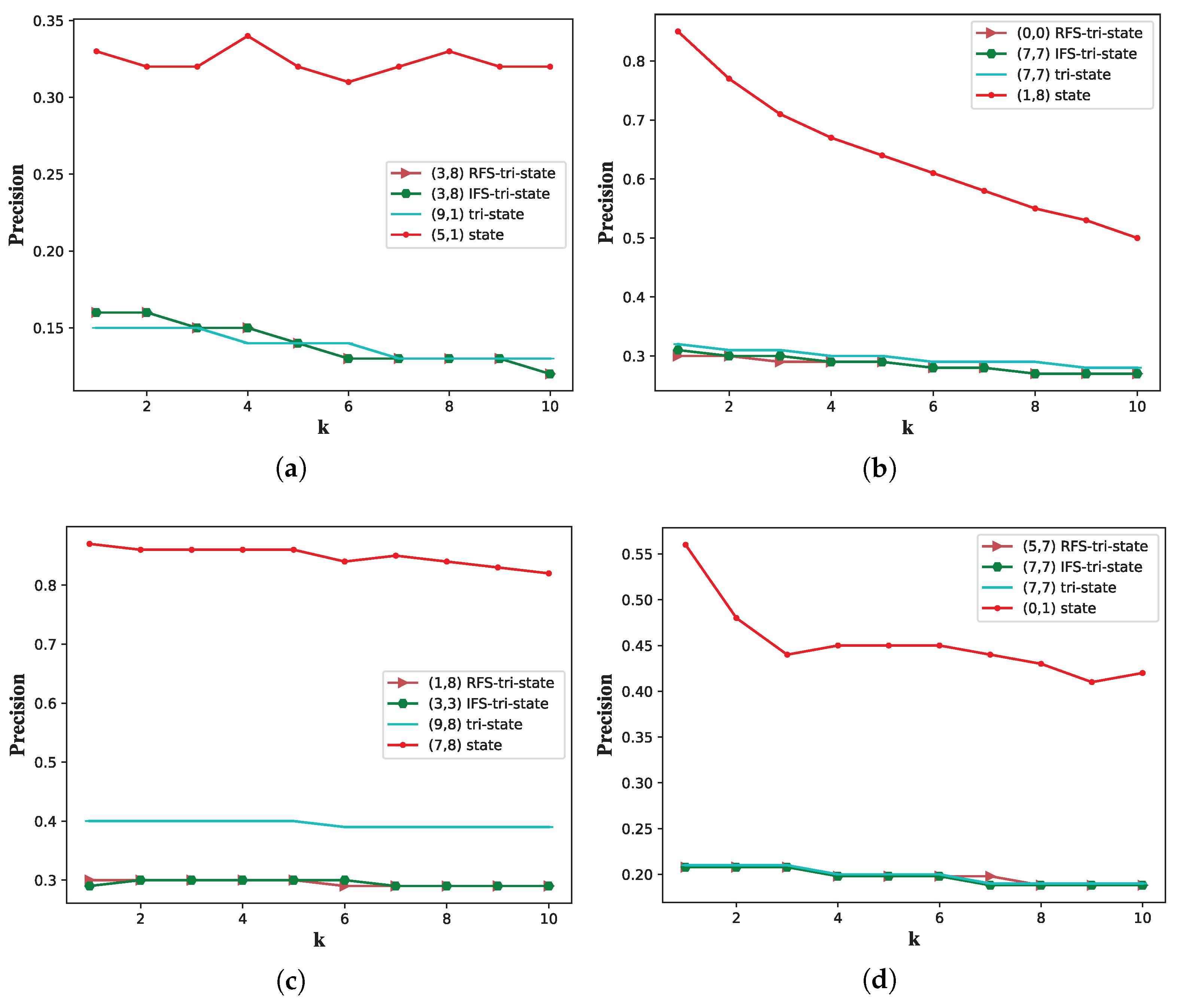
Figure 4 and Figure 5 show the meaning of precision, recall, and F1-measure for four kinds of states on the four datasets’ test sets. Commonly, the form $(r,c)$, $r,c\in [0,9]$, indicates the indices of row and column metrics, respectively. For example, $(3,8)$ means that the row metric is Levenshtein and that the column metric is Jaccard. Second, with increasing k, the precisions of the state, tri-state, IFS-based tri-state, and RFS-based state are decreased. Third, the precision of state is better than that of the others. Moreover, the precision of tri-state is slightly better than that of the IFS- and RFS-based ones. The precisions of the IFS- and RFS-based tri-states are almost consistent. This is because three kinds of tri-states provide two additional symbols for each variable. However, tri-state may be incomplete while the IFS- and RFS-based ones are complete. Therefore, the precision of the tri-state is between the state and the IFS- and RFS-based tri-states. This can be observed in Figure 4b,c.

Figure 4. The precisions of four state prediction strategies. (a) Dataset I. (b) Dataset II. (c) Dataset III. (d) Dataset IV.

Figure 5. The recalls of four state prediction strategies. (a) Dataset I. (b) Dataset II. (c) Dataset III. (d) Dataset IV.

In Figure 5, the recalls of the three kinds of tri-states are better than that of the state. Moreover, the recalls of the IFS- and RFS-based tri-states are the highest. Similarly, the recall of the tri-state is also between that of the state and the IFS- and RFS-based tri-states. Interestingly, the recall of the IFS- and RFS-based tri-states on the Stocks (Dataset II) can reach 95% and 93%, respectively.

Compared with the state, the three kinds of tri-states have better recall but worse precision. Although the improvement of IFS- and RFS-based tri-states is not significant compared to the tri-state, more information can be provided. In most cases, $k=1$ is the first choice for precision and recall.

5.3. Stability

Table 7 and Table 8 list the top 10 metric combinations for precision and recall with four kinds of states on the four datasets’ test sets. We can observe that some metric combinations are repeated. Hence, these combinations are considered more stable, with higher frequency/probability occurring in different datasets. For stronger discrimination, we additionally introduce a weighting strategy ranking for each metric combination.

Table 7. The top 10 metric combinations for precision.

Dataset	Type of State	Metric Combinations ($\mathit{r},\mathit{c}$)
I	State	(5, 1), (7, 1), (4, 1), (7, 8), (3, 7), (9, 1), (1, 8), (5, 8), (1, 7), (0, 8)
	Tri-state	(9, 1), (9, 8), (3, 8), (5, 1), (7, 8), (3, 0), (7, 1), (4, 1), (4, 7), (3, 1)
	IFS-tri-state	(3, 8), (9, 1), (9, 8), (5, 1), (3, 0), (7, 8), (8, 8), (7, 1), (4, 1), (4, 7)
	RFS-tri-state	(3, 8), (9, 1), (9, 8), (5, 1), (3, 0), (7, 8), (8, 8), (7, 1), (4, 1), (4, 7)
II	State	(1, 8), (1, 7), (5, 0), (0, 7), (0, 4), (0, 0), (7, 7), (0, 9), (1, 4), (1, 0)
	Tri-state	(7, 7), (9, 0), (8, 8), (1, 7), (8, 1), (1, 1), (1, 3), (1, 9), (1, 8), (9, 8)
	IFS-tri-state	(7, 7), (3, 0), (3, 1), (3, 7), (1, 4), (1, 0), (1, 8), (1, 9), (1, 3), (1, 1)
	RFS-tri-state	(0, 0), (3, 1), (0, 7), (5, 0), (4, 1), (5, 7), (1, 0), (1, 7), (9, 1), (1, 3)
III	State	(7, 8), (0, 8), (7, 4), (1, 4), (1, 8), (4, 8), (7, 7), (1, 7), (7, 9), (8, 8)
	Tri-state	(9, 8), (3, 3), (1, 7), (8, 8), (1, 4), (7, 8), (0, 4), (0, 8), (4, 8), (8, 0)
	IFS-tri-state	(3, 3), (7, 8), (4, 8), (9, 8), (1, 8), (0, 8), (8, 8), (9, 7), (1, 4), (0, 4)
	RFS-tri-state	(1, 8), (9, 8), (8, 1), (0, 7), (0, 1), (1, 4), (0, 8), (1, 0), (0, 4), (1, 1)
IV	State	(0, 1), (0, 7), (0, 0), (1, 0), (5, 7), (3, 7), (5, 0), (1, 1), (7, 1), (7, 0)
	Tri-state	(7, 7), (5, 7), (4, 0), (5, 0), (0, 0), (5, 1), (0, 7), (4, 7), (4, 1), (7, 0)
	IFS-tri-state	(7, 7), (5, 7), (4, 0), (5, 0), (0, 0), (5, 1), (0, 7), (4, 7), (4, 1), (7, 0)
	RFS-tri-state	(5, 7), (4, 4), (0, 7), (7, 1), (7, 8), (7, 0), (5, 1), (5, 0), (5, 4), (4, 0)

Table 8. The top 10 metric combinations for recall.

Dataset	Type of State	Metric Combinations ($\mathit{r},\mathit{c}$)
I	State	(5, 1), (7, 1), (4, 1), (7, 8), (3, 7), (9, 1), (1, 8), (5, 8), (1, 7), (0, 8)
	Tri-state	(3, 8), (9, 8), (8, 8), (4, 8), (5, 1), (5, 8), (9, 1), (3, 7), (3, 0), (5, 7)
	IFS-tri-state	(3, 8), (9, 8), (8, 8), (9, 1), (5, 1), (0, 8), (5, 8), (4, 8), (3, 7), (3, 0)
	RFS-tri-state	(3, 8), (9, 8), (8, 8), (9, 1), (5, 8), (4, 8), (0, 8), (5, 1), (3, 7), (5, 7)
II	State	(1, 8), (1, 7), (5, 0), (0, 7), (0, 4), (0, 0), (7, 7), (0, 9), (1, 4), (1, 0)
	Tri-state	(7, 7), (0, 1), (3, 1), (3, 7), (1, 4), (1, 0), (1, 8), (1, 3), (1, 1), (1, 7)
	IFS-tri-state	(0, 0), (3, 1), (0, 1), (1, 0), (1, 8), (4, 0), (7, 0), (5, 0), (0, 8), (7, 7)
	RFS-tri-state	(9, 1), (3, 1), (4, 1), (5, 1), (9, 7), (0, 8), (0, 9), (7, 7), (1, 7), (1, 0)
III	State	(7, 8), (0, 8), (7, 4), (1, 4), (1, 8), (4, 8), (7, 7), (1, 7), (7, 9), (8, 8)
	Tri-state	(9, 8), (3, 3), (1, 8), (0, 8), (4, 3), (8, 8), (7, 3), (0, 3), (1, 4), (1, 3)
	IFS-tri-state	(3, 3), (9, 8), (0, 8), (1, 4), (1, 8), (1, 3), (8, 8), (0, 4), (4, 3), (7, 3)
	RFS-tri-state	(9, 8), (1, 8), (0, 8), (1, 4), (0, 7), (1, 7), (8, 8), (0, 4), (4, 1), (1, 1)
IV	State	(0, 1), (0, 7), (0, 0), (1, 0), (5, 7), (3, 7), (5, 0), (1, 1), (7, 1), (7, 0)
	Tri-state	(7, 7), (4, 7), (0, 0), (0, 7), (7, 1), (7, 0), (0, 4), (5, 0), (5, 7), (5, 1)
	IFS-tri-state	(7, 7), (4, 7), (0, 0), (0, 7), (7, 1), (7, 0), (0, 4), (5, 0), (5, 7), (5, 1)
	RFS-tri-state	(5, 4), (7, 7), (4, 7), (0, 0), (5, 0), (0, 7), (7, 1), (7, 0), (4, 1), (7, 4)

Given a metric combination $x\in [0,9]$:

$$\rho \left(x\right)=\frac{\xi \left(x\right)}{2^{\pi \left(x\right)}}$$

(24)

is the stability metric of x. Among them, $\xi \left(x\right)$ is the occurrence on four datasets. Moreover:

$$\pi \left(x\right)=\frac{{\Sigma }_{i\in \left\{\mathrm{I},\mathrm{II},\mathrm{III},\mathrm{IV}\right\}}\eta (x,i)}{\xi \left(x\right)}$$

(25)

is the average ranking of x. If x does not occur in dataset i, $\eta (x,i)=0$. Otherwise, $\eta (x,i)$ is the ranking of x.

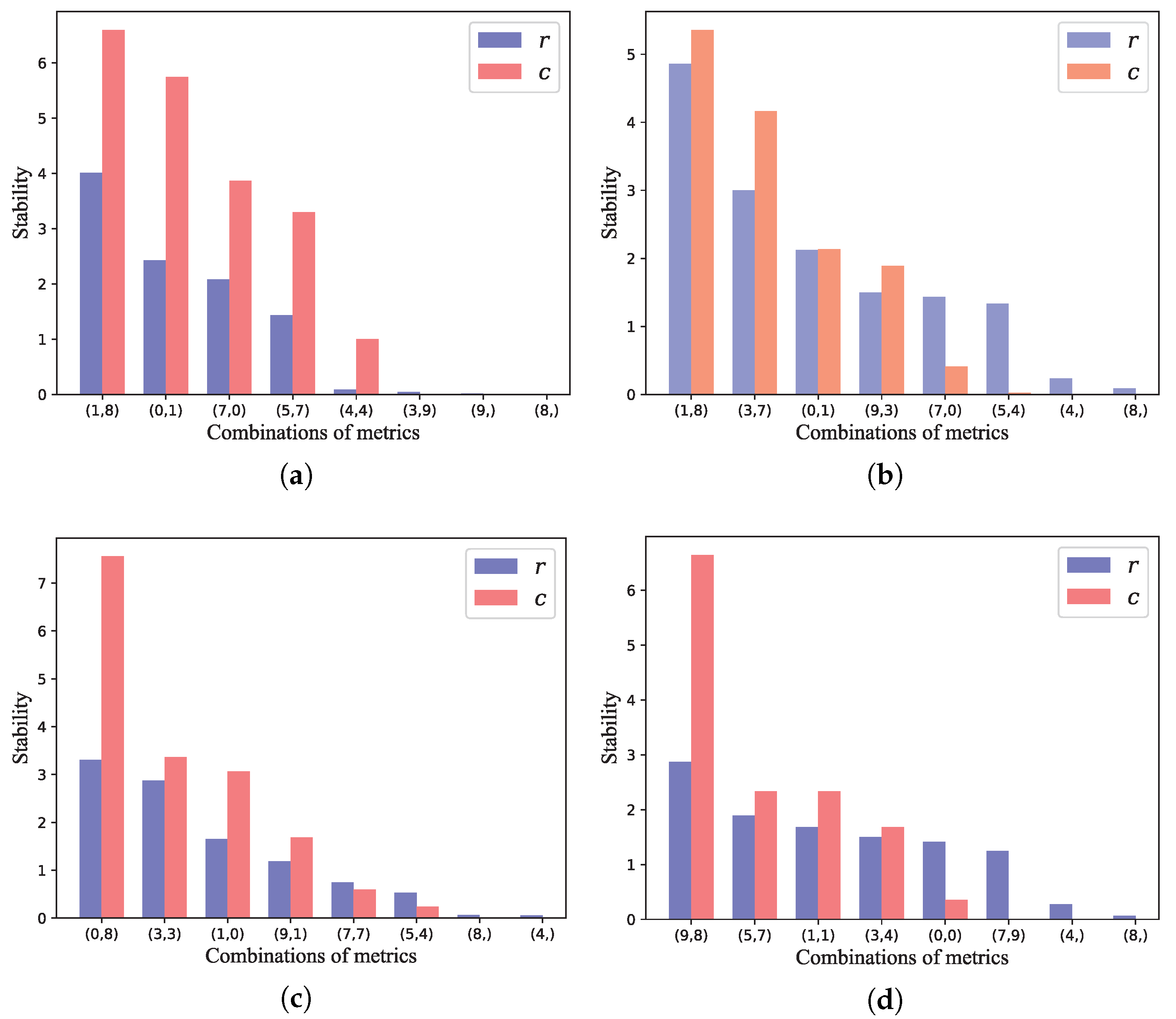
Figure 6 shows the most stable metric combinations for precision. In terms of the state, combination $(1,8)$ is the first choice. In terms of the tri-state, combination $(1,8)$ is the first choice. In terms of the IFS-based tri-state, combination $(3,8)$ is the first choice. In terms of the RFS-based tri-state, combination $(3,8)$ is the first choice.

Figure 6. The most stable metric combinations for precision. (a) State. (b) Tri-state. (c) IFS-tri-state. (d) RFS-tri-state.

Figure 7 shows the most stable metric combinations for recall. In terms of the state, combination $(1,8)$ is the first choice. In terms of the tri-state, combination $(1,8)$ is the first choice. In terms of the IFS-based tri-state, combination $(0,8)$ is the first choice. In terms of the RFS-based tri-state, combination $(9,8)$ is the first choice.

Figure 7. The most stable metric combinations for recall. (a) State. (b) Tri-state. (c) IFS-tri-state. (d) RFS-tri-state.

With the above observations, the eighth metric, i.e., the Jaccard similarity, is the most frequently used, followed by the second one, i.e., the Manhattan distance.

6. Conclusions

In this paper, a new tri-state and its prediction problem were defined on multivariate time-series (MTS). The most likely occurring strong, medium, and weak symbols can be obtained with the tri-state. Second, a deviation degree-based tri-partition strategy and the algorithm were designed. For all symbols of each variable, the symbol was stronger and deviated further from the average value. Third, the along–across similarity model was proposed to capture the temporal and variables’ association relationships. Fourth, the integration of the PAA and SAX versions of MTS can combine numerical or symbolic similarities or distances. Finally, when a new dataset is introduced, the first choices in parameter settings are $k=1$ (the size neighborhood), $r=1$ (the Jaccard), and $c=8$ (the Manhattan).

The following research topics deserve further investigation:

• More alphabet tri-partition strategies;
• More tri-state completion strategies;
• Adaptive learning of the parameters by cost-sensitive learning; and
• More intelligent metrics combination strategies, e.g., integrated learning.

References

- Wei, W.W.S. Multivariate Time Series Analysis and Applications; John Wiley & Sons: Hoboken, NJ, USA, 2018. [Google Scholar]
- Park, H.; Jung, J.Y. SAX-ARM: Deviant event pattern discovery from multivariate time series using symbolic aggregate approximation and association rule mining. Expert Syst. Appl. 2020, 141, 112950. [Google Scholar] [CrossRef]
- Xu, J.; Tang, L.; Zeng, C.; Li, T. Pattern discovery via constraint programming. Knowl.-Based Syst. 2016, 94, 23–32. [Google Scholar] [CrossRef]
- Zhang, Z.H.; Min, F. Frequent state transition patterns of multivariate time series. IEEE Access 2019, 7, 142934–142946. [Google Scholar] [CrossRef]
- Zhang, Z.H.; Min, F.; Chen, G.S.; Shen, S.P.; Wen, Z.C.; Zhou, X.B. Tri-Partition state alphabet-based sequential pattern for multivariate time series. Cogn. Comput. 2021, 1–19. [Google Scholar] [CrossRef]
- Cheng, R.; Hu, H.; Tan, X.; Bai, Y. Initialization by a novel clustering for wavelet neural network as time series predictor. Comput. Intell. Neurosci. 2015, 2015, 1–9. [Google Scholar] [CrossRef] [PubMed]
- Li, H.L. Multivariate time series clustering based on common principal component analysis. Neurocomputing 2019, 349, 239–247. [Google Scholar] [CrossRef]
- Li, H.L.; Liu, Z.C. Multivariate time series clustering based on complex network. Pattern Recognit. 2021, 115, 107919. [Google Scholar] [CrossRef]
- Baldán, F.J.; Benítez, J.M. Multivariate times series classification through an interpretable representation. Inf. Sci. 2021, 569, 596–614. [Google Scholar] [CrossRef]
- Baydogan, M.G.; Runger, G. Learning a symbolic representation for multivariate time series classification. Data Min. Knowl. Discov. 2015, 29, 400–422. [Google Scholar] [CrossRef]
- Araújo, R.D.A. A class of hybrid morphological perceptrons with application in time series forecasting. Knowl.-Based Syst. 2011, 24, 513–529. [Google Scholar] [CrossRef]
- Sugihara, G.; May, R.; Ye, H.; Hsieh, C.H.; Deyle, E.; Fogarty, M.; Munch, S. Detecting Causality in Complex Ecosystems. Science 2012, 338, 496–500. [Google Scholar] [CrossRef] [PubMed]
- Ren, H.R.; Liu, M.M.; Li, Z.W.; Pedrycz, W. A piecewise aggregate pattern representation approach for anomaly detection in time series. Knowl.-Based Syst. 2017, 135, 29–39. [Google Scholar] [CrossRef]
- Ju, Y.; Sun, G.Y.; Chen, Q.H.; Zhang, M.; Zhu, H.X.; Rehman, M.U. A model combining convolutional neural network and LightGBM algorithm for ultra-short-term wind power forecasting. IEEE Access 2019, 7, 28309–28318. [Google Scholar] [CrossRef]
- Zhang, N.; Lin, A.; Shang, P. Multidimensional k-nearest neighbor model based on EEMD for financial time series forecasting. Phys. A Stat. Mech. Appl. 2017, 477, 161–173. [Google Scholar] [CrossRef]
- Shen, F.; Liu, J.; Wu, K. Multivariate Time Series Forecasting based on Elastic Net and High-Order Fuzzy Cognitive Maps: A Case Study on Human Action Prediction through EEG Signals. IEEE Trans. Fuzzy Syst. 2020, 29, 2336–2348. [Google Scholar] [CrossRef]
- Xu, D.W.; Wang, Y.D.; Peng, P.; Shen, B.L.; Deng, Z.; Guo, H.F. Real-time road traffic state prediction based on kernel-kNN. Transp. A Transp. Sci. 2020, 16, 104–118. [Google Scholar] [CrossRef]
- Yin, Y.; Shang, P.J. Forecasting traffic time series with multivariate predicting method. Appl. Math. Comput. 2016, 291, 266–278. [Google Scholar] [CrossRef]
- Ma, J.; Cheng, J.C.; Lin, C.Q.; Tan, Y.; Zhang, J.C. Improving air quality prediction accuracy at larger temporal resolutions using deep learning and transfer learning techniques. Atmos. Environ. 2019, 214, 116885. [Google Scholar] [CrossRef]
- Liu, P.H.; Liu, J.; Wu, K. CNN-FCM: System modeling promotes stability of deep learning in time series prediction. Knowl.-Based Syst. 2020, 203, 106081. [Google Scholar] [CrossRef]
- Martínez, F.; Frías, M.P.; Pérez, M.D.; Rivera, A.J. A methodology for applying k-nearest neighbor to time series forecasting. Artif. Intell. Rev. 2019, 52, 2019–2037. [Google Scholar] [CrossRef]
- Weytjens, H.; Lohmann, E.; Kleinsteuber, M. Cash flow prediction: MLP and LSTM compared to ARIMA and Prophet. Electron. Commer. Res. 2021, 21, 371–391. [Google Scholar] [CrossRef]
- Zhou, Y.; Cheung, Y.M. Bayesian low-tubal-rank robust tensor factorization with multi-rank determination. IEEE Trans. Pattern Anal. Mach. Intell. 2019, 43, 62–76. [Google Scholar] [CrossRef]
- Zhou, Y.; Lu, H.; Cheung, Y.M. Probabilistic rank-one tensor analysis with concurrent regularizations. IEEE Trans. Cybern. 2021, 51, 3496–3509. [Google Scholar] [CrossRef]
- Chen, T.T.; Lee, S.J. A weighted LS-SVM based learning system for time series forecasting. Inf. Sci. 2015, 299, 99–116. [Google Scholar] [CrossRef]
- Jimenez, F.; Palma, J.; Sanchez, G.; Marin, D.; Palacios, M.F.; López, M.L. Feature selection based multivariate time series forecasting: An application to antibiotic resistance outbreaks prediction. Artif. Intell. Med. 2020, 104, 101818. [Google Scholar] [CrossRef]
- Qiu, X.H.; Zhang, L.; Suganthan, P.N.; Amaratunga, G.A.J. Oblique random forest ensemble via least square estimation for time series forecasting. Inf. Sci. 2017, 420, 249–262. [Google Scholar] [CrossRef]
- Yao, Y.Y. The geometry of three-way decision. Appl. Intell. 2021, 51, 6298–6325. [Google Scholar] [CrossRef]
- Yao, Y.Y. Set-theoretic models of three-way decision. Granul. Comput. 2021, 6, 133–148. [Google Scholar] [CrossRef]
- Yao, Y.Y. Tri-level thinking: Models of three-way decision. Int. J. Mach. Learn. Cybern. 2020, 11, 947–959. [Google Scholar] [CrossRef]
- Sang, B.B.; Guo, Y.T.; Shi, D.R.; Xu, W.H. Decision-theoretic rough set model of multi-source decision systems. Int. J. Mach. Learn. Cybern. 2018, 9, 1941–1954. [Google Scholar] [CrossRef]
- Li, J.H.; Huang, C.C.; Qi, J.J.; Qian, Y.H.; Liu, W.Q. Three-way cognitive concept learning via multi-granularity. Inf. Sci. 2017, 378, 244–263. [Google Scholar] [CrossRef]
- Yao, Y.Y. Three-way decisions and cognitive computing. Cogn. Comput. 2016, 8, 543–554. [Google Scholar] [CrossRef]
- Deng, X.F.; Yao, Y.Y. Decision-theoretic three-way approximations of fuzzy sets. Inf. Sci. 2014, 279, 702–715. [Google Scholar] [CrossRef]
- Hu, B.Q. Three-way decisions space and three-way decisions. Inf. Sci. 2014, 281, 21–52. [Google Scholar] [CrossRef]
- Qian, J.; Liu, C.H.; Miao, D.Q.; Yue, X.D. Sequential three-way decisions via multi-granularity. Inf. Sci. 2020, 507, 606–629. [Google Scholar] [CrossRef]
- Li, X.N.; Yi, H.J.; She, Y.H.; Sun, B.Z. Generalized three-way decision models based on subset evaluation. Int. J. Approx. Reason. 2017, 83, 142–159. [Google Scholar] [CrossRef]
- Liu, D.; Liang, D.C.; Wang, C.C. A novel three-way decision model based on incomplete information system. Knowl.-Based Syst. 2016, 91, 32–45. [Google Scholar] [CrossRef]
- Xu, W.H.; Li, M.M.; Wang, X.Z. Information Fusion Based on Information Entropy in Fuzzy Multi-source Incomplete Information System. Int. J. Fuzzy Syst. 2017, 19, 1200–1216. [Google Scholar] [CrossRef]
- Zhang, H.R.; Min, F.; Shi, B. Regression-based three-way recommendation. Inf. Sci. 2017, 378, 444–461. [Google Scholar] [CrossRef]
- Wang, M.; Min, F.; Zhang, Z.H.; Wu, Y.X. Active learning through density clustering. Expert Syst. Appl. 2017, 85, 305–317. [Google Scholar] [CrossRef]
- Yu, H.; Wang, X.C.; Wang, G.Y.; Zeng, X.H. An active three-way clustering method via low-rank matrices for multi-view data. Inf. Sci. 2020, 507, 823–839. [Google Scholar] [CrossRef]
- Yue, X.D.; Chen, Y.F.; Miao, D.Q.; Qian, J. Tri-partition neighborhood covering reduction for robust classification. Int. J. Approx. Reason. 2016, 83, 371–384. [Google Scholar] [CrossRef]
- Zhou, B.; Yao, Y.Y.; Luo, J.G. Cost-sensitive three-way email spam filtering. J. Intell. Inf. Syst. 2014, 42, 19–45. [Google Scholar] [CrossRef]
- Li, H.X.; Zhang, L.B.; Huang, B.; Zhou, X.Z. Sequential three-way decision and granulation for cost-sensitive face recognition. Knowl.-Based Syst. 2016, 91, 241–251. [Google Scholar] [CrossRef]
- Min, F.; Zhang, Z.H.; Zhai, W.J.; Shen, R.P. Frequent pattern discovery with tri-partition alphabets. Inf. Sci. 2020, 507, 715–732. [Google Scholar] [CrossRef]
- Lin, J.; Keogh, E.; Wei, L.; Lonardi, S. Experiencing SAX: A novel symbolic representation of time series. Data Min. Knowl. Discov. 2007, 15, 107–144. [Google Scholar] [CrossRef]
- Shi, Q.Q.; Yin, J.M.; Cai, J.J.; Cichocki, A.; Yokota, T.; Chen, L.; Yuan, M.X.; Zeng, J. Block Hankel tensor ARIMA for multiple short time series forecasting. In Proceedings of the AAAI Conference on Artificial Intelligence, New York, NY, USA, 7–12 February 2020; Volumr 34, pp. 5758–5766. [Google Scholar]
- Ma, X.Y.; Zhang, L.; Xu, L.; Liu, Z.C.; Chen, G.; Xiao, Z.L.; Wang, Y.; Wu, Z.T. Large-scale user visits understanding and forecasting with deep spatial-temporal tensor factorization framework. In Proceedings of the 25th ACM SIGKDD International Conference on Knowledge Discovery & Data Mining, Anchorage, AK, USA, 4–8 August 2019; pp. 2403–2411. [Google Scholar]
- Chen, X.Y.; Sun, L.J. Low-rank autoregressive tensor completion for multivariate time series forecasting. arXiv 2020, arXiv:2006.10436. [Google Scholar]
- Wu, Y.K.; Zhuang, D.Y.; Labbe, A.; Sun, L.J. Inductive graph neural networks for spatiotemporal kriging. arXiv 2020, arXiv:2006.07527. [Google Scholar]
- Lonardi, S.; Lin, J.; Keogh, E.; Chiu, B.Y.C. Efficient discovery of unusual patterns in time series. New Gener. Comput. 2006, 25, 61–93. [Google Scholar] [CrossRef][Green Version]
- Amir, A.; Charalampopoulos, P.; Pissis, S.P.; Radoszewski, J. Dynamic and internal longest common substring. Algorithmica 2020, 82, 3707–3743. [Google Scholar] [CrossRef]
- Behara, K.N.; Bhaskar, A.; Chung, E. A novel approach for the structural comparison of origin-destination matrices: Levenshtein distance. Transp. Res. Part C Emerg. Technol. 2020, 111, 513–530. [Google Scholar] [CrossRef]
- Chung, N.C.; Miasojedow, B.; Startek, M.; Gambin, A. Jaccard/Tanimoto similarity test and estimation methods for biological presence-absence data. BMC Bioinform. 2019, 20, 644. [Google Scholar] [CrossRef] [PubMed]
- Sun, S.B.; Zhang, Z.H.; Dong, X.L.; Zhang, H.R.; Li, T.J.; Zhang, L.; Min, F. Integrating triangle and jaccard similarities for recommendation. PLoS ONE 2017, 12, e0183570. [Google Scholar] [CrossRef] [PubMed]
Publisher’s Note: MDPI stays neutral with regard to jurisdictional claims in published maps and institutional affiliations. |
© 2021 by the authors. Licensee MDPI, Basel, Switzerland. This article is an open access article distributed under the terms and conditions of the Creative Commons Attribution (CC BY) license (https://creativecommons.org/licenses/by/4.0/).