
Long Distance Moving Vehicle Tracking with a Multirotor Based on IMM-Directional Track Association


Abstract
:1. Introduction
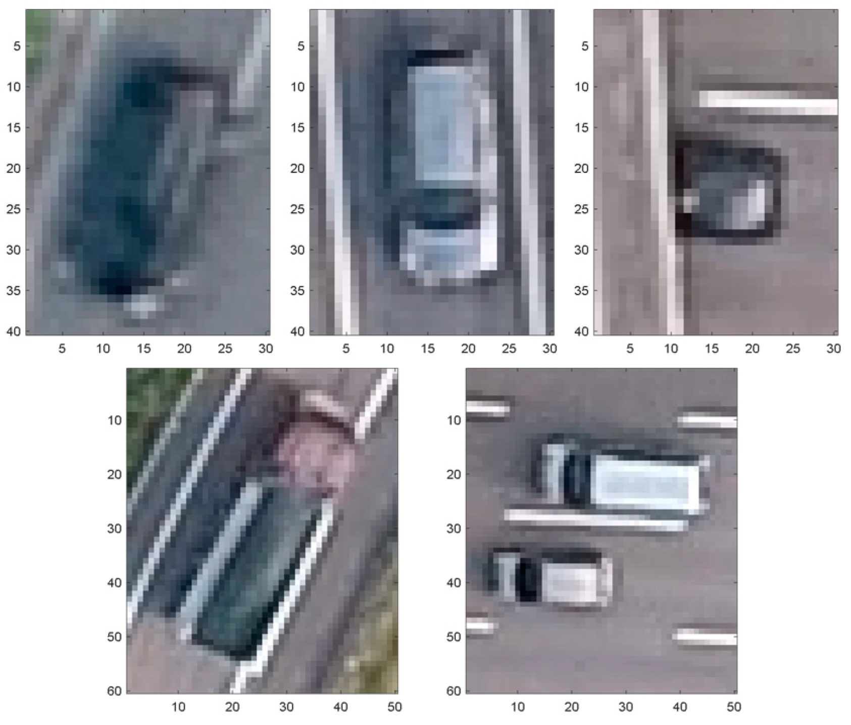
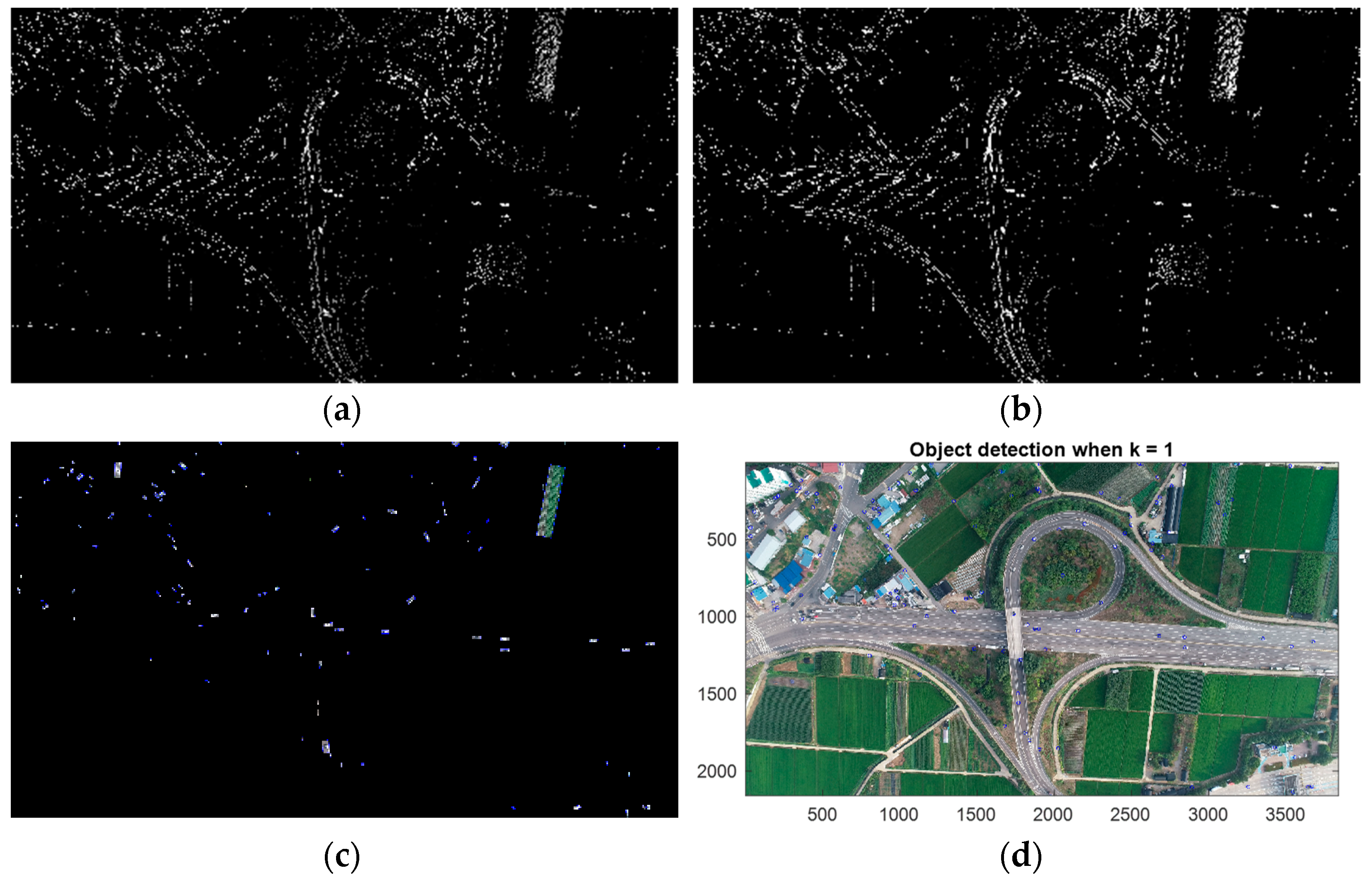
2. Moving Object Detection
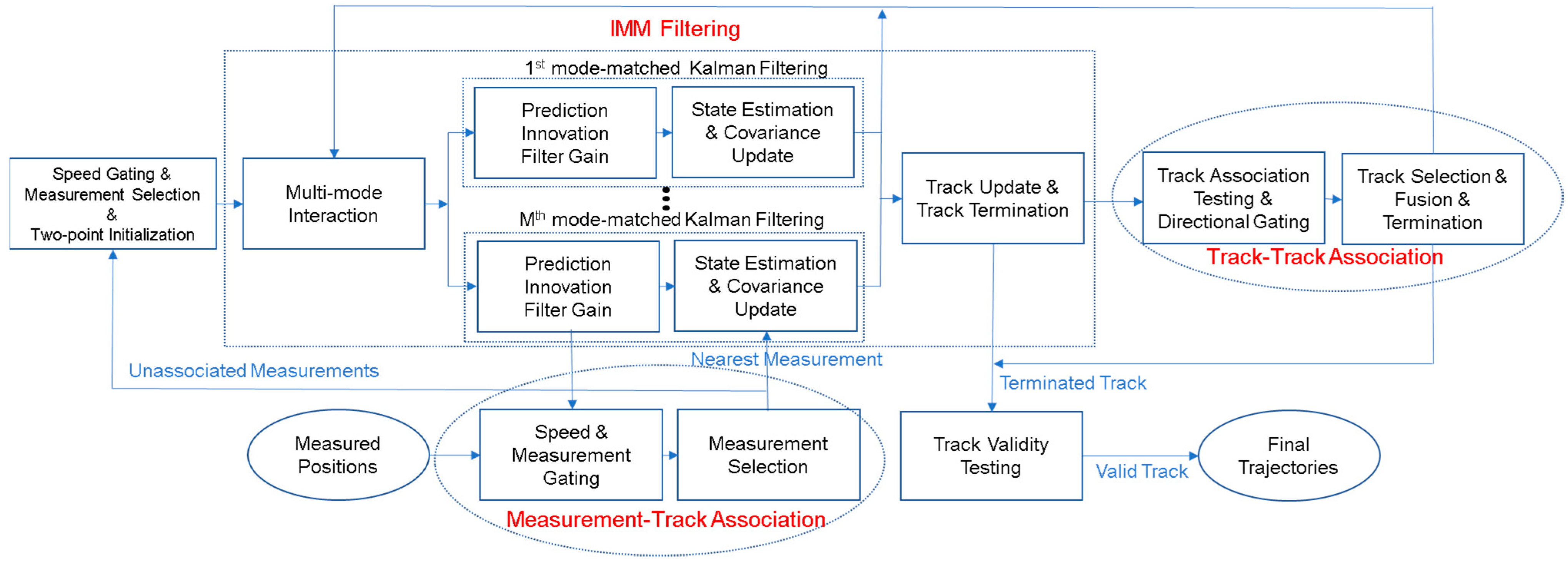
3. Multiple Target Tracking
3.1. System Modeling
3.2. Two Point Differencing Intialization
3.3. Multi-Mode Interaction
3.4. Mode Matched Kalman Filtering
3.5. Measurement-to-Track Association
3.6. Mode State Estimate and Covariance Update
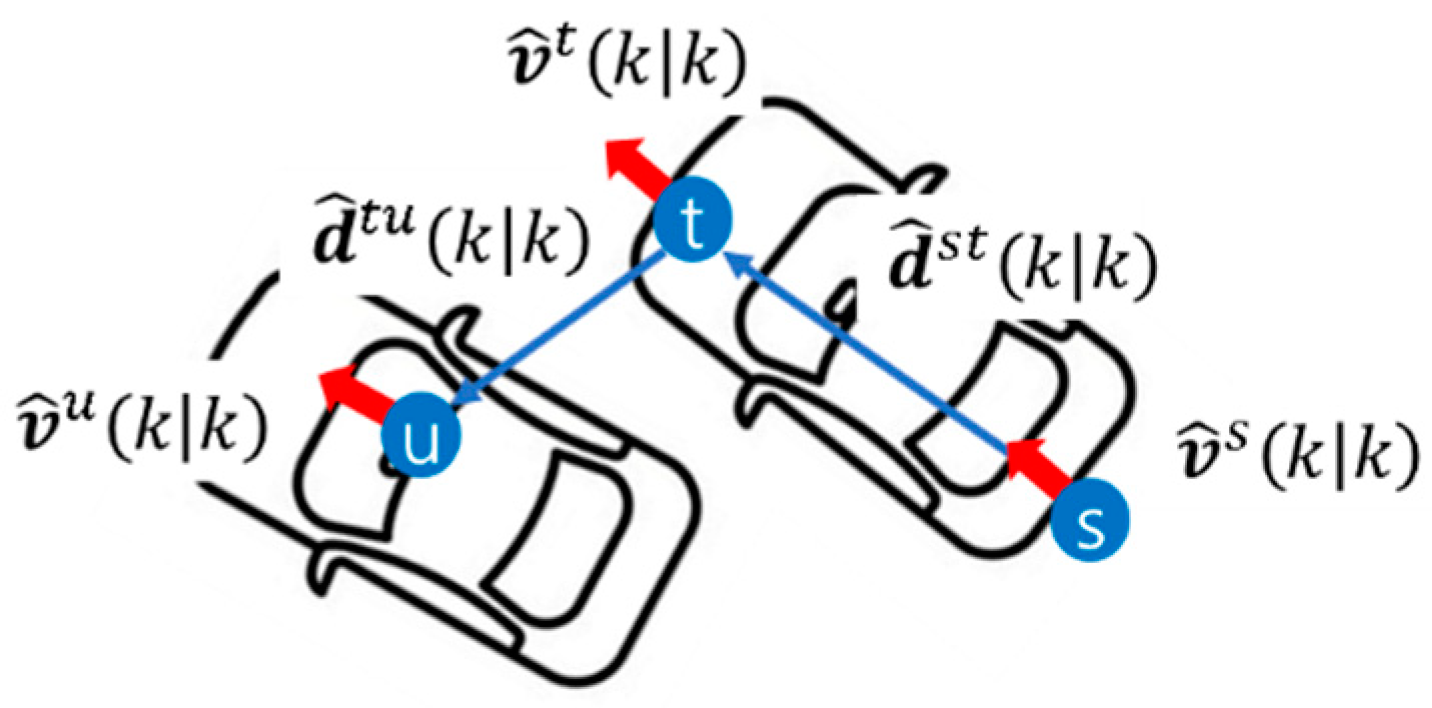
3.7. Directional Track-to-Track Association
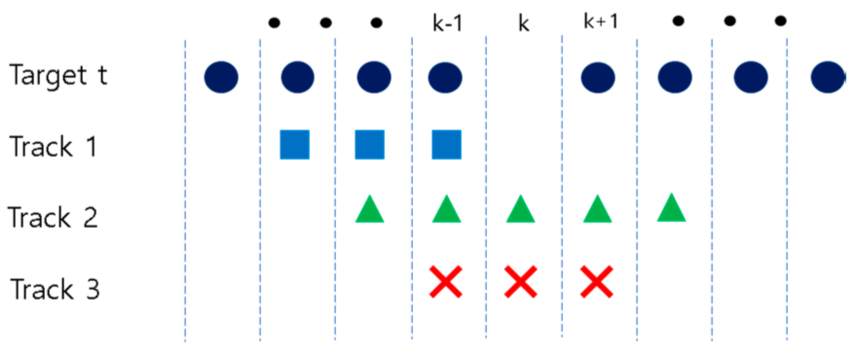
3.8. Track Termination and Validity Testing
4. Results
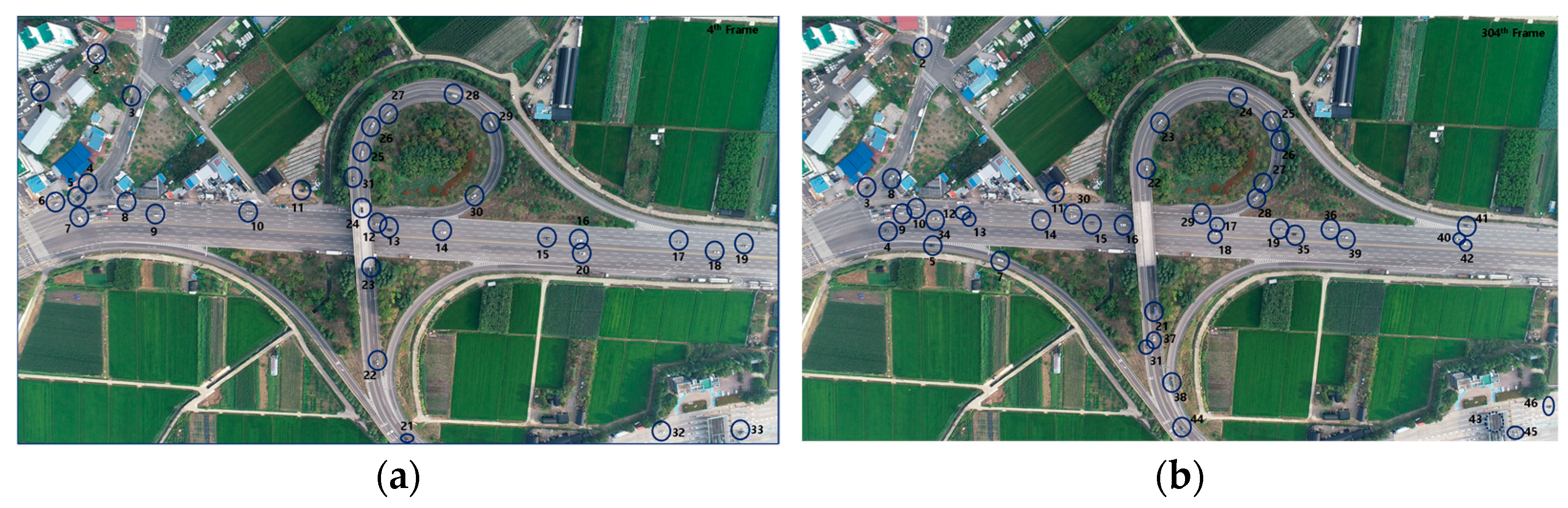
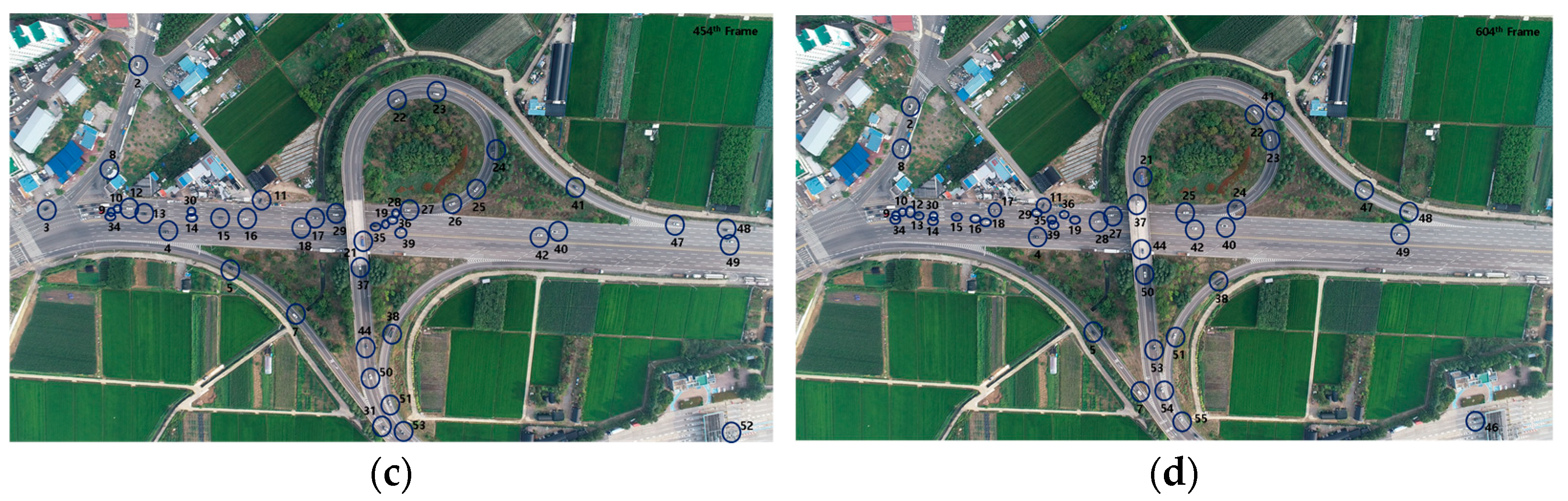
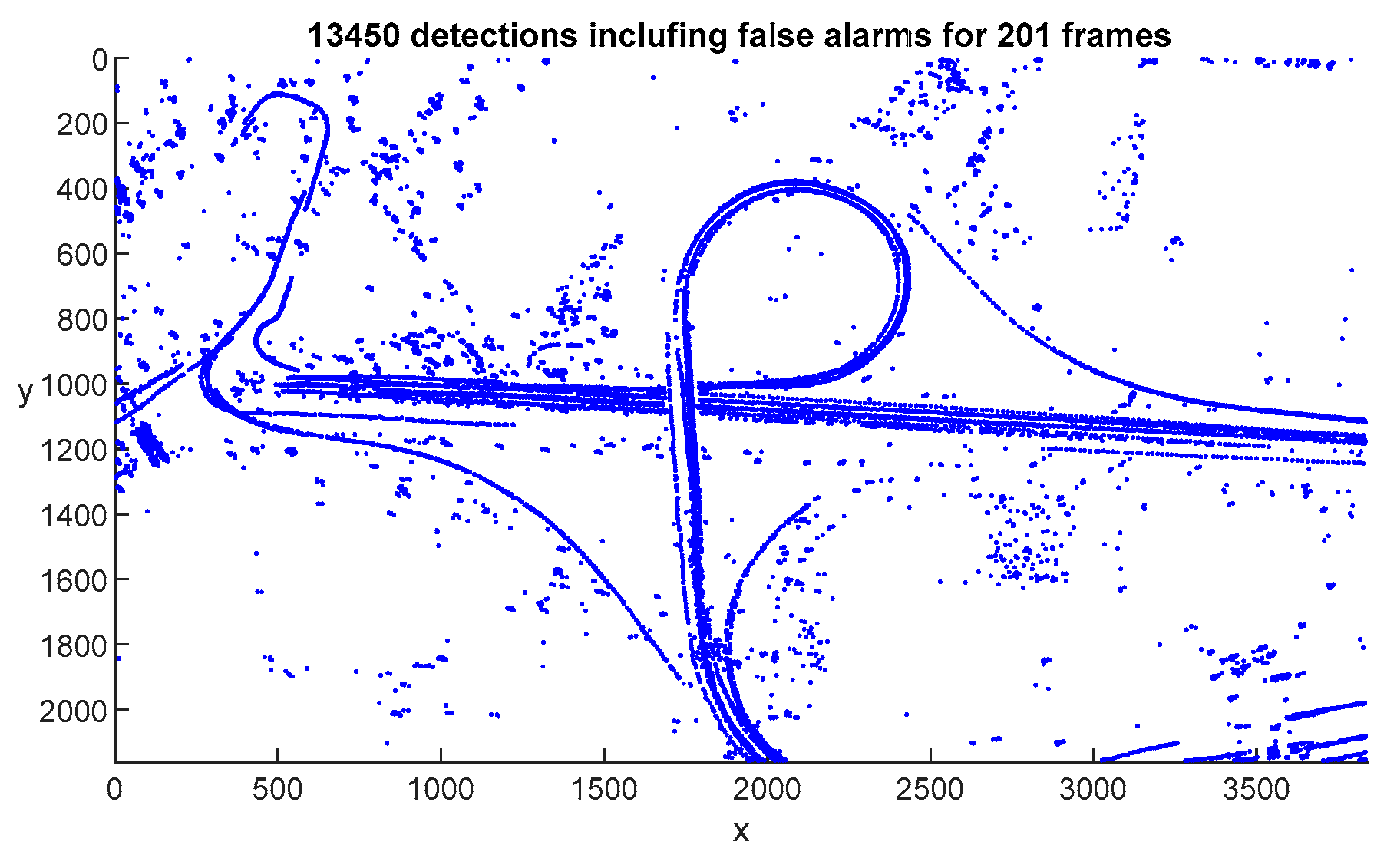
4.1. Video Description and Moving Object Detection
4.2. Multiple Target Tracking
5. Discussion
6. Conclusions
Supplementary Materials
Funding
Institutional Review Board Statement
Informed Consent Statement
Data Availability Statement
Acknowledgments
Conflicts of Interest
References
- Alzahrani, B.; Oubbati, O.S.; Barnawi, A.; Atiquzzaman, M.; Alghazzawi, D. UAV assistance paradigm: State-of-the-art in applications and challenges. J. Netw. Comput. Appl. 2020, 166, 102706. [Google Scholar] [CrossRef]
- Zaheer, Z.; Usmani, A.; Khan, E.; Qadeer, M.A. Aerial surveillance system using UAV. In Proceedings of the 2016 Thirteenth International Conference on Wireless and Optical Communications Networks (WOCN), Hyderabad, India, 21–23 July 2016; pp. 1–7. [Google Scholar]
- Theys, B.; Schutter, J.D. Forward flight tests of a quadcopter unmanned aerial vehicle with various spherical body diameters. Int. J. Micro Air Veh. 2020, 12, 1–8. [Google Scholar] [CrossRef]
- Li, S.; Yeung, D.-Y. Visual object tracking for unmanned aerial vehicles: A benchmark and new motion models. In Proceeding of the Thirty-Frist AAAI conference on Artificial Intelligence (AAAI-17), San Francisco, CA, USA, 4–9 February 2017; pp. 4140–4146. [Google Scholar]
- Du, D.; Qi, Y.; Yu, H.; Yang, Y.; Duan, K.; Li, G.; Zhang, W.; Huang, Q.; Tian, Q. The Unmanned Aerial Vehicle Benchmark: Object Detection and Tracking. In Computer Vision—ECCV 2018; Lecture Notes in Computer Science; Springer: Cham, Switzerland, 2018; pp. 375–391. [Google Scholar] [CrossRef] [Green Version]
- Zhang, H.; Lei, Z.; Wang, G.; Hwang, J. Eye in the Sky: Drone-Based Object Tracking and 3D Localization. In Proceedings of the 27th ACM International Conference on Multimedia, Nice, France, 21–25 October 2019; pp. 899–907. [Google Scholar] [CrossRef] [Green Version]
- Zhang, S.; Zhuo, L.; Zhang, H.; Li, J. Object Tracking in Unmanned Aerial Vehicle Videos via Multifeature Discrimination and Instance-Aware Attention Network. Remote Sens. 2020, 12, 2646. [Google Scholar] [CrossRef]
- Kouris, A.; Kyrkou, C.; Bouganis, C.-S. Informed Region Selection for Efficient UAV-Based Object Detectors: Altitude-Aware Vehicle Detection with Cycar Dataset. In Proceedings of the IEEE/RSJ International Conference on Intelligent Robots and Systems (IROS), Macau, China, 4–9 November 2019; pp. 51–58. [Google Scholar]
- Kamate, S.; Yilmazer, N. Application of Object Detection and Tracking Techniques for Unmanned Aerial Vehicles. Procedia Comput. Sci. 2015, 61, 436–441. [Google Scholar] [CrossRef] [Green Version]
- Fang, P.; Lu, J.; Tian, Y.; Miao, Z. An Improved Object Tracking Method in UAV Videos. Procedia Eng. 2011, 15, 634–638. [Google Scholar] [CrossRef]
- Jianfang, L.; Hao, Z.; Jingli, G. A novel fast target tracking method for UAV aerial image. Open Physics 2017, 15, 420–426. [Google Scholar] [CrossRef] [Green Version]
- Sinha, A.; Kirubarajan, T.; Bar-Shalom, Y. Autonomous Ground Target Tracking by Multiple Cooperative UAVs. In Proceedings of the 2005 IEEE Aerospace Conference, Big Sky, MT, USA, 5–12 March 2005; pp. 1–9. [Google Scholar]
- Guido, G.; Gallelli, V.; Rogano, D.; Vitale, A. Evaluating the accuracy of vehicle tracking data obtained from Unmanned Aerial Vehicles. Int. J. Transp. Sci. Technol. 2016, 5, 136–151. [Google Scholar] [CrossRef]
- Rajasekaran, R.K.; Ahmed, N.; Frew, E. Bayesian Fusion of Unlabeled Vision and RF Data for Aerial Tracking of Ground Targets. In Proceedings of the IEEE/RSJ International Conference on Intelligent Robots and Systems (IROS), Las Vegas, NV, USA, 24 October 2020–24 January 2021; pp. 1629–1636. [Google Scholar]
- Stone, L.D.; Streit, R.L.; Corwin, T.L.; Bell, K.L. Bayesian Multiple Target Tracking, 2nd ed.; Artech House: Boston, MA, USA, 2014. [Google Scholar]
- Blom, H.A.P.; Bar-shalom, Y. The interacting multiple model algorithm for systems with Markovian switching coefficients. IEEE Trans. Autom. Control 1988, 33, 780–783. [Google Scholar] [CrossRef]
- Bar-Shalom, Y.; Fortmann, T.E. Tracking and Data Association; Academic Press Inc.: Orlando, FL, USA, 1989. [Google Scholar]
- Bar-Shalom, Y.; Li, X.R. Multitarget-Multisensor Tracking: Principles and Techniques; YBS Publishing: Storrs, CT, USA, 1995. [Google Scholar]
- Lee, M.-H.; Yeom, S. Multiple target detection and tracking on urban roads with a drone. J. Intell. Fuzzy Syst. 2018, 35, 6071–6078. [Google Scholar] [CrossRef]
- Yeom, S.; Cho, I.-J. Detection and Tracking of Moving Pedestrians with a Small Unmanned Aerial Vehicle. Appl. Sci. 2019, 9, 3359. [Google Scholar] [CrossRef] [Green Version]
- Yeom, S.; Nam, D.-H. Moving Vehicle Tracking with a Moving Drone Based on Track Association. Appl. Sci. 2021, 11, 4046. [Google Scholar] [CrossRef]
- Yeom, S. Moving People Tracking and False Track Removing with Infrared Thermal Imaging by a Multirotor. Drones 2021, 5, 65. [Google Scholar] [CrossRef]
- Houles, A.; Bar-Shalom, Y. Multisensor Tracking of a Maneuvering Target in Clutter. IEEE Trans. Aerosp. Electron. Syst. 1989, 25, 176–189. [Google Scholar] [CrossRef]
- Peng, Z.; Li, F.; Liu, J.; Ju, Z. A Symplectic Instantaneous Optimal Control for Robot Trajectory Tracking with Differential-Algebraic Equation Models. IEEE Trans. Ind. Electron. 2020, 67, 3819–3829. [Google Scholar] [CrossRef] [Green Version]
- Li, X.R.; Jilkov, V.P. Survey of maneuvering target tracking, part I: Dynamic models. IEEE Trans. Aerosp. Electron. Syst. 2003, 39, 1333–1364. [Google Scholar]
- Moore, J.R.; Blair, W.D. Multitarget-Multisensor Tracking: Applications and Advances; Bar-Shalom, Y., Blair, W.D., Eds.; Practical Aspects of Multisensor Tracking, Chap. 1; Artech House: Boston, MA, USA, 2000; Volume III. [Google Scholar]
- Yeom, S.-W.; Kirubarajan, T.; Bar-Shalom, Y. Track segment association, fine-step IMM and initialization with doppler for improved track performance. IEEE Trans. Aerosp. Electron. Syst. 2004, 40, 293–309. [Google Scholar] [CrossRef]


| Parameters | IMM-CV | IMM-CA | |
|---|---|---|---|
| Sampling time | 0.1 s | ||
| Max. target speed for initialization, Vmax | 30 m/s | ||
| Process noise variance | 1 m/s2 | 0.01 m/s2 | |
| 10 m/s2 | 0.1 m/s2 | ||
| Mode transition probabiltiy pij | |||
| Measurement noise variance, | 1.5 m | ||
| Measurent association | Gate threshold, | 8 | |
| Max. target speed, Smax | 35 m/s | ||
| Track association | Gate threshold, | 70 | |
| Angle threhold, | |||
| Track termination | Max. searching number | 20 frames (=2 s) | |
| Min. target speed | 1 m/s | ||
| Min. track life length for track validity | 20 frames (=2 s) | ||
| IMM-CV | IMM-CA | |||
|---|---|---|---|---|
| Track Association | Directional TA | Track Association | Directional TA | |
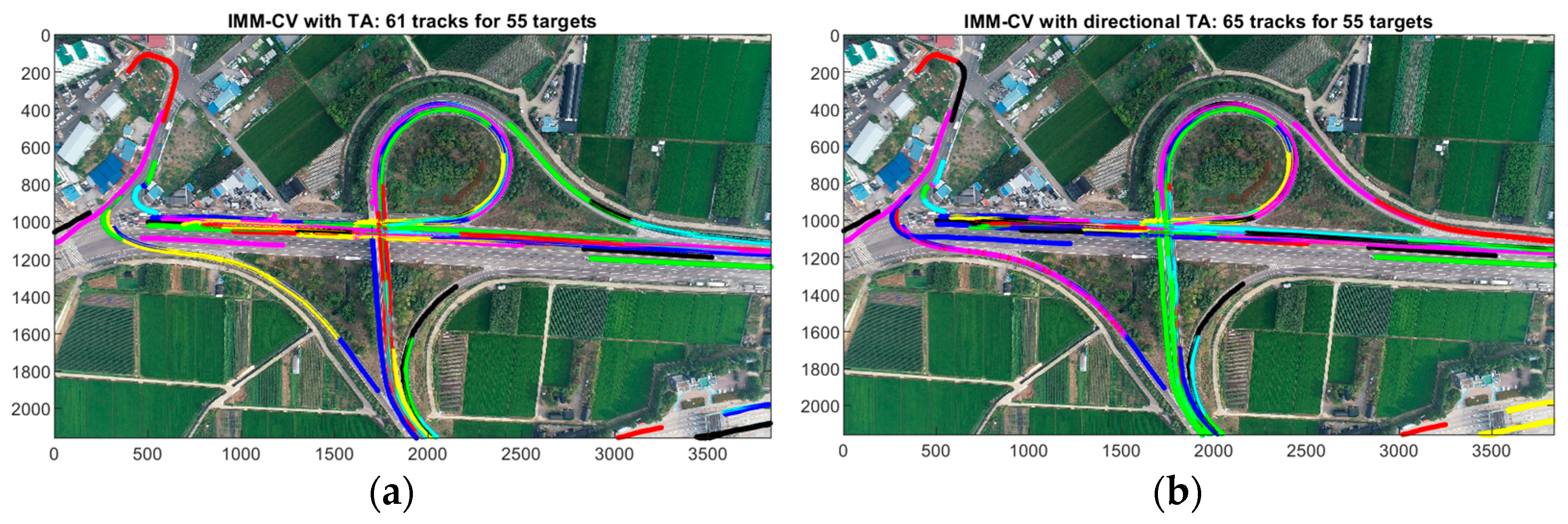
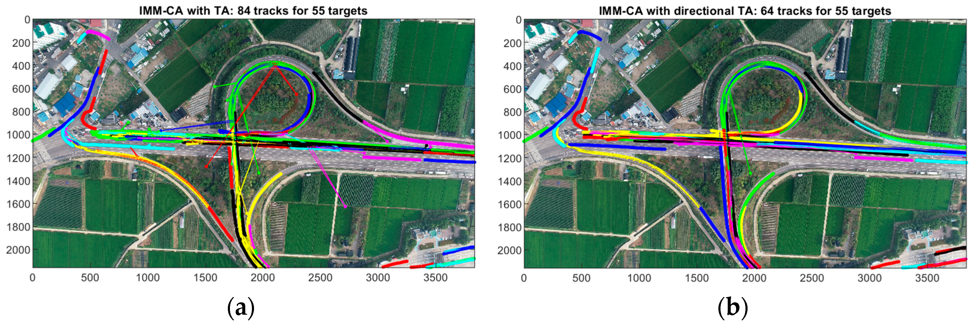
| Number of tracks | 61 | 65 | 84 | 64 |
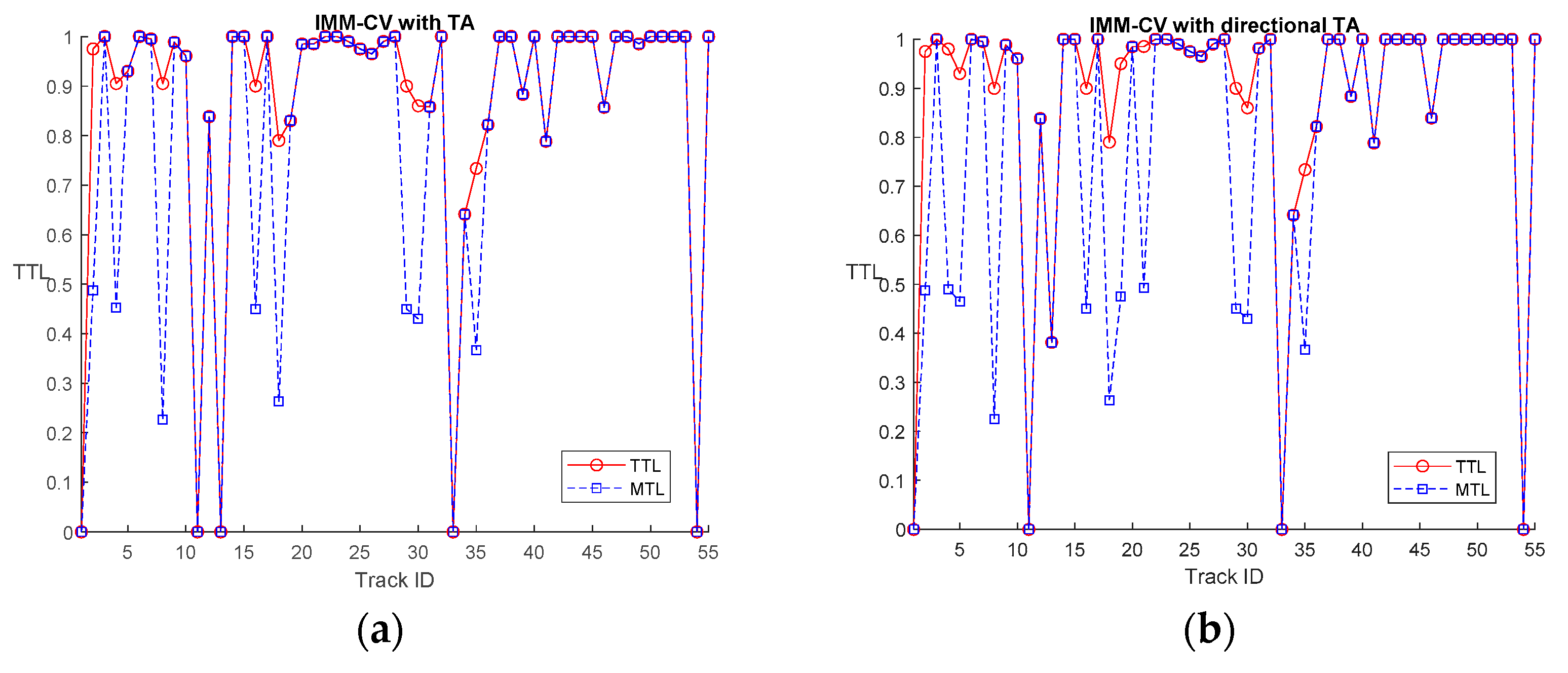
| Avg. TTL | 0.859 | 0.871 | 0.879 | 0.917 |
| Avg. MTL | 0.789 | 0.775 | 0.705 | 0.842 |
| Number of targets with broken tracks | 8 | 9 | 19 | 9 |
| Number of missing targets | 5 | 4 | 3 | 2 |
Publisher’s Note: MDPI stays neutral with regard to jurisdictional claims in published maps and institutional affiliations. |
© 2021 by the author. Licensee MDPI, Basel, Switzerland. This article is an open access article distributed under the terms and conditions of the Creative Commons Attribution (CC BY) license (https://creativecommons.org/licenses/by/4.0/).
Share and Cite
Yeom, S. Long Distance Moving Vehicle Tracking with a Multirotor Based on IMM-Directional Track Association. Appl. Sci. 2021, 11, 11234. https://doi.org/10.3390/app112311234
Yeom S. Long Distance Moving Vehicle Tracking with a Multirotor Based on IMM-Directional Track Association. Applied Sciences. 2021; 11(23):11234. https://doi.org/10.3390/app112311234
Chicago/Turabian StyleYeom, Seokwon. 2021. "Long Distance Moving Vehicle Tracking with a Multirotor Based on IMM-Directional Track Association" Applied Sciences 11, no. 23: 11234. https://doi.org/10.3390/app112311234
APA StyleYeom, S. (2021). Long Distance Moving Vehicle Tracking with a Multirotor Based on IMM-Directional Track Association. Applied Sciences, 11(23), 11234. https://doi.org/10.3390/app112311234