Reinforcement Learning for Options Trading

Abstract

Reinforcement learning has been applied to various types of financial assets trading, such as stocks, futures, and cryptocurrencies. Options, as a novel kind of derivative, have their characteristics. Because there are too many option contracts for one underlying asset and their price behavior is different. Besides, the validity period of an option contract is relatively short. To apply reinforcement learning to options trading, we propose the options trading reinforcement learning (OTRL) framework. We use options’ underlying asset data to train the reinforcement learning model. Candle data in different time intervals are utilized, respectively. The protective closing strategy is added to the model to prevent unbearable losses. Our experiments demonstrate that the most stable algorithm for obtaining high returns is proximal policy optimization (PPO) with the protective closing strategy. The deep Q network (DQN) can exceed the buy and hold strategy in options trading, as can soft actor critic (SAC). The OTRL framework is verified effectively.

1. Introduction

In recent years, reinforcement learning (RL) emerges as an effective way to trade financial assets, such as stocks, futures, and cryptocurrencies. Reinforcement learning, within the financial market, has been gradually dominated by the use of reinforcement learning, in conjunction with other predictive models, such as neural networks [1]. For stock trading, Lei K et al. [2] use historical trading data, features of relevant stocks, and technical analysis indicators as inputs to train a deep reinforcement learning model. The gated recurrent unit (GRU) [3], with a temporal attention mechanism, is utilized to capture long-term dependency. The stacked denoising autoencoders (SDAEs) [4] are employed to denoise the observations, and the asynchronous advantage actor-critic (A3C) model, accompanied with the long short-term memory (LSTM) [5], achieves stable, risk-adjusted returns [6]. Yuming Li et al. [7] put forward a theory of deep reinforcement learning in the stock trading decisions and price predictions. K. Bisht and A. Kumar [8] use multi-objective deep reinforcement learning to get maximum profit by adjusting risk. For future trading, reference [9] uses a time-series momentum and technical indicators to train DQN, policy gradient (PG), and advantage actor-critic (A2C) model. They tested the methods on 50 liquid futures contracts and found that the RL algorithms deliver profits even under high transaction costs. Weiyu Si et al. [10] introduced a multi-objective deep reinforcement learning approach for stock index future’s intraday trading. For cryptocurrency trading, double and dueling DQN is used for trading bitcoin in reference [11], and the trading system produced positive returns. We can see from the above papers that reinforcement learning has been used widely in algorithmic trading.

An option is a contract between two parties in the transaction, regarding the right to buy and sell in the future. The buyer (right party) of an option contract obtains a right by paying a certain fee to the seller (obligation party), that is, the right to buy or sell the agreed amount from the option seller at the agreed time and the agreed price. There are some papers researching options trading or portfolio construction in recent years. Kelly’s criterion is used to construct options portfolio [12]. Zhao L et al. [13] proposed an efficient BSUM-M-based algorithm [14] to solve the portfolio design problem, under the Markowitz mean-variance framework. Reference [15] incorporated volatility forecasting, utilizing investors’ sentiments in the decision-making process, to improve options trading performance. Reference [16] converted index future trading to option trading strategies via LSTM architecture and achieved superior performance.

Although the methods mentioned above demonstrate good performance in options trading or portfolio construction, they are not robust for the actual dynamic market and cannot be directly applied to algorithmic trading. Reinforcement learning agents can interact with the environment and learn the decision-making parameters automatically, which is suitable for trading financial assets, including options trading. However, as far as we know, the papers talking about options trading using reinforcement learning are very few. There are still some problems that need to be solved. First of all, there are many different options contracts for one underlying asset, and each contract has its characteristics. Besides, the period from one contract listed to its expiration is relatively short. Usually, the period is less than six months. The period for active trading is even shorter, usually less than two months. The training of reinforcement learning needs plenty of homogeneous data. Training on one or all contracts cannot meet the demand. Secondly, options, as a kind of derivative, have high leverage and volatility in nature. If the trading of options is not appropriately limited, the principal may suffer a considerable drawdown.

To address the problems mentioned above, we put forward a framework to trade options using reinforcement learning. The underlying asset’s trading data is utilized for training the RL model. Compared with the option contracts, the underlying assets have a more extended and continuous trading period, which is fit for RL training. To further augment the training dataset, we use candle data in different time intervals (a day, 60 min, 30 min, 15 min, and 5 min) to train the model, respectively. Different RL algorithms are used to test our methods, such as DQN, SAC, and proximal policy optimization (PPO). To relieve the volatility of options, we added a protective close strategy to the model. The strategy can prevent unbearable losses. The proposed model was tested on the actual market data for options trading. It can make reliable profits on various options contracts. Furthermore, we compared the models’ performance training on different time interval datasets to find the proper time interval training datasets we should use.

Our study has research significance and application meaning in options algorithmic trading. It has a reference value for other financial assets trading and training data augmentation problems. The main contributions of this paper are as follows:

• We propose a framework to trade options using reinforcement learning. The model is trained on the underlying asset’s trading data. Candle data in different time intervals (a day, 60 min, 30 min, 15 min, and 5 min) are utilized to augment the training datasets. By this means, adequate data is available for training the RL model, leading to a satisfactory result.
• The protective close strategy is added to the RL model to prevent unbearable losses. Due to the high volatility of option prices, the strategy can protect the principal from suffering a massive drawdown. Moreover, the strategy could improve investment returns to some extent.
• The experimental results showed that the proposed model, with the protective close strategy, can get decent returns, compared to the Buy and Hold strategy in options trading, which indicates that our model learns ways to make profit from underlying asset data and applies it to options trading.

The remaining parts of this paper are organized as follows. Section 2 describes the background on reinforcement learning, options trading, and data augmentation. Section 3 introduces the options trading reinforcement learning (OTRL) framework. Section 4 provides experimental settings, results, and evaluation. Finally, Section 5 concludes this paper.

2. Preliminaries and Background

In this section, we first present the introduction to reinforcement learning and algorithmic trading. After that, data augmentation methods for time series are introduced. Finally, we discuss the essential characteristics of the options.

2.1. Reinforcement Learning and Algorithmic Trading

Reinforcement learning is an area of machine learning concerned with how intelligent agents should take actions in an environment to maximize the notion of cumulative reward [17]. Reinforcement learning differs from supervised learning in not needing labeled input/output pairs to be presented and not needing suboptimal actions to be explicitly corrected. Instead, the focus is on finding a balance between exploration and exploitation [18].

Algorithmic trading refers to the method of issuing trading instructions, through the use of computer programs. In trading, the program can determine the choice of trading time, price of the transaction, and even number of securities that need to be traded in the end. Algorithmic trading, also called quantitative trading, is a subfield of finance, which can be viewed as the approach of automatically making trading decisions based on a set of mathematical rules computed by a machine [19].

Applying reinforcement learning to algorithmic trading is a significant improvement. The RL model can learn its trading strategy by observing the market environment and trying different actions, not like supervised learning that trains a predictive model on historical data to forecast the trend direction. If we get a predictive model trained by LSTM, we still need to develop a trading strategy to utilize its forecasting result, and the risk of error needs to be considered. However, for reinforcement learning, we need to input adequate and appropriate data. The specified model can learn the trading strategy that concerns the long-term rewards, not just short-term rewards. Besides this, the RL model can update its strategy automatically, according to new observations.

2.2. Data Augmentation Methods for Time Series

Data augmentation has proven to be an effective approach to reduce over-fitting and improve generalization in the neural network [20]. By assuming that more information can be extracted from the dataset through augmentations, it further has the advantage that it is a model-independent solution [21]. In tasks such as image recognition, data augmentation is a common practice and may be seen as a way of pre-processing the training set only [22]. However, such augmentation strategies are not easily extended to time-series data, in general, due to the non-independent and identically distributed (i.i.d.) property of the measurements forming each time series [23]. For the financial time series, Teng et al. [24] used a time-sensitive data augmentation method for stock trend prediction, where data is augmented by corrupting high-frequency patterns of original stock price data, as well as preserving low-frequency ones in the frame of discrete wavelet transform (DWT) [25].

Data augmentation for time series is still an open research field. There are some methods put forward to tackle the problem, such as magnify [26], jittering [27], and SPAWNER [28]. Fons et al. [23] evaluated the performance of these methods for financial time series classification.

2.3. Basic Characteristics of Options

Options are a type of financial derivative. Its underlying instrument can be a stock, index, currency, commodity, exchange traded fund (ETF), or any other security. An option contract gives an investor the right to either buy or sell an asset at a pre-determined price by a specific date. There are two types of options, call options and put options. A call option gives its owner the right to buy the underlying asset, while a put option gives its owner the right to sell the underlying asset.

The strike price is the price for which the option’s owner can buy or sell the underlying asset. There are usually at least several different strike prices available for one underlying and one type of option (calls or puts). For example, for Shanghai 50 ETF (510050), which currently trades at 3.5, you can trade call options with strike prices of 3.4, 3.5, 3.6, 3.7, etc., and put options with the strike prices of 3.3, 3.4, 3.5, 3.6, etc.

3. Methodology

In this section, we introduce the options trading reinforcement learning (OTRL) framework and its protective close strategy. Section 3.1 presents the training data for the RL model trading options. Section 3.2 details the OTRL framework, and Section 3.3 introduces the algorithms used in the framework. Section 3.4 introduces the protective close strategy that the framework utilizes.

3.1. Training Data for Options Trading

Options trading data are challenging to use in RL training directly, due to two aspects. The first one is that there are many different options contracts for one underlying asset, and each contract has its characteristics of price behavior. It is hard to construct a unified dataset from different options contracts for RL training. The second problem is that the period from one contract listed to its expiration is relatively short. RL training requires a great deal of data with similar characteristics. If the trading data of one contract is used to train the RL model, its amount is not enough. Selecting a proper dataset to train the RL model is a crucial problem for algorithmic options trading.

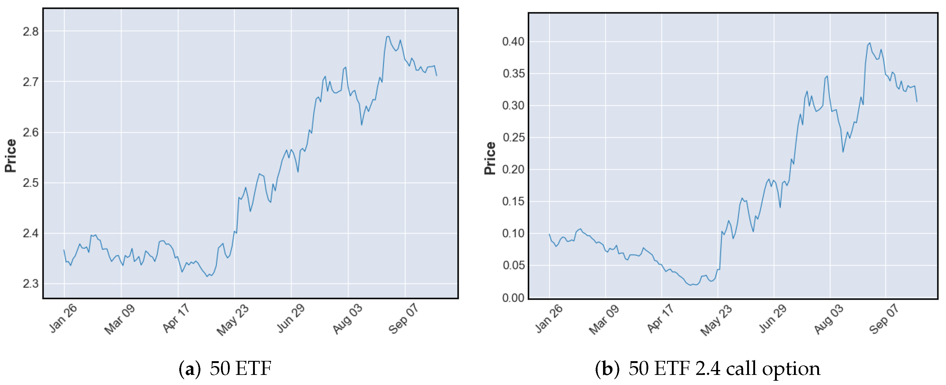
To solve the problem mentioned above, we find that the underlying asset’s trading data can train the RL model. In our experiment, we use trading data of Shanghai 50 ETF and Shanghai and Shenzhen 300 ETF (510300) to train the RL model. They are the only two ETFs that have exchange-traded option contracts in the A-share market. Figure 1 shows a close price trend of 50 ETF, from 26 January 2017 to 27 September 2017, and its 2.4 call option. 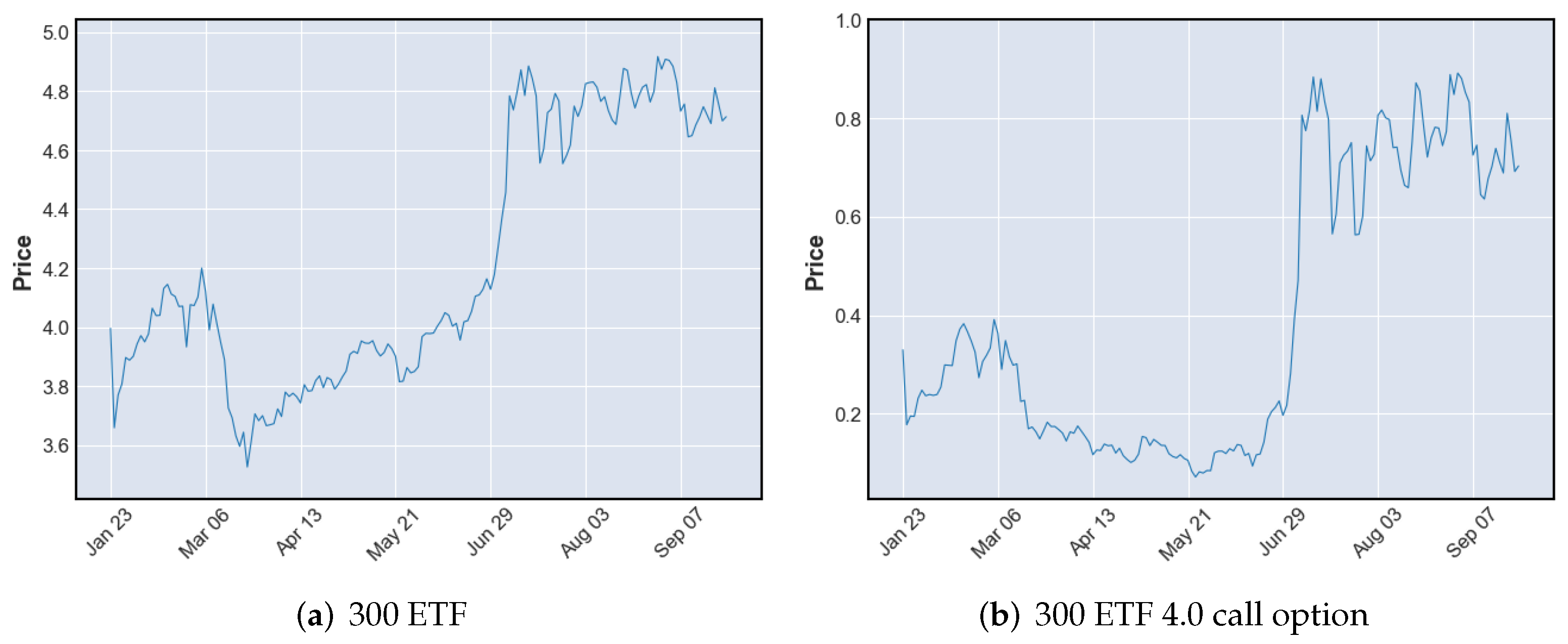Figure 2 shows a close price trend of 300 ETF, from 23 January 2020 to 23 September 2020, and its 4.0 call option. The period is from the option listed date to its expiration date. As shown in the two figures, the price behavior of the option and its underlying asset are very similar. As a result, the experience learned from the underlying asset trading data can be used in trading its option contracts. Furthermore, the underlying asset trading data is more extended and continuous, which is more suitable for RL training.

However, the daily trading of the data of underlying assets is not very sufficient for RL training in reality. Shanghai 50 ETF was listed on the exchange on 23 February 2005. Additionally, Shanghai and Shenzhen 300 ETF was listed on the exchange on 28 May 2012. There are about 250 trading days in a year. Thousands of daily trading data rows are not enough to train the RL model, which needs millions of steps to converge. It may lead to over-fitting. To further augment the training dataset, we use the underlying asset candle data in different time intervals (a day, 60 min, 30 min, 15 min, and 5 min) to train the RL model, respectively. Minute candle data can be used to train RL agents for data augmentation [29]. The agent is then used to guide daily trading. The data in a larger time interval (like 60 min) may be more similar to daily data in price behavior, but its amount is fewer and vice versa. In our experiment, proper training data can be picked out from data in different time intervals.

The trading data we used to train the RL model contains five columns: open price, highest price, lowest price, close price, and trading volume. Trading data in different time intervals all have these features. When multiple features exist simultaneously, if the range of feature values is very different, the feature with a more extensive value range is more likely to significantly impact the model, such as the trading volume in our training data. Normalization is to process the data by some algorithm and then limit it to a specific range. In our experiment, the features mentioned above were normalized to a dataset with a mean of 0 and variance of 1. The normalization formula is as follows:

$$z=\frac{x-\mu }{\sigma }$$

(1)

Among which, $\mu$ and $\sigma$ are the mean and variance of the original dataset, respectively. Due to the large fluctuations in the stock price and the options price, it is more reasonable to normalize the features by a certain length of a sliding window, rather than normalize the global features data.

3.2. Proposed OTRL Framework

The proposed OTRL framework uses underlying asset trading data in different time intervals to train the RL model. A standard reinforcement learning environment usually contains state, action, reward, and done or not. For financial assets, our state includes time, open price, highest price, lowest price, close price, and trading volume [30]. At every step, the agent can take one of the following actions:

• Do nothing: skip the bar without taking an action.
• Buy an asset: if the agent has already got the asset, nothing will be bought; otherwise, we will pay the commission (0.1% by default).
• Close the position: if we do not have a previously purchased asset, nothing will happen; otherwise, we will pay the commission of the trade.

The training will use several RL algorithms, i.e., DQN, PPO, and SAC, in our experiment. PPO and SAC will be introduced in Section 3.3. After the training, different models training on datasets in different time intervals are applied to trade underlying assets for validation. The model behaving well will be selected by trading on datasets that are different from the training datasets. By this means, the training dataset in the proper time interval is confirmed in different RL algorithms. Then, the selected model is used for trading options contracts.

There are many options contracts for one underlying asset. For example, Shanghai 50 ETF option quotation on one day is listed in

Table 1. 50 ETF option quotation.

Call	Strike Price	Put
0.2091	3.2	0.0055
0.1184	3.3	0.0184
0.0530	3.4	0.0509
0.0193	3.5	0.1170
0.0063	3.5	0.2079

.

Table 2. 50 ETF call option candle data.

Strike Price	Open	Highest	Lowest	Close
3.3	0.1671	0.1709	0.1126	0.1184
3.4	0.0876	0.0900	0.0496	0.0530
3.5	0.0379	0.0390	0.0180	0.0193

shows the 50 ETF call option candle data that day. The close price of 50 ETF that day was 3.399. In our experiment, the model trades one option contract in one test, to show a complete trading result on one contract during a specific period. In reality, the agent can monitor many options contracts at the same time. We can buy the option contract that the agent takes a buy action on early, in order to seize the trading opportunity in time.

3.3. Primary Algorithm Introduction

DQN, PPO, and SAC are typical reinforcement learning algorithms. They are used to verify the effectiveness of the data augmentation method. Details of the three algorithms are as follows.

3.3.1. Q-Learning and DQN

Methods in this Q-learning family learn an approximator $Q(s,a)$ for the optimal action-value function, $Q^{*}(s,a)$. Typically they use an objective function, based on the Bellman equation. This optimization is almost always performed off-policy, which means that each update can use data collected at any point during training, regardless of how the agent was chosen to explore the environment when the data was obtained. The corresponding policy is obtained via the connection between $Q^{*}$ and ${\pi }^{*}$: the actions taken by the Q-learning agent are given by:

$$a\left(s\right)=arg\underset{a}{max}Q(s,a).$$

(2)

DeepMind successfully trains DQN on a set of 49 Atari games and demonstrates the efficiency of the approach, when applied to complicated environments [31]. The steps of the DQN algorithm are shown in Algorithm 1.

Algorithm 1: DQN.

Initialize the parameters for $Q(s,a)$ and $\stackrel{target}{Q}(s,a)$ with random weights and empty the replay buffer. With probability $ϵ$, select a random action a, otherwise, $a\left(s\right)=arg\underset{a}{max}Q(s,a)$. Excute action a in an emulator and observe the reward r and the next state $s^{{}^{\prime }}$. Store transition $(s,a,r,s^{{}^{\prime }})$ in the replay buffer. Sample a random mini-batch of transitions from the replay buffer. For every transition in the buffer, calculate target $y=r$ if the episode has ended at this step, or $y=r+\gamma \underset{a^{{}^{\prime }}\in A}{max}\stackrel{target}{Q}(s,a)$. Calculate loss: $L={(Q(s,a)-y)}^2$. Update $Q(s,a)$ using the stochastic gradient descent algorithm by minimizing the loss in respect to the model parameters. Every N steps, copy weights from Q to $\stackrel{target}{Q}$. Repeat from step 2 until converged.

3.3.2. Proximal Policy Optimization

PPO is motivated by the same question of trust region policy optimization (TRPO) [32]. How can we take the biggest possible improvement step on a policy using the data we currently have, without stepping so far that we accidentally cause performance collapse? TRPO tries to solve this problem with a complicated second-order method. PPO is a family of first-order methods that use a few other tricks to keep new policies close to old.

PPO updates policies via:

$${\theta }_{k+1}=arg\underset{\theta }{max}\underset{s,a\sim {\pi }_{{\theta }_k}}{\mathrm{E}}\left[L(s,a,{\theta }_k,\theta )\right],$$

(3)

typically taking multiple steps of (usually minibatch) SGD to maximize the objective. Here, L is given by:

$$L(s,a,{\theta }_k,\theta )=min\left(\frac{{\pi }_{\theta }\left(a\right|s)}{{\pi }_{{\theta }_k}\left(a\right|s)}{A}^{{\pi }_{{\theta }_k}}(s,a),\mathrm{clip}\left(\frac{{\pi }_{\theta }\left(a\right|s)}{{\pi }_{{\theta }_k}\left(a\right|s)},1-ϵ,1+ϵ\right)A^{{\pi }_{{\theta }_k}}(s,a)\right),$$

(4)

in which $ϵ$ is a (small) hyperparameter, which roughly says how far away the new policy is allowed to go from the old.

There is another simplified version of this objective:

$$L(s,a,{\theta }_k,\theta )=min\left(\frac{{\pi }_{\theta }\left(a\right|s)}{{\pi }_{{\theta }_k}\left(a\right|s)}{A}^{{\pi }_{{\theta }_k}}(s,a),g(ϵ,A^{{\pi }_{{\theta }_k}}(s,a))\right),$$

(5)

where

$$g(ϵ,A)=\left\{\begin{array}{cc}(1+ϵ)A\hfill & A\ge 0\hfill \\ (1-ϵ)A\hfill & A<0.\hfill \end{array}\right.$$

(6)

Clipping serves as a regularizer, by removing incentives for the policy to change dramatically. The hyperparameter $ϵ$ corresponds to how far away the new policy can go from the old, while still profiting the objective.

3.3.3. Soft Actor-Critic

SAC is an algorithm that optimizes a stochastic policy in an off-policy way. A central feature of SAC is entropy regularization. The policy is trained to maximize a trade-off between expected return and entropy, a randomness measure in the policy. Increasing entropy results in more exploration, which can accelerate learning later on. It can also prevent the policy from prematurely converging to a bad local optimum.

Entropy is a quantity that says how random a random variable is. Let x be a random variable, with probability mass P. The entropy H of x is computed from its distribution P, according to:

$$H\left(P\right)=\underset{x\sim P}{\mathbb{E}}\left[-logP\left(x\right)\right].$$

(7)

In entropy-regularized reinforcement learning, the agent gets bonus rewards at each timestep. This changes the RL problem to:

$${\pi }^{*}=arg\underset{\pi }{max}\underset{\tau \sim \pi }{\mathbb{E}}\sum _{t=0}^{\infty }{\gamma }^t\left(R(s_t,a_t,s_{t+1})+\alpha H\left(\pi (·|s_t)\right)\right),$$

(8)

where $\alpha >0$ is the trade-off coefficient. The policy of SAC should, in each state, act to maximize the expected future return, plus expected future entropy.

Original SAC is for continuous action settings and it is not applicable to discrete action settings. To deal with discrete action settings of our financial asset, we use an alternative version of the SAC algorithm that is suitable for discrete actions. It is competitive with other model-free, state-of-the-art RL algorithms [33].

3.4. Protective Closing Strategy

The protective closing strategies are independent mechanisms, intended to prevent unbearable losses [34]. Under the stop-loss mechanism, all positions are immediately closed if the unrealized loss exceeds the threshold. For example, if the threshold is set to 2% and we take a long position at 5.0, once the price dropped to below 4.9, then the stop-loss mechanism would be triggered, such that the position would be closed immediately.

There is a take-profit mechanism being used to ensure that a profit is realized in reference [34]. Once the gain reaches the threshold, the take-profit mechanism is activated to protect unrealized gain. In our experiment, trading actions depended on the RL agent. We used the stop-loss mechanism to prevent unbearable losses in options trading. Ideally, the take-profit mechanism can be learned by the agent from the training process. Therefore, we do not use the take-profit mechanism in the OTRL framework explicitly.

For the stop-loss mechanism, we need to determine the threshold value that means the maximum loss a trader can accept in one complete trade. In our experiment, we use the validation dataset to select the proper stop-loss threshold. The validation dataset contains the underlying asset and option daily trading data. The trading period of the underlying asset in the validation dataset is different from the training dataset.

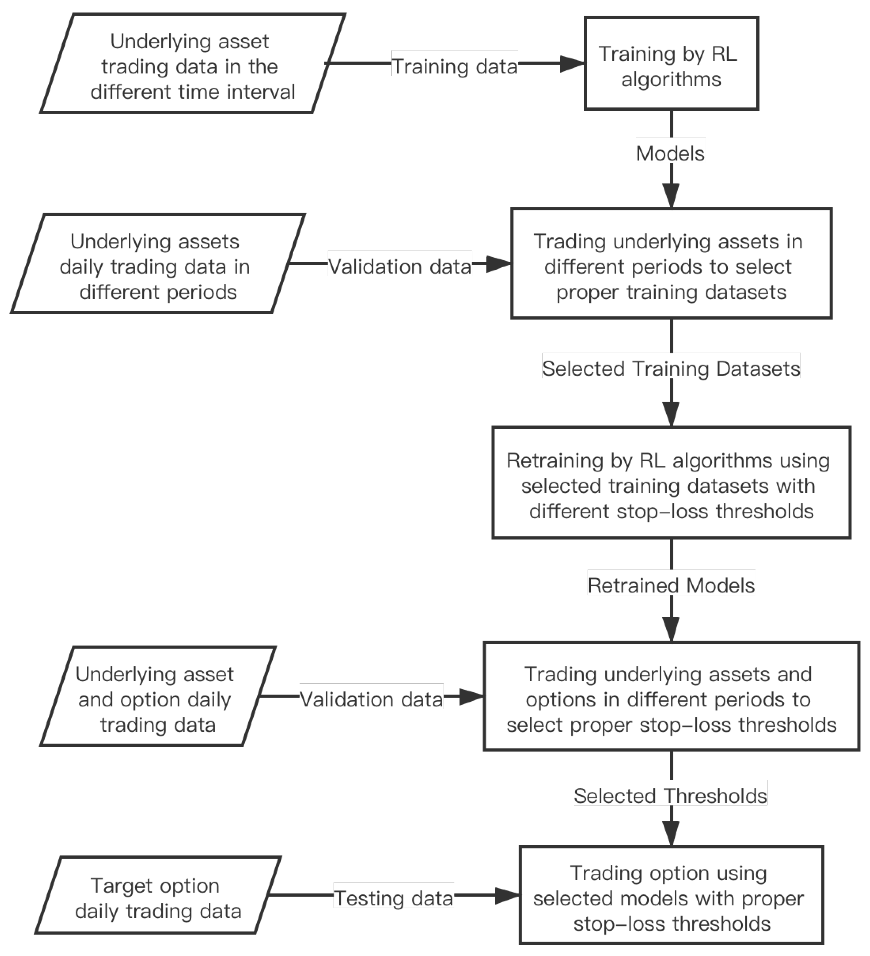
The proposed OTRL framework is illustrated in Figure 3. Firstly, the underlying asset trading data in different time intervals (a day, 60 min, 30 min, 15 min, and 5 min) are used to train RL models. Different RL algorithms can be applied, such as DQN, PPO, and SAC, in our experiment. After the training, the models are used for trading underlying assets in different periods to select training data in a proper time interval, such as 60-min trading data. Then, the selected training data are used to retrain the model with different stop-loss thresholds. Afterward, the retained models are used for trading underlying assets and options in different periods, in order to select the proper stop-loss thresholds. Finally, the retrained models, with proper stop-loss thresholds, are used for trading options in the testing dataset.

4. Experiment Result

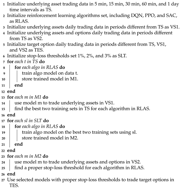
To evaluate the effectiveness of the proposed OTRL framework, we designed an experiment process, referring to Algorithm 2. Firstly, the better time interval of trading data is selected by the training and validation process. Secondly, the proper threshold of the protective closing strategy is determined by the retraining and validation process. Thirdly, the final models are used for trading options.

4.1. Training Result

In our experiment, we used 50 ETF trading data from 5 January 2009 to 25 January 2017 and 300 ETF trading data from 28 May 2012 to 22 January 2020, in different time intervals (a day, 60 min, 30 min, 15 min, and 5mins), as training sets. Transaction costs were set as 0.1% (buy and sell were the same). The reinforcement learning framework we used was SLM-Lab (https://github.com/kengz/SLM-Lab, accessed on 10 November 2021). We used DQN, PPO, and SAC to train the trading agents in our experiments.

The agents were initialized with five normalized inputs (open price, highest price, lowest price, close price, and trading volume), two hidden fully-connected layers (512-512), and three outputs (buy, hold, and sell). By using the SLM-Lab, one experiment was a trial in the framework. Additionally, a trial contained four concurrent sessions. Each session included the same algorithm structure and different initialized random parameters. The parameters of the DQN, PPO, and SAC models are shown in

Table 3. Hyperparameters setting.

Parameter	Parameter Description	Value
net_type	Type of the neuron network	fully-connected network
batch_size	Batch size	32
loss_func	Loss function	MSE loss
optimizer	Optimization method	Adam
lr	Learning rate	0.00025
DQN max_frame	Training steps of DQN	6,000,000
PPO max_frame	Training steps of PPO	10,000,000
SAC max_frame	Training steps of SAC	5,000,000
replay_buffer	Max size of replay buffer	1,000,000

.

Algorithm 2: OTRL Framework.

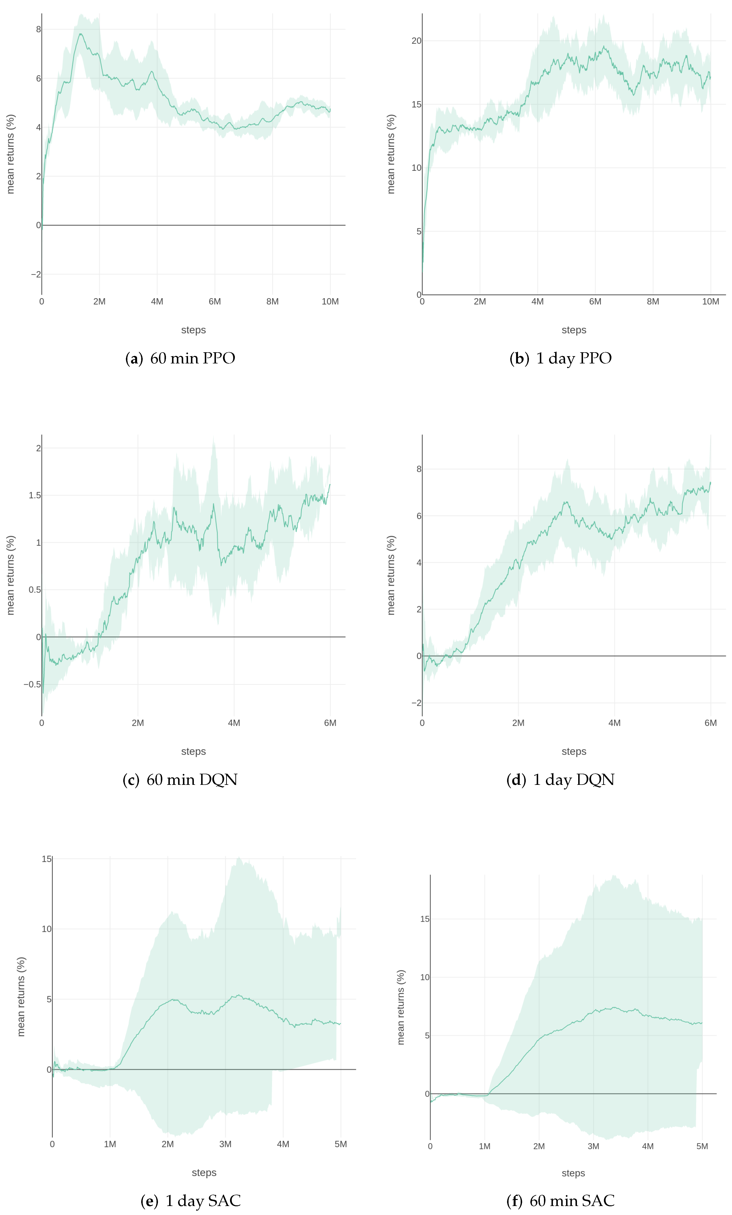
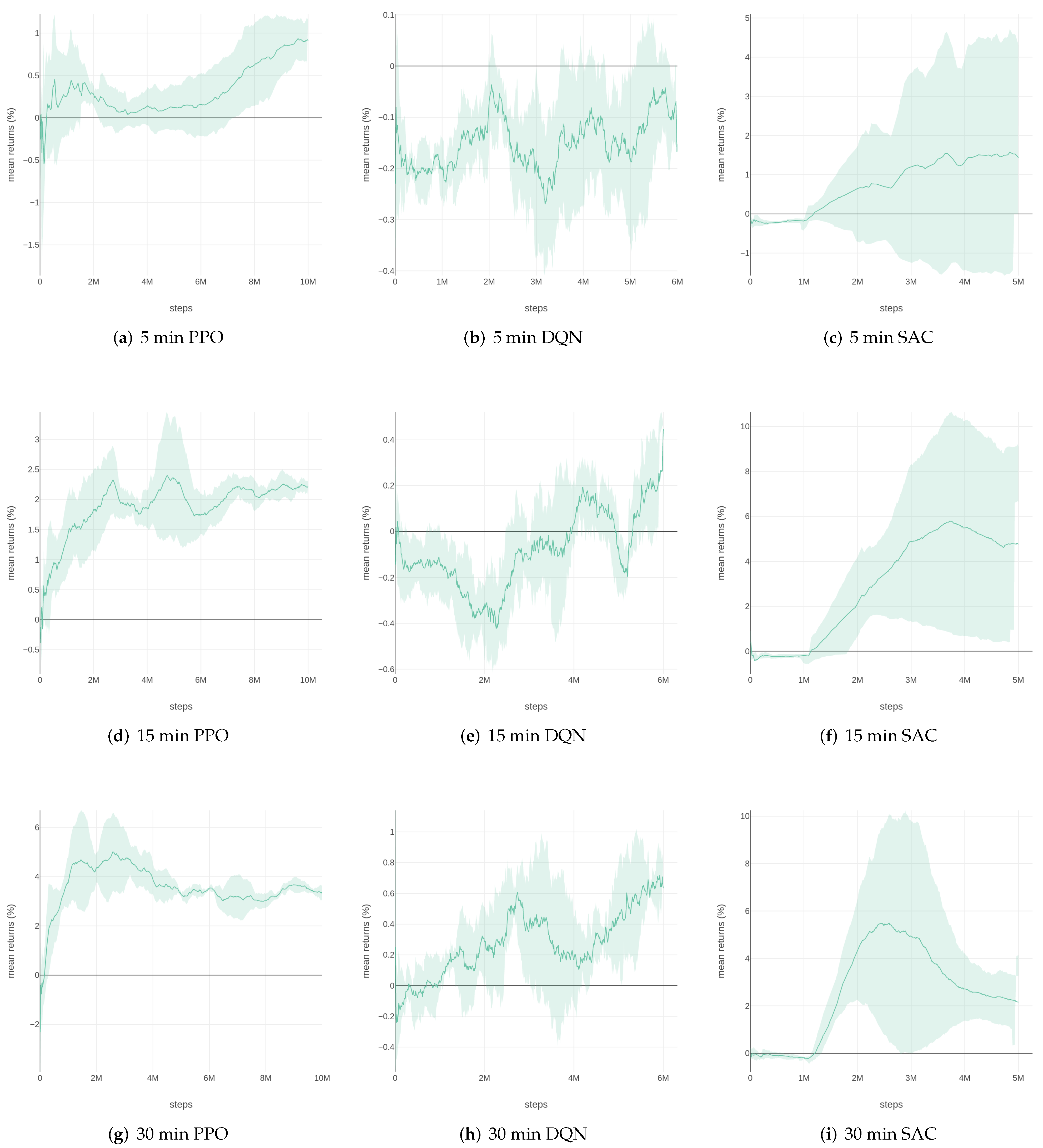
Figure 4 and Figure 5 show the training results of 50 ETF, in five different time intervals, using the three RL algorithms. A trial graph takes the mean of sessions and plots an error envelop using standard deviation. As we can see from Figure 4, the models trained on the dataset in larger time intervals (such as 60 min or 1 day) tend to perform better in training results. There is more noise than in the trading data of shorter time intervals (like 5 min or 15 min). It is difficult for models to learn a pattern using training data with too much noise. However, limited training data may lead to overfitting. To select a proper time interval for training data, we use models trained on 60-min and 1-day trading data for the validation process.

4.2. Validation Result

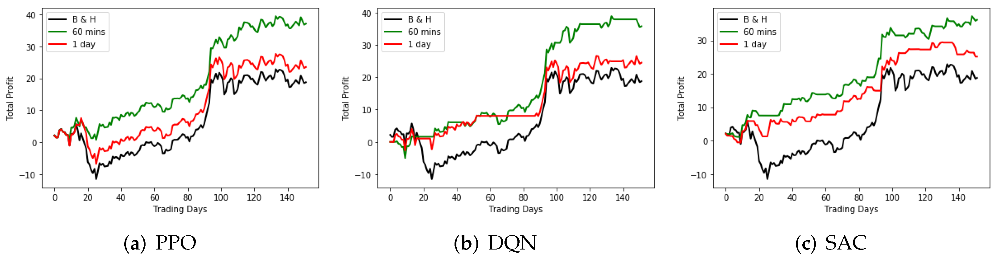
To verify the effectiveness of the models, we use them for trading the assets on different trading dates from the training dataset. Validation sets contain 50 ETF trading data from 22 February 2017 to 30 March 2021, as well as 300 ETF trading data from 23 January 2020 to 23 September 2020. Figure 6 and Figure 7 show the trading performance of the agents trained on 60-min and 1-day trading data, using the three algorithms, compared with the buy and hold (B and H) strategy.

From Figure 6 and Figure 7, we can see that the agents trained on 60-min trading data surpass the agents trained on 1-day trading data and B and H strategy among the three algorithms. The agents trained on 1-day trading data do not always outperform the B and H strategy on the validation sets, and they perform well on the training sets. The amount of 1-day trading data training sets is a quarter of that of the 60-min trading data training set. We infer that the poor performance of the agents trained on 1-day trading data was due to overfitting. In addition, the agents trained using PPO tend to hold the asset and reduce trading frequency. While the agents trained using DQN tend to have no position and wait for trading opportunities. Furthermore, the agents trained using SAC tend to trade frequently or even randomly.

The validation results show that the agents, trained on 60-min trading data, using the three algorithms, perform well on trading assets in different trading dates from the training dataset, which verifies their effectiveness. To further improve the performance of trading options, the protective closing strategy is added to the models in the next stage.

4.3. Trading Performance with Protective Closing Strategies

To better apply the models to option trading, we need to add a protective closing strategy to the training stage. In our experiment, the alternative stop-loss thresholds were 1%, 2%, and 3%. If the loss of one step exceeded the threshold, all positions were immediately closed. The mechanism can prevent unbearable losses, especially in options trading.

In the preceding validation process, we found that the models trained on 60-min trading data performed better on the validation set and surpassed the B and H strategy. Therefore, the training for threshold selection used 60-min trading data as the training set. From the

Table 4. Trading performance with different stop-loss thresholds.

Assets	Model	Thresholds	Mean Returns
50 ETF	DQN	1%	1.32%
50 ETF	DQN	2%	1.98%
50 ETF	DQN	3%	1.56%
50 ETF	PPO	1%	3.87%
50 ETF	PPO	2%	4.74%
50 ETF	PPO	3%	4.06%
300 ETF	DQN	1%	0.95%
300 ETF	DQN	2%	1.37%
300 ETF	DQN	3%	1.04%
300 ETF	PPO	1%	3.67%
300 ETF	PPO	2%	4.31%
300 ETF	PPO	3%	3.91%

, we can see that 2% is the better threshold for the PPO and DQN models. The protective closing strategy was unsuitable for the SAC models. That may be because the SAC models have their own stop-loss mechanism in the frequent and even random trading mode. Because the SAC models trade frequently, they can not benefit from long-term holding. Under this condition, the protective closing strategy shortens the holding time further, which tends to reduce the returns, rather than lowering the risk.

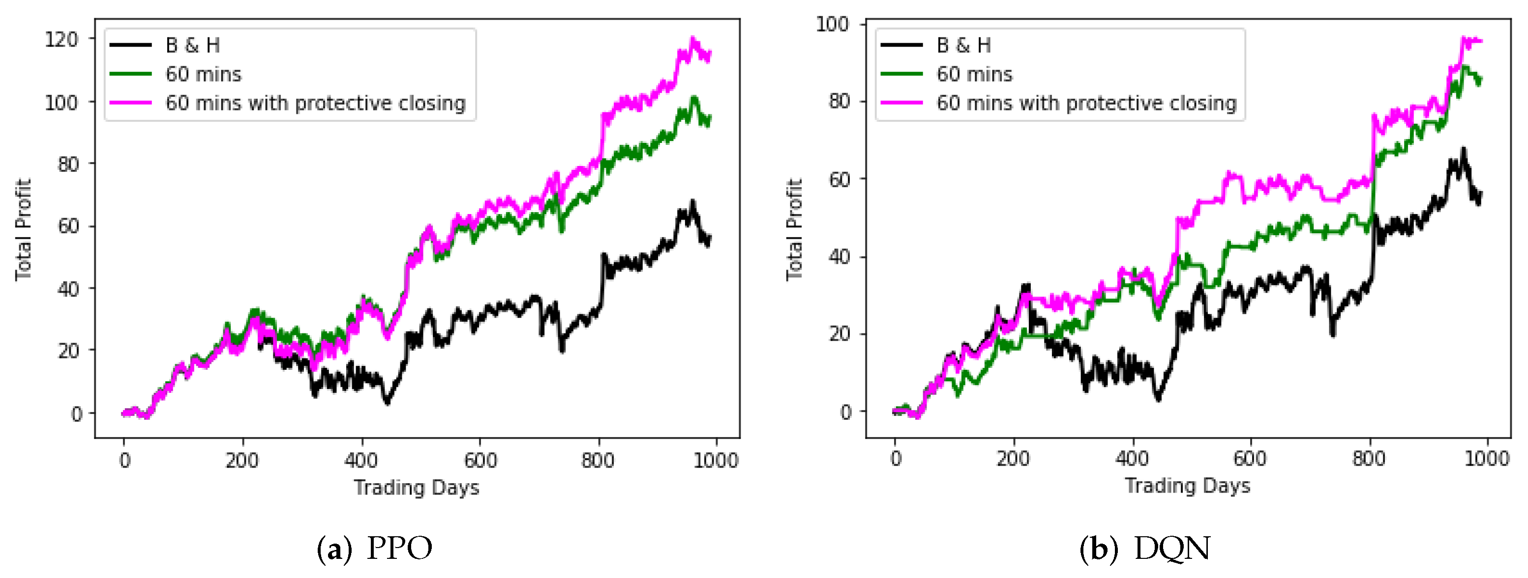
Figure 8 and Figure 9 show the trading performance of the agents with and without the protective closing strategy, compared with the B and H trading strategy. The validation set is the same as the one in the previous section. From Figure 8 and Figure 9, we can see that the protective closing strategy does not lower the returns while reducing the risk of unbearable losses, which is especially important for options trading.

Since the models with the protective closing strategy performed well on the validation set, they can be applied to trade options in the next stage. Although the SAC model cannot be trained well with protective closing strategy, it is still used to trade options, for comparison.

4.4. Trading Performance on Options

Having determined the training data and chosen the proper stop-loss threshold, we can eventually apply the model to trading options. In our experiment, the underlying assets of the options were 50 and 300 ETF. The options were traded using the models trained on respective underlying assets trading data. The trading dates of the testing set were different from those of the training set.

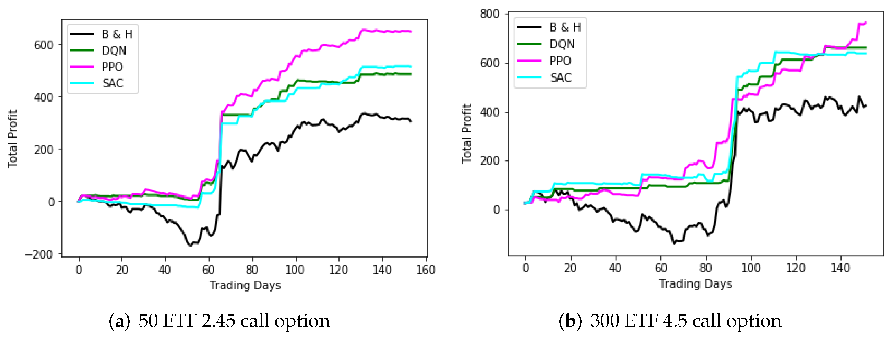
Figure 10 shows trading performance on options of 50 and 300 ETF. The option in Figure 10a was 2.45 call of 50 ETF from 26 January 2017 to 27 September 2017. The option in Figure 10b was 4.5 call of 300 ETF from 23 January 2020 to 23 September 2020. The DQN and PPO models were trained with a 2% stop-loss threshold, and they were used for trading options with the same threshold. The SAC model was trained without a protective closing strategy, but it was used to trade options with a 2% stop-loss threshold, for comparison. From Figure 10 and

Table 5. Trading performance on different options.

Options	Model	Annualized Return	Sharpe Ratio
50 ETF 2.45 call	B and H	608.94%	32.56
50 ETF 2.45 call	DQN	969.05%	58.61
50 ETF 2.45 call	PPO	1294.68%	76.34
50 ETF 2.45 call	SAC	1027.28%	62.40
300 ETF 4.5 call	B and H	848.68%	34.79
300 ETF 4.5 call	DQN	1322.01%	72.03
300 ETF 4.5 call	PPO	1524.88%	100.36
300 ETF 4.5 call	SAC	1274.94%	67.70

, we can see that the RL models with protective closing strategy outperformed the B and H trading strategy, which verifies the effectiveness of our OTRL framework. In addition, the PPO model performed best among the three models, which is likely due to the fact that its internal strategy of holding goes well with the stop-loss mechanism in trading options.

5. Conclusions

In this paper, we propose the OTRL framework to trade options using RL algorithms. It provides a set of executable processes, including training, validation, and testing processes. Underlying assets’ trading data in different time intervals were used as the training set. In our experiment, PPO, DQN, and SAC were chosen to train the models. In practice, any RL algorithms can be applied to trading options using the OTRL framework. Trading data options of 50 and 300 ETF, in the A-share market, was used as the testing set. The models with a protective closing strategy performed well on options trading, compared with the B and H trading strategy, which verifies the effectiveness of the OTRL framework. It addresses the problem of lack of training data and reduces trading risk. The PPO model with a protective closing strategy performed best among the three models, which may have a reference value for the following research.

While the proposed framework has been verified effectively, some directions are still worth studying in the future. Multi-leg options strategies can be considered to reduce trading risk further. Meta learning may be utilized to train the model using options with different strike prices simultaneously.