Article

Simulated Annealing-Based Hyperspectral Data Optimization for Fish Species Classification: Can the Number of Measured Wavelengths Be Reduced?

1
School of Electrical Engineering and Computer Science, University of North Dakota, Grand Forks, ND 58202, USA
2
SafetySpect Inc., Los Angeles, CA 90067, USA
3
USDA/ARS Environmental Microbial and Food Safety Laboratory, Beltsville Agricultural Research Center, Beltsville, MD 20705, USA
4
Food Science Program, Schmid College of Science and Technology, Chapman University, 1 University Drive, Orange, CA 92866, USA
*
Author to whom correspondence should be addressed.
Appl. Sci. 2021, 11(22), 10628; https://doi.org/10.3390/app112210628
Submission received: 12 September 2021 / Revised: 31 October 2021 / Accepted: 8 November 2021 / Published: 11 November 2021

Abstract

:
Relative to standard red/green/blue (RGB) imaging systems, hyperspectral imaging systems offer superior capabilities but tend to be expensive and complex, requiring either a mechanically complex push-broom line scanning method, a tunable filter, or a large set of light emitting diodes (LEDs) to collect images in multiple wavelengths. This paper proposes a new methodology to support the design of a hypothesized system that uses three imaging modes—fluorescence, visible/near-infrared (VNIR) reflectance, and shortwave infrared (SWIR) reflectance—to capture narrow-band spectral data at only three to seven narrow wavelengths. Simulated annealing is applied to identify the optimal wavelengths for sparse spectral measurement with a cost function based on the accuracy provided by a weighted k-nearest neighbors (WKNN) classifier, a common and relatively robust machine learning classifier. Two separate classification approaches are presented, the first using a multi-layer perceptron (MLP) artificial neural network trained on sparse data from the three individual spectra and the second using a fusion of the data from all three spectra. The results are compared with those from four alternative classifiers based on common machine learning algorithms. To validate the proposed methodology, reflectance and fluorescence spectra in these three spectroscopic modes were collected from fish fillets and used to classify the fillets by species. Accuracies determined from the two classification approaches are compared with benchmark values derived by training the classifiers with the full resolution spectral data. The results of the single-layer classification study show accuracies ranging from ~68% for SWIR reflectance to ~90% for fluorescence with just seven wavelengths. The results of the fusion classification study show accuracies of about 95% with seven wavelengths and more than 90% even with just three wavelengths. Reducing the number of required wavelengths facilitates the creation of rapid and cost-effective spectral imaging systems that can be used for widespread analysis in food monitoring/food fraud, agricultural, and biomedical applications.

1. Introduction

Over the past 20 years, hyperspectral imaging (HSI) has become an invaluable tool for food safety and quality applications [1,2]. Spoilage and contamination of food and agricultural products are ongoing concerns for the food industry. Recent applications of hyperspectral imaging for food safety include detection of mold in peanuts [3,4], lead pollution in lettuce leaves [5], and Fusarium head blight in wheat kernels and wheat flour [6]. Food fraud, the intentional misrepresentation of food or food ingredients for economic gain, is another major food safety issue that has been addressed with hyperspectral imaging. For example, this technology has been applied for identifying fillets of less expensive species of fish that have been marketed and sold as more expensive red snapper (Lutjanus campechanus) fillets [7,8].
Hyperspectral imaging has been a staple of agriculture monitoring, with initial applications dating back to the 1970s. Early applications include large-scale remote monitoring of land and agriculture from the Landsat-I satellite [9], monitoring of crop yield [10], and detection of plant disease and invasive species [11]. While agriculture applications have remained constant since these early examples, the methods have changed with new technologies enabling more localized analysis. Unmanned aerial vehicles (UAVs) have become attractive survey platforms for local, detailed aerial monitoring efforts [12] and advancements in computing technology and miniaturization of HSI devices have enabled the construction of new systems for in-field crop analysis [13].
Hyperspectral imaging devices are complex systems that can be characterized by the method with which the full spatial-spectral data cube is obtained. Data cubes can be acquired by spatial scanning, spectral scanning, or by a combination of these methods [14]. With spatial scanning imagers, light is collected at a point or along a line and dispersed into its spectral components by a dispersive optic such as prism or diffraction grating. This point or line is then scanned over the target area through the physical motion of the sensor, reflection from a scanning mirror, or physical motion of the target object. With spectral scanning imagers, the full spatial content is collected by the image sensor for individual wavelengths in sequence. Collection of the wavelengths is typically accomplished by switching wavelengths through filter wheels, electronically controlled liquid crystal tunable filters (LCTF), or acousto-optic tunable filters (AOTF) [15].
Despite successes in the food safety and agriculture industries, hyperspectral imaging does have disadvantages, mostly due to the data cube being constructed from individual components collected in a time-sequential manner. This can be an error-prone process, especially for high-speed imaging applications. Another category of the hyperspectral imager, the snapshot imager, overcomes these issues by combining an array of optics to collect both the spatial and spectral information simultaneously. Usually, this means some compromise in either the spectral or spatial domain. All of these solutions tend to be both complex and costly [16]. In research and discovery, it is unknown which wavelengths will be significant and which are redundant. In many cases, once the spectral characteristics for a particular targeted application are understood, there can be a significant reduction in the complexity of the spectral imaging system.
Issues common to all hyperspectral imager types are the significant computing power required and the large file sizes of the data cubes, especially in applications involving larger fields of view. Attempts to address these issues have included the application of compressive sensing [17,18,19], deep neural networks [20], and methods centered around principal component analysis (PCA) [21]. Each of these solutions has its own limitations in terms of heavy computational requirements and large file sizes for data cube analysis.
This paper shows proof of concept for a new method for selecting narrow wavelengths for the classification of material samples. This method could support the design of a hypothetical rapid spectral imaging system consisting of a focal plane array covered with a mosaic color filter array or illumination by selected wavelength LEDs. These can collect full spatial resolution images at a small number of narrow wavelengths for visible/near-infrared (VNIR), shortwave infrared (SWIR) reflectance, and fluorescence. The proposed method has the potential to be applied in a hand-held, mobile device for rapid scanning of food products in wholesale or retail marketplaces or configured as a drone-deployable payload for low-altitude aerial scanning of crops and vegetation.
The aim of this study was to evaluate the potential of this new method for use in an application combating food fraud by determining the correct species of fish fillets that are often mislabeled to justify a higher selling price [8,22]. Specific objectives were to (1) develop and evaluate a heuristic wavelength selection algorithm, (2) develop and evaluate methods for classifying the species of a fillet using classifiers designed for both single-mode spectroscopy and a fusion of spectroscopy modes, and (3) compare the relative effectiveness of each spectral mode for this classification task.

2. Materials and Methods

2.1. Hyperspectral Imaging Systems

Full-resolution reflectance and fluorescence images were collected using an in-house developed visible and near-infrared (VNIR) hyperspectral imaging system [23]. The light source for the VNIR reflectance was a 150 W quartz tungsten lamp (Dolan Jenner, Boxborough, MA, USA). For fluorescence imaging, two UV narrowband light sources were used, each with four 10 W, 365 nm, LEDs (LED Engin, San Jose, CA, USA). VNIR reflectance images in 125 wavelengths within the 419–1007 nm spectral range and fluorescence images in 60 wavelengths within the 438–718 nm range were acquired using a 23 mm focal length lens, an imaging spectrograph (Hyperspec-VNIR, Headwall Photonics, Fitchburg, MA, USA), and a 14-bit electron-multiplying charge-coupled device (EMCCD) camera (Luca DL 604M, Andor Technology, South Windsor, CT, USA).
A separate hyperspectral imaging system was used to acquire reflectance images in the SWIR region. The illumination source for this system was a custom-designed two-unit lighting system, each with four 150 W gold-coated halogen lamps with MR16 reflectors. The detection unit included a 25 mm focal length lens and a hyperspectral camera, including a 16-bit mercury cadmium telluride array detector and an imaging spectrograph (Hyperspec-SWIR, Headwall Photonics, Fitchburg, MA, USA). The SWIR reflectance images were acquired in a wavelength range of 842–2532 nm (287 wavelengths).

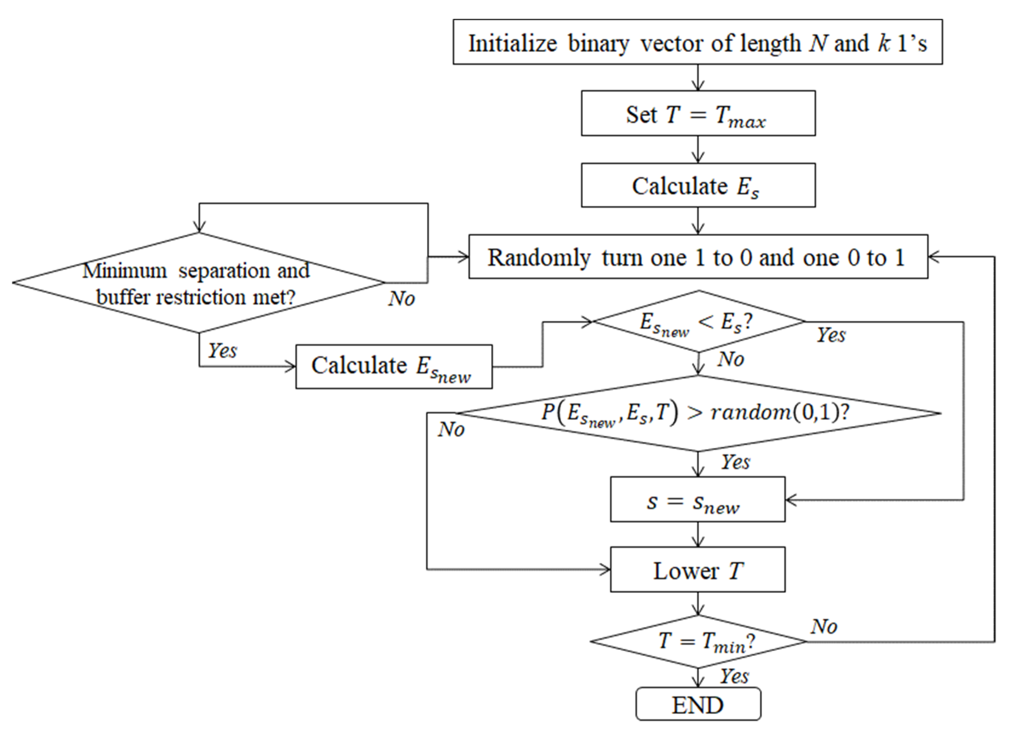
2.2. Simulated Annealing

Rather than sensing the full resolution spectra in each of the three modes, the proposed method uses just a small number of narrow wavelength bands (referred to simply as “wavelengths” in this paper) that are specifically chosen to yield accurate species classifications. Simulated annealing, a heuristic optimization method modeled after the metallurgical annealing process in which the metal undergoes controlled cooling to remove defects and toughen it, was used to select the wavelengths. The simulated annealing algorithm consists of a discrete-time inhomogeneous Markov chain with current state s ( i ) and a cooling schedule defined by a starting temperature, T m a x , a final temperature, T m i n < T m a x , and a total number of steps, n [24]. The goal of the algorithm is to determine the minimum of a user-defined energy function, E ( i ) .
At each iteration i 1 , , n , a new trial state is determined by randomly selecting a “neighbor” of the previous state and calculating its energy. If the resulting energy is less than the energy from the previous iteration, the trial state becomes the new state of the system. If the resulting energy exceeds the energy of the previous energy, the algorithm adopts the trial state with probability given by:
P ( E ( i ) ,   E ( i 1 ) ) = e 1 T ( i ) [ E ( i ) E ( i 1 ) ]
where T ( i ) is the temperature at iteration i . Note that this equation allows the algorithm to occasionally accept states that result in an increase in energy. This can benefit the optimization by preventing it from becoming stuck in local minima. The probability of accepting such states is high at the beginning of the process when the temperature is high but gradually decreases with decreasing temperature. The output of the algorithm is the state with the lowest energy encountered throughout the annealing schedule. Figure 1 provides a summary of this algorithm.
For this wavelength selection problem, we define the state as an array of binary elements indicating the presence or absence of each wavelength in the full-resolution spectrum. Because the collected spectra may contain artifacts at the lowest and highest wavelengths, we institute a fixed buffer of size m at either end of the spectrum. Thus, the state at iteration i can be expressed as
s ( i ) = I ( j )   f o r   j m + 1 , , N m 1
where I ( j ) is 1 to indicate that the jth wavelength is selected and 0 to indicate it is not, and N is the total number of wavelengths in the spectrum. Furthermore, because consecutive wavelengths are highly correlated and thus offer little additional information if both are selected, we institute a minimum separation of q wavelength indices between selected wavelengths. Finally, we set a limit, k , on the number of wavelengths selected such that:
j = m + 1 N m 1 I ( j ) = k
Under these three restrictions, we update the state for each iteration by generating a “neighbor” of the current system state. This is done by randomly de-selecting one wavelength index from the current state and selecting a new one. The energy of the trial state is then calculated as 1 a ( i ) where a ( i ) is the average 4-fold cross validation accuracy (see Section 2.5) as determined using the weighted k-nearest neighbors (WKNN) classifier. WKNN is a variation of the familiar k-nearest neighbors algorithm where the training data points are weighted based on the squared inverse of their distances from the query point. It was chosen as the basis for the energy calculation because of its relatively high classification performance and its rapid training time. Accuracy, in this sense, is calculated as the percentage of correct classifications, weighted by the number of samples per class in the test sets to ensure equal contribution from each class.
The simulated annealing algorithm was implemented in Python 3.7 using the simanneal 0.5.0 library [25]. The temperature parameters were set to T m a x = 25 and T m i n = 0.05 and the number of steps was set to n = 5000 . These temperature values were selected to ensure nearly 100% selection of new states in the initial steps, regardless of whether the energy decreased or increased, and nearly 0% selection of states that increased the energy during the final steps. The number of steps was chosen to balance the desire for rapid processing with the need for algorithm convergence.
We compared the performance of the proposed simulated annealing approach for wavelength selection with three common feature selection methods: analysis of variance (ANOVA), recursive features elimination (RFE), and Extremely Randomized Trees (i.e., Extra Tress) [26] classifier feature importance. The ANOVA method selects features based on their ability to provide separation between the target classes in a linear manner. The RFE method is a standard linear regression method which takes as inputs the desired number of features to select and the linear classification method (in this case, the linear discriminant classifier was used). Finally, the nonlinear Extra Trees method assigns a quantitative importance to each feature based on its relevance to correct classification. Performance comparison was conducted using the same WKNN classifier featured in the simulated annealing algorithm.

2.3. Classification of Fish Species

To evaluate the success of the optimal wavelength selection algorithm, a pair of classification studies were conducted with the goal to determine the correct species of a fillet based on spectral information from a single sample point on the fillet represented by one 10 × 10 pixel block (i.e., voxel). For both studies, a multi-layer perceptron (MLP) neural network served as the primary classifier. In the first study, each spectral mode (i.e., VNIR, fluorescence, and SWIR) was investigated separately and the results of the MLP classifier were compared with results from a collection of common machine learning classifiers. The classifiers were trained on the spectral values from the selected wavelengths and evaluated using 4-fold cross-validation. In the second study, the selected wavelengths from the three spectral modes were combined in the input layer of the MLP classifier, and this spectral fusion method was again evaluated with 4-fold cross-validation. Both studies were repeated for numbers of selected wavelengths k = 3, 4, 5, 6, and 7. Results using all available wavelengths were included as a benchmark for comparison.

2.3.1. Multi-Layer Perceptron (MLP) Classifier

An MLP neural network is a common feed-forward artificial neural network that determines its weight values through supervised learning to yield a nonlinear decision boundary designed to minimize a cost function. In this case, the cost function was defined as the complement of the multiclass classification accuracy (weighted by the number of samples per class). For each of the studies described in the subsequent sections, the same two-layered MLP network shown in Figure 2 was used. To protect against overfitting, dropout with a probability of 50% was applied to both hidden layers [27]. Additionally, L2 kernel regularization (with factor λ = 0.0001) was applied to both hidden layers to protect against overfitting by adding a term to the loss function that increases with the magnitude of the network’s weight vector. The input and hidden layers featured the rectified linear unit (ReLU) activation function, and the output layer included the softmax activation function to yield the classification decision.

2.3.2. Single-Mode Classification Study

In addition to the MLP classifier, four common machine learning classifiers—including support vector machine with a linear kernel (SVM), WKNN, linear discriminant (LD), and Gaussian Naïve Bayes (GNB)—were used to perform classification separately for each of the VNIR, fluorescence, and SWIR data. As with the first study, feature sets consisted of the k spectral samples with no further attempt at feature selection. A 4-fold cross-validation was conducted for each study as a robust estimation of multiclass classification accuracy (weighted by the number of samples per class).
SVM determines the set of maximum-margin hyperplanes to separate the classes in the feature space. WKNN, as explained above, is a variation on the k-nearest neighbors algorithm that weights the training points by the inverse square of their distances from the query point. LD classification makes simplifying assumptions about the data (i.e., Gaussian distributed with the same covariance matrix for all classes) to determine the separating hyperplanes. Finally, GNB combines the probabilities of obtaining the measured value for each input given each specific class and selects the class with the highest resulting probability. GNB assumes statistical independence between the inputs [28]. SVM was included due to its reputation as a high-performance classifier. WKNN, another robust classifier, was included for its performance and because of its use in the simulated annealing algorithm. LD was included for comparison to evaluate any performance degradation that might result from the expected violation of the Gaussian or identical covariance assumptions. GNB was included for comparison to evaluate performance degradation due to the expected violation of independence among the inputs (i.e., the selected wavelengths).
Each classifier was trained with the k = 3, 4, 5, 6, and 7 wavelengths selected by the simulated annealing algorithm for each of the three spectral modes. To place the resulting classification accuracy values in context, the results of this study were compared with benchmark classification accuracies determined using all wavelengths in the full-resolution spectra.

2.3.3. Spectral Fusion Classification Study

For this study, the wavelengths were selected for each of the three spectral modes independently, as discussed in the previous section, and then concatenated into a single vector, which formed a new input layer for the MLP classifier. This classifier was then trained and evaluated (using 4-fold cross-validation) for k = 3, 4, 5, 6, and 7 wavelengths and the results were compared with a benchmark determined by including all wavelengths from the full-resolution spectra. Due to concerns about the usefulness of the SWIR data for species classification, we also evaluated fusion with just the VNIR and fluorescence modes.

2.4. Fish Fillet Data Collection

Figure 3 shows an overview of the data acquisition and processing steps for the studies represented in this paper. The database for this study consisted of VNIR and SWIR reflectance and fluorescence spectra collected from 133 fish fillets representing a total of 25 different species groups (Table 1). The species for each fillet was verified using DNA barcoding [8]. Each fillet was placed in a 150 × 100 × 25 mm sample holder created with a 3D printer (Fortus 250mc, Stratasys, Eden Prairie, MN, USA) using production-grade black thermoplastic. Image acquisition was conducted by the pushbroom method, where a linear motorized translation stage was used to move the sample holder incrementally across the scanning line of the imaging spectrograph. The length of the instantaneous field of view (IFOV) was made slightly longer than the length of the sample holder (150 mm) by adjusting the lens-to-sample distance. The resulting spatial resolution along this dimension was determined as 0.4 mm/pixel. Each fillet was sampled along the width direction (100 mm) of the holder with a step size of 0.4 mm to match the spatial resolution of the length direction [8].
Flat-field corrections were applied to the VNIR and SWIR reflectance images and the fluorescence images to convert the original absolute intensities in CCD counts to relative reflectance and fluorescence intensities [29]. An initial spatial mask was then created for each imaging mode to separate the fish fillets from the background. To filter out inaccurate measurements around the thinner edges and portions of the fillets near the bone structure, an outlier removal scheme was instituted. Outliers were handled by first calculating the mean (μ) and standard deviation (σ) of the fish pixel intensities over the entire fillet. Voxels of 10 × 10 pixels were considered to mimic independent fish fillet spectral point measurements using the field of view of a fiber optic spectrometer. Exclusion occurred if ≥10% of the constituent pixels in a voxel exceeded μ ± 2 σ to eliminate outliers. Figure 4 shows an example result of voxel processing where most of the excluded voxels are concentrated near the fillet edges. This approach produced a final set of spatial masks, one each for the VNIR and SWIR reflectance and fluorescence images, which determined the blocks to be used for analysis. Finally, the fluorescence spectra were scaled by a constant factor of 6000, the approximate maximum of fluorescence spectral values in the database. This was done to set the range of fluorescence values to between zero and one. Alternative normalization methods such as z-score and area under the curve (AUC) normalization were tried as well and produced similar results. However, this simple scaling was chosen because, unlike these alternatives, it requires no knowledge of the entire spectrum and is thus consistent with the concept of collecting only a small number of wavelengths for analysis. Table 1 provides a summary of this database with the numbers of fillets per species and the number of valid voxels for each fillet and each collection mode.
The reflectance and scaled fluorescence spectra for each of the 25 fish species are shown in Figure 5. The significant differences in the shapes and positions of the spectral averages for the various species and the homogeneous nature of the spectra (as indicated by the relatively short error bars) suggest that high classification accuracies can be achieved with this spectral information.

2.5. Cross-Validation Train and Test Datasets

For both the single-mode and the spectral fusion studies, 4-fold cross-validation was conducted by dividing the complete dataset (as described in Table 1) into four disjoint test sets, each of which contained voxels from at least one fillet of each of the 25 species. The corresponding training set for each test set was then composed of all data not in the test set. Four-fold cross-validation (as opposed to the more common 5- or 10-fold versions) was chosen because there was greater variability between fillets of the same species than between voxels of the same fillet. Thus, we wanted to ensure that each test set contained entire fillets that were not included in the corresponding training set. For those species with more than four fillets in the complete dataset (e.g., Malabar blood snapper), the fillets were divided into the four test sets with the goal of having the total number of fillets in each test set as equal as possible.

2.6. Data Imbalance Correction

To prevent classification biases due to data imbalances between the various species, we applied sampling with replacement to each training set to produce 8000 voxel samples per species for a total of 200,000 samples in each training set. No resampling was applied to the test sets, but the measured multiclass classification accuracies were weighted by the number of voxel samples per class to ensure an equal contribution from each species.

3. Results and Discussion

3.1. Wavelength Selection

The purpose of wavelength selection is to enable classification with a limited number of wavelengths (3–7) that can be created using optical filters, LEDs, etc. to produce a simple, low-cost classification device. The robustness of the proposed simulated annealing approach was evaluated by running 10 iterations of the algorithm with the VNIR data for the k = 7 cases and examining the variation in the resulting selected wavelengths and the associated WKNN classification accuracies. Figure 6a shows the wavelengths selected for each of the 10 iterations, with each row of similarly colored dots representing a single iteration. Although some variability in the selected wavelengths is noticeable, the plot of multiclass classification accuracies for these iterations in Figure 6b shows little variability in the resulting accuracy. The standard deviation over these 10 accuracy values was 0.13%.
Figure 7 shows the average VNIR reflectance spectrum for a red snapper fillet with the k = 3, 4, 5, 6, and 7 optimal wavelengths selected by the simulated annealing algorithm. For all k values, the selected wavelengths correspond to interesting peaks, valleys, and inflection points of the spectrum. Clearly, the region of wavelengths <600 nm is favored along with the trough near 950 nm.
The wavelength selections for the fluorescence data in relation to the average spectrum for one of the red snapper fillets are shown in Figure 8. For this mode, the initial wavelength selections are concentrated at the minima of the spectrum with no wavelengths near the large peak around 670 nm selected until the k = 6 case.
Figure 9 shows the wavelength selections for the SWIR reflectance data. The selections for each of the k values are concentrated near the trough around 1000 nm and the inflection point near 1160 nm. No wavelengths above 1200 nm are selected.
Table 2 shows the results of the comparison between the proposed simulated annealing-based wavelength selections method and the three alternative methods. For each combination of spectral mode and number of selected wavelengths, the simulated annealing method yields the set of wavelengths that produces the highest 4-fold cross validated classification accuracy with the WKNN classifier.

3.2. Classification

3.2.1. Results of the Single-Mode Study

Average cross-validated (4-fold) classification accuracies for the VNIR reflectance data are given in Table 3. The column labeled “Benchmark” gives the results for the case where all wavelengths are included. The set of columns under “Selected Wavelengths” list the resulting accuracies based on the spectral values at the k = 3, 4, 5, 6, 7 optimal wavelengths. Results for the fluorescence data are provided in a similar manner in Table 4 and for the SWIR reflectance data in Table 5. Values in bold denote the highest accuracy for each number of selected wavelengths.
Looking first at the accuracies for the benchmark cases, MLP yields the highest accuracy for the fluorescence data but comes in second for the SWIR data and third for the VNIR data. The superior performance of LD, a relatively simple classifier, for the VNIR and SWIR benchmark cases suggests that overfitting is a significant problem for these cases. Accuracies for the SWIR data are far lower, with LD yielding the highest accuracy at just 80.7%. GNB yields the lowest accuracies for all three modes, reinforcing the notion that classification performance is not dependent upon the values from the selected wavelengths themselves but upon their values in relation to one another. The independence assumption of GNB results in low performance.
Looking next at the “Selected Wavelengths” cases, MLP outperforms the other classifiers for all k values and spectral modes (except for the k = 3 case with the VNIR data). Accuracies >85% are possible given spectral values at just seven or fewer wavelengths for the fluorescence data and >80% for the VNIR reflectance data. Most importantly, with MLP trained on only seven spectral values, the resulting accuracies are within 10 percentage points of the benchmark case for all three spectral modes. The highest performance (89.91%) is seen for the fluorescence data.
Figure 10, Figure 11, and Figure 12 show confusion matrices for the k = 7 MLP results from the single-mode VNIR, fluorescence, and SWIR data, respectively. The classification performance is clearly best with the fluorescence data with accuracies >95% for many species. However, the accuracies for some other species are much lower. For example, goosefish has the lowest accuracy at 62.5%, being misclassified as rockfish 28.2% of the time. This is an indication that nearly an entire goosefish fillet was misclassified as rockfish in one of the folds. The overall classification performance is a little lower with the VNIR data. Winter skate shows the lowest classification accuracy at 39.4% in this case, being misclassified as goosefish 26.0% of the time and as almaco jack 13.0% of the time. Much worse performance is seen with the SWIR data, where we find a larger variety of misclassifications. Rockfish has the lowest classification accuracy at just 15.7% with high percentages of misclassification (>14%) as Atlantic cod, haddock, Pacific halibut, and Pacific cod.
The variability of these single-mode classification results with each of the four cross-validation folds can be seen in Figure 13. The lower and upper limits of the error bars in each plot represent the minimum and maximum accuracies, respectively, for the four-folds. The red dashed line in each plot represents the benchmark accuracy obtained by MLP using all wavelengths in the spectrum.
The results of the single-mode classification study prove that high accuracies can be obtained (especially with the MLP classifier) with just seven or fewer wavelengths. The best benchmark performance (92.9%) using all wavelengths was seen with the fluorescence mode with MLP followed by VNIR reflectance (91.7%) and then SWIR reflectance (80.7%), both with LD. The superior performance of LD in these cases suggests the inclusion of all wavelengths significantly increases the potential for overfitting. With seven wavelengths in the fluorescence case, the MLP accuracy came within ~3% of the benchmark accuracy. Review of the confusion matrices from this study reveal that although high overall accuracies can result from these single-mode classifications, each spectroscopic mode has its own unique set of strengths and weaknesses. Furthermore, highly concentrated misclassification results were seen in a few cases, suggesting that entire fillets in the test sets were sometimes misclassified. This is likely a consequence of the somewhat small size of our current dataset. We believe these misclassifications can be alleviated in future studies as we increase the number of fillets per species to better represent the within-species variability of the spectra.

3.2.2. Results of the Fusion Classification Study

Table 6 gives the resulting average 4-fold cross-validation accuracies for the MLP classifier with the spectral modes fused at the input layer. As with the single-mode study, the value in the “Benchmark” column is the accuracy obtained by fusing all wavelengths from the various modes. We present results from the fusion of all three modes as well as results of fusion without the SWIR mode. This latter iteration was included due to the poor performance with the SWIR data in the single-mode study. By fusing the modes, MLP is able to produce classification accuracies that exceed the highest accuracies from the single-mode study by >10% for k = 3 and by >4% at k = 7. An accuracy of >90% is obtained even with only three wavelengths. The fusion accuracies with all three spectral modes exceed the accuracies without the SWIR data only by 1–2 percentage points for the k = 3, 4, 5, 6, 7 cases (and is lower for the benchmark case), indicating that SWIR, in fact, does not contribute independent information for species classification. Figure 14 shows the confusion matrix for the fusion of all three modes with k = 7. Note that although the rates of correct classification are >99% for many species and >90% for 20 species, the large, concentrated misclassification errors seen in the single-mode study were found here as well. Tuna has the lowest classification accuracy at 61.8%, with 27.8% of the misclassifications as Malabar blood snapper. In this case, less than 8% of the voxels from the two tuna fillets in one of the test sets were classified correctly.
These results support the hypothesis that individual strengths of different spectroscopic modes can be combined to form a classifier with superior accuracy. Stated another way, the failure modes of each spectroscopic mode can be mitigated by the other two modes to significantly reduce all misclassification rates. Furthermore, Table 6 and Figure 14 reveal that significant improvements in accuracy are possible even with just three selected wavelengths from each mode. However, the low accuracies found for certain fish species suggest the need for an expansion to the proposed methodology to enable high classification accuracy for large numbers of fish species. We are currently investigating a cascading multiple-model approach that will be the subject of a future publication. Future work with a larger dataset will also include hyperparameter optimization to identify the optimal MLP architectures for each of the single-mode and fusion cases.

4. Conclusions

This effort was designed to evaluate the potential of a new methodology for selecting narrowband wavelengths from multiple spectroscopic modes and combining the spectral values at these wavelengths to enable the accurate classification of materials under investigation. The simulated annealing algorithm was found to robustly produce optimal sets of k wavelengths for k = 3, 4, 5, 6, 7. The results of the two classification studies confirm proof of concept for the proposed methodology to support the design of inexpensive hyperspectral imaging devices to classify fish species featuring homogenous spectral data. Future work will include a larger database of fillets for this same food fraud application and will consider agricultural and biomedical applications where the data is expected to be more heterogeneous. Both the optimization and the classification components of the algorithm will be revised and improved to meet the challenges of these more complex applications.

Author Contributions

J.C.: Methodology, software, formal analysis, writing original draft, visualization, investigation. R.D.: Methodology. K.T.: Review, editing, supervision. A.A., N.M.: Methodology, review, editing. J.Q., D.E.C., C.H., I.B., M.S.K.: Resources, investigation. R.B.I., A.G.Y., J.R., R.S.H.: Data curation. F.V.: Supervision, project administration. All authors have read and agreed to the published version of the manuscript.

Funding

This material is based upon work supported by the National Oceanic and Atmospheric Administration (NOAA) [grant number NA20OAR0210327]. Any opinions, findings, conclusions, or recommendations expressed in this publication are those of the author(s) and do not necessarily reflect the views of NOAA.

Institutional Review Board Statement

Not applicable.

Informed Consent Statement

Not applicable.

Data Availability Statement

Not applicable.

Conflicts of Interest

The authors declare no conflict of interest.

References

  1. Zhu, M.; Huang, D.; Hu, X.-J.; Tong, W.-H.; Han, B.-L.; Tian, J.-P.; Luo, H.-B. Application of hyperspectral technology in detection of agricultural products and food: A Review. Food Sci. Nutr. 2020, 8, 5206–5214. [Google Scholar] [CrossRef]
  2. Lu, Y.; Saeys, W.; Kim, M.; Peng, Y.; Lu, R. Hyperspectral imaging technology for quality and safety evaluation of horticultural products: A review and celebration of the past 20-year progress. Postharvest Biol. Technol. 2020, 170, 111318. [Google Scholar] [CrossRef]
  3. Yuan, D.; Jiang, J.; Qiao, X.; Qi, X.; Wang, W. An application to analyzing and correcting for the effects of irregular topographies on NIR hyperspectral images to improve identification of moldy peanuts. J. Food Eng. 2020, 280, 109915. [Google Scholar] [CrossRef]
  4. Liu, Z.; Jiang, J.; Qiao, X.; Qi, X.; Pan, Y.; Pan, X. Using convolution neural network and hyperspectral image to identify moldy peanut kernels. LWT 2020, 132, 109815. [Google Scholar] [CrossRef]
  5. Sun, J.; Cao, Y.; Zhou, X.; Wu, M.; Sun, Y.; Hu, Y. Detection for lead pollution level of lettuce leaves based on deep belief network combined with hyperspectral image technology. J. Food Saf. 2021, 41, e12866. [Google Scholar] [CrossRef]
  6. Liang, K.; Huang, J.; He, R.; Wang, Q.; Chai, Y.; Shen, M. Comparison of Vis-NIR and SWIR hyperspectral imaging for the non-destructive detection of DON levels in Fusarium head blight wheat kernels and wheat flour. Infrared Phys. Technol. 2020, 106, 103281. [Google Scholar] [CrossRef]
  7. Vasefi, F.; Isaacs, R.; Sokolov, S.; Kang, L.; Hellberg, R.; Farkas, D.L.; Qin, J.; Chan, D.E.; Kim, M.S. Multimode optical imaging for identification of fish fillet substitution and mislabeling (Conference Presentation). In Sensing for Agriculture and Food Quality and Safety XI; International Society for Optics and Photonics: Baltimore, MA, USA, 2019; Volume 11016, p. 1101606. Available online: https://www.spiedigitallibrary.org/conference-proceedings-of-spie/11016/1101606/Multimode-optical-imaging-for-identification-of-fish-fillet-substitution-and/10.1117/12.2523224.short (accessed on 1 January 2021).
  8. Qin, J.; Vasefi, F.; Hellberg, R.S.; Akhbardeh, A.; Isaacs, R.B.; Yilmaz, A.G.; Hwang, C.; Baek, I.; Schmidt, W.F.; Kim, M.S. Detection of fish fillet substitution and mislabeling using multimode hyperspectral imaging techniques. Food Control 2020, 114, 107234. [Google Scholar] [CrossRef]
  9. Goetz, A.F.H. Three decades of hyperspectral remote sensing of the Earth: A personal view. Remote Sens. Environ. 2009, 113, S5–S16. [Google Scholar] [CrossRef]
  10. Kumar, A.; Bharti, V.; Kumar, V.; Kumar, U.; Meena, P.D. Hyperspectral imaging: A potential tool for monitoring crop infestation, crop yield and macronutrient analysis, with special emphasis to Oilseed Brassica. J. Oilseed Brassica 2016, 7, 113–125. [Google Scholar]
  11. Teke, M.; Deveci, H.S.; Haliloğlu, O.; Gürbüz, S.Z.; Sakarya, U. A short survey of hyperspectral remote sensing applications in agriculture. In Proceedings of the 2013 6th International Conference on Recent Advances in Space Technologies (RAST), Istanbul, Turkey, 12–14 June 2013; pp. 171–176. [Google Scholar]
  12. Adão, T.; Hruška, J.; Pádua, L.; Bessa, J.; Peres, E.; Morais, R.; Sousa, J.J. Hyperspectral Imaging: A Review on UAV-Based Sensors, Data Processing and Applications for Agriculture and Forestry. Remote Sens. 2017, 9, 1110. [Google Scholar] [CrossRef] [Green Version]
  13. Benelli, A.; Cevoli, C.; Fabbri, A. In-field hyperspectral imaging: An overview on the ground-based applications in agriculture. J. Agric. Eng. 2020, 51, 129–139. [Google Scholar] [CrossRef]
  14. Wu, D.; Sun, D.-W. Advanced applications of hyperspectral imaging technology for food quality and safety analysis and assessment: A review—Part I: Fundamentals. Innov. Food Sci. Emerg. Technol. 2013, 19, 1–14. [Google Scholar] [CrossRef]
  15. Gat, N. Imaging spectroscopy using tunable filters: A review. In Wavelet Applications VII; International Society for Optics and Photonics: Orlando, FL, USA, 2000; Volume 4056, pp. 50–64. Available online: https://www.spiedigitallibrary.org/conference-proceedings-of-spie/4056/0000/Imaging-spectroscopy-using-tunable-filters-a-review/10.1117/12.381686.short (accessed on 1 January 2021).
  16. Hagen, N.A.; Kudenov, M.W. Review of snapshot spectral imaging technologies. Opt. Eng. 2013, 52, 090901. [Google Scholar] [CrossRef] [Green Version]
  17. Lee, D.J.; Shields, E.A. Compressive hyperspectral imaging using total variation minimization. In Imaging Spectrometry XXII: Applications, Sensors, and Processing; International Society for Optics and Photonics: San Diego, CA, USA, 2018; Volume 10768, p. 1076804. Available online: https://www.spiedigitallibrary.org/conference-proceedings-of-spie/10768/1076804/Compressive-hyperspectral-imaging-using-total-variation-minimization/10.1117/12.2322145.short (accessed on 3 January 2021).
  18. Thompson, J.V.; Bixler, J.N.; Hokr, B.H.; Noojin, G.D.; Scully, M.O.; Yakovlev, V.V. Single-shot chemical detection and identification with compressed hyperspectral Raman imaging. Opt. Lett. 2017, 42, 2169–2172. [Google Scholar] [CrossRef] [PubMed]
  19. Wang, Y.; Lin, L.; Zhao, Q.; Yue, T.; Meng, D.; Leung, Y. Compressive Sensing of Hyperspectral Images via Joint Tensor Tucker Decomposition and Weighted Total Variation Regularization. IEEE Geosci. Remote Sens. Lett. 2017, 14, 2457–2461. [Google Scholar] [CrossRef]
  20. Lee, D.J. Deep neural networks for compressive hyperspectral imaging. In Imaging Spectrometry XXIII: Applications, Sensors, and Processing; International Society for Optics and Photonics: San Diego, CA, USA, 2019; Volume 11130, p. 1113006. Available online: https://www.spiedigitallibrary.org/conference-proceedings-of-spie/11130/1113006/Deep-neural-networks-for-compressive-hyperspectral-imaging/10.1117/12.2528048.short (accessed on 3 January 2021).
  21. Ferrari, C.; Foca, G.; Ulrici, A. Handling large datasets of hyperspectral images: Reducing data size without loss of useful information. Anal. Chim. Acta 2013, 802, 29–39. [Google Scholar] [CrossRef]
  22. Chauvin, J.; Vasefi, F.; Tavakolian, K.; Akhbardeh, A.; MacKinnon, N.; Qin, J.; Chan, D.E.; Kim, M.S. Reconstruction of hyperspectral spectra of fish fillets using multi-wavelength imaging and point spectroscopy. In Sensing for Agriculture and Food Quality and Safety XII; International Society for Optics and Photonics: San Diego, CA, USA, 2020; Volume 11421, p. 114210I, Online only; Available online: https://www.spiedigitallibrary.org/conference-proceedings-of-spie/11421/114210I/Reconstruction-of-hyperspectral-spectra-of-fish-fillets-using-multi-wavelength/10.1117/12.2559230.short (accessed on 14 June 2021).
  23. Kim, M.; Chao, K.; Chan, D.; Jun, W.; Lefcourt, A.; Delwiche, S.; Kang, S.; Lee, K.; Lefcourt, A.; Kang, S.; et al. Line-Scan Hyperspectral Imaging Platform for Agro-Food Safety and Quality Evaluation: System Enhancement and Characterization. Trans. ASABE 2011, 54, 703–711. [Google Scholar] [CrossRef]
  24. Bertsimas, D.; Tsitsiklis, J. Simulated Annealing. Stat. Sci. 1993, 8, 10–15. [Google Scholar] [CrossRef]
  25. Perry, M. Simanneal: Simulated Annealing in Python. Available online: https://github.com/perrygeo/simanneal (accessed on 29 May 2021).
  26. Geurts, P.; Ernst, D.; Wehenkel, L. Extremely randomized trees. Mach. Learn. 2006, 63, 3–42. [Google Scholar] [CrossRef] [Green Version]
  27. Srivastava, N.; Hinton, G.; Krizhevsky, A.; Sutskever, I.; Salakhutdinov, R. Dropout: A Simple Way to Prevent Neural Networks from Overfitting. J. Mach. Learn. Res. 2014, 15, 1929–1958. [Google Scholar]
  28. Hastie, T.; Tibshirani, R.; Friedman, J. The Elements of Statistical Learning: Data Mining, Inference, and Prediction, 2nd ed.; Springer Series in Statistics; Springer: New York, NY, USA, 2009; ISBN 978-0-387-84857-0. Available online: https://www.springer.com/gp/book/9780 (accessed on 8 November 2021).
  29. Kim, M.S.; Chen, Y.R.; Mehl, P.M. Hyperspectral Reflectance and Fluorescence Imaging System for Food Quality and Safety. 2001. Available online: https://pubag.nal.usda.gov/catalog/26654 (accessed on 14 June 2021).
Figure 1. Flowchart for the simulated annealing algorithm used to select the best k wavelength for fish species classification.
Applsci 11 10628 g001
Figure 2. MLP classifier used for the single-band and spectral fusion studies.
Applsci 11 10628 g002
Figure 3. Overview of the data acquisition and processing flow.
Applsci 11 10628 g003
Figure 4. Example of data collection and voxel processing for a red snapper fillet. From the original VNIR image (left), a mask is applied (center) to remove the background and voxels of 10 × 10 pixels are generated (right). Valid voxels are shown in white.
Applsci 11 10628 g004
Figure 5. Average spectra for each of the 25 fish species. (a) VNIR reflectance; (b) scaled fluorescence; (c) SWIR reflectance. Error bars correspond to half of a standard deviation over all voxels for each species.
Applsci 11 10628 g005aApplsci 11 10628 g005bApplsci 11 10628 g005c
Figure 6. Results of the wavelength selection robustness study. (a) Scatter plot showing selected wavelengths for 10 iterations of the k = 7 VNIR study. (b) Plot of final accuracies for each of the 10 iterations.
Applsci 11 10628 g006
Figure 7. Average VNIR reflectance spectrum for one of the red snapper fillets with the optimal k = 3, 4, 5, 6, 7 wavelength selections.
Applsci 11 10628 g007
Figure 8. Average fluorescence spectrum for one of the red snapper fillets with the optimal k = 3, 4, 5, 6, 7 wavelength selections.
Applsci 11 10628 g008
Figure 9. Average SWIR reflectance spectrum for one of the red snapper fillets with the optimal k = 3, 4, 5, 6, 7 wavelength selections.
Applsci 11 10628 g009
Figure 10. Confusion matrix for the single-mode VNIR results with the k = 7 MLP (overall classification accuracy = 82.7%).
Applsci 11 10628 g010
Figure 11. Confusion matrix for the single-mode fluorescence results with the k = 7 MLP (overall classification accuracy = 89.9%).
Applsci 11 10628 g011
Figure 12. Confusion matrix for the single-mode SWIR results with the k = 7 MLP (overall classification accuracy = 67.6%).
Applsci 11 10628 g012
Figure 13. Plot of 4-fold cross-validation accuracies for each of the five classifiers as a function of the number of selected wavelengths in the single-mode classification study for (a) VNIR, (b) fluorescence, and (c) SWIR data. The red dashed line in each plot marks the benchmark accuracy obtained by MLP using all wavelength in the spectrum. Error bars mark the range of accuracies for the four folds.
Applsci 11 10628 g013
Figure 14. Confusion matrix for the fusion of all three spectral modes with k = 7 selected wavelengths (overall classification accuracy = 94.5%).
Applsci 11 10628 g014
Table 1. Fish fillet database summary.
SpeciesNumber of FilletsNumber of Valid Voxels
VNIRFluorescenceSWIR
Almaco Jack (Seriola rivoliana)4115711691992
Atlantic Cod (Gadus morhua)4132213911508
Bigeye Tuna (Thunnus obesus)48315722416
California Flounder (Paralichthys californicus)4101611132416
Char (Salvelinus sp.)4116511561508
Chinook Salmon (Oncorhynchus tshawytscha)4163015702416
Cobia (Rachycentron canadum)4123511701508
Coho Salmon (Oncorhynchus kisutch)48948872416
Gilthead Bream (Sparus aurata)4131412751362
Goosefish (Lophiidae sp.)4130413561508
Haddock (Melanogrammus aeglefinus)4119313751508
Malabar Blood Snapper (Lutjanus malabaricus)12553047507248
Opah (Lampris sp.)49138752416
Pacific Halibut (Hippoglossus stenolepis)4194321202416
Pacific Cod (Gadus macrocephalus)4161917232416
Petrale Sole (Eopsetta jordani)6225324273624
Rainbow Trout (Oncorhynchus mykiss)11426336064806
Red Snapper (Lutjanus campechanus)189482735110,872
Rockfish (Sebastes sp.)4123013102416
Sablefish (Anoplopoma fimbria)49549632416
Sockeye Salmon (Oncorhynchus nerka)410339092416
Swordfish (Xiphias gladius)47897862416
Tuna (Thunnus sp.)6147313143170
Winter Skate (Leucoraja ocellata)4183918151860
Yelloweye Rockfish (Sebastes ruberrimus)4119712162416
Table 2. Results of comparison between wavelength selection methods. Values represent 4-fold cross validation accuracies resulting from training the WKNN classifier with the selected wavelengths.
ModekSimulated AnnealingANOVARFEExtra Trees
VNIR348.23%31.42%27.09%14.09%
457.90%35.20%28.00%23.95%
563.49%36.28%31.87%25.93%
667.08%39.74%37.04%26.62%
768.10%41.21%43.42%29.58%
Fluorescence371.75%59.71%44.18%54.96%
475.90%62.95%48.21%64.09%
577.94%65.83%49.64%63.51%
678.08%66.80%51.95%65.20%
778.27%68.05%58.47%66.30%
SWIR340.15%20.30%15.13%11.56%
446.55%21.20%19.81%17.13%
551.21%37.39%20.15%17.32%
651.77%38.24%30.75%17.39%
752.01%39.26%32.28%16.82%
Table 3. Single-mode classification accuracies (4-fold cross-validation) for the VNIR reflectance data.
BenchmarkSelected Wavelengths
All Wavelengthsk = 3k = 4k = 5k = 6k = 7
MLP87.7%50.4%60.1%72.7%79.7%82.7%
SVM89.8%50.6%59.9%68.7%74.5%77.6%
WKNN69.8%45.6%56.0%61.7%65.1%67.4%
LD91.7%45.0%51.2%54.6%58.4%61.3%
GNB33.1%26.8%31.2%27.3%28.6%31.7%
Table 4. Single-mode classification accuracies (4-fold cross-validation) for the fluorescence data.
BenchmarkSelected Wavelengths
All Wavelengthsk = 3k = 4k = 5k = 6k = 7
MLP92.9%78.9%84.3%86.2%89.4%89.9%
SVM82.5%66.7%71.7%70.8%79.5%79.5%
WKNN79.2%71.1%75.2%77.3%77.1%77.3%
LD84.1%59.0%62.2%65.4%65.5%68.5%
GNB51.0%40.2%45.2%44.0%49.0%49.0%
Table 5. Single-mode classification accuracies (4-fold cross-validation) for the SWIR data.
BenchmarkSelected Wavelengths
All Wavelengthsk = 3k = 4k = 5k = 6k = 7
MLP75.8%46.1%56.1%66.4%67.7%67.6%
SVM63.2%44.5%53.0%62.1%64.2%64.1%
WKNN41.0%38.7%46.3%50.9%52.1%52.6%
LD80.7%38.2%45.2%51.1%53.3%54.5%
GNB20.3%14.4%14.5%14.8%14.7%14.6%
Table 6. Resulting average 4-fold cross-validation accuracies for the fusion of spectral modes in the input layer of the MLP classifier. The values in the “Benchmark” column refer to accuracies obtained using all wavelengths in each spectral mode.
FusionBenchmarkk = 3k = 4k = 5k = 6k = 7
VNIR-Fluor-SWIR94.9%90.4%92.3%93.8%94.8%94.5%
VNIR-Fluor95.5%88.9%90.2%92.4%94.7%94.0%
Publisher’s Note: MDPI stays neutral with regard to jurisdictional claims in published maps and institutional affiliations.

