A Mathematical Model for COVID-19 with Variable Transmissibility and Hospitalizations: A Case Study in Paraguay

Abstract

Forecasting the dynamics of the number of cases with coronavirus disease 2019 (COVID-19) in a given population is a challenging task due to behavioural changes which occur over short periods. Planning of hospital resources and containment measures in the near term require a scenario analysis and the use of predictive models to gain insight into possible outcomes for each scenario. In this paper, we present the SEIR-H epidemiological model for the spread dynamics in a given population and the impact of COVID-19 in the local health system. It was developed as an extension of the classic SEIR model to account for required hospital resources and behavioural changes of the population in response to containment measures. Time-varying parameters such as transmissibility are estimated using Bayesian methods, based on the database of reported cases with a moving time-window strategy. The assessment of the model offers reasonable results with estimated parameters and simulations, reflecting the observed dynamics in Paraguay. The proposed model can be used to simulate future scenarios and possible effects of containment strategies, to guide the public institution response based on the available resources in the local health system.

1. Introduction

Recently, the use of mathematical models in public health decision-making has been increasing, especially to forecast the spread of epidemics [1]. Timely country-based decisions have become critical during the coronavirus disease 2019 (COVID-19) pandemic due to the high contagiousness and the non-negligible proportion of severe cases [2,3]. After a year of intensive research, several types of vaccines for COVID-19 were developed and approved, but are not widely available in most of the countries [4]. Thus, the use of mathematical models in forecasting the course of this pandemic and the required hospital resources is still relevant in order to enforce measures to maintain the situation at levels that can be sustained by a local health system.

A vast amount of works use mathematical models to study the dynamics of the spread of COVID-19 in different contexts [5,6,7,8,9,10,11,12,13,14]. The dynamics of epidemic transmission can be represented by compartmental models based on a system of ordinary differential equations [15]. In these models, the population in a region is divided into groups or compartments such as susceptible, exposed, infectious, recovered, among others, where other groups can be added and/or removed depending on the dynamics or mechanism to be modelled.

Among the simplest and most traditional models for the dynamics of transmission of COVID-19, we find the Susceptible–Infectious–Recovered (SIR) model and, the Susceptible–Exposed–Infectious–Recovered (SEIR) model. Cooper et al. [5] have presented modifications of the SIR model by considering variable the susceptible population, and Ellison [6] have added heterogeneity to the population. Further modifications of the model can be seen in the work of Crokidakis [7], who has included a “quarantined” group in order to analyse the effect of isolation of newly confirmed cases. Additionally, He et al. [8], based on the SEIR model, proposed to divide the infected group into two groups, being with and without interventions, and have also incorporated the “quarantined” and hospitalised groups.

On the other hand, Arino and Portet [11] have considered the latently infected and asymptomatic infectious groups in order to take into account the pre-symptomatic or asymptomatic transmission, which are characteristics of the COVID-19 [9,10]. Additionally, they have subdivided each group into stages to incorporate the Erlang distribution of residence times in each group [16]. There are more elaborate models, such as, SIDARTHE proposed in [12] or $\mathit{\theta }$-SEIHQRD presented in [13], where more compartments are included. In metapopulation models, the spread dynamic of disease is split into age groups or regions, and these groups are interconnected to each other by additional interaction or mobility terms. For instance, Arenas et al. [14] applied a metapopulation model with age-stratified and mobility-based for the spread of COVID-19.

Although there have been published several works proposing mathematical models for the spread dynamics of COVID-19, there are still challenges in adapting particular models in specific situations. These challenges are related to:

• the amount of available data and the quality of such data, that vary from one country to another, and 
• the containment strategies applied in each country.

In particular, highly detailed models are composed of many parameters, which have to be determined independently, using different groups of data. When the available data is limited, then the models with many parameters are over-fitted, which increases the prediction error [17]. However, the simple SIR or SEIR models with constant parameters along the epidemic cycle, fail to represent the dynamics when different containment strategies are applied along the time.

Thus, we developed a mathematical model, which is as simple as possible, but at the same time, applicable to several situations. Our model, named SEIR-H, is based on the simple SEIR model, where R stands for reported instead of recovered. The reported group is composed of individuals who have been diagnosed as positive confirmed cases. Also, in order to answer the specific question about required hospital resources, our model tracks the number of hospitalisations and admissions to an Intensive Care Unit (ICU) of COVID-19 patients. Some parameters, such as the latent period or the average residence times in each compartment or group, are maintained constants as in traditional SEIR models. A key feature that distinguishes our model is to allow the transmissibility and proportions of individuals who need hospital beds or ICU, to vary daily with a moving time-window strategy.

Most of the mathematical models developed in the context of the COVID-19 pandemic were applied to large countries or those with early outbreaks, with a large amount of available data. However, in the context of limited data availability in low-to-middle-income countries, specific models and strategies are needed to overcome this difficulty. In particular, the mathematical model developed in this work is based on limited data available from Paraguay, where except around the capital city, there is no regular testing policy in the rest of the country, nor a good record of region-based mobility. The data used in order to calibrate the model was provided by the Ministry of Public Health and Social Welfare (MSPyBS: Ministerio de Salud Pública y Bienestar Social) and Health Monitoring Centre in Paraguay (DGVS: Dirección General de Vigilancia de la Salud) (http://dgvs.mspbs.gov.py/, accessed on 20 May 2021).

The spread of COVID-19 in Paraguay is characterised by a strongly enforced initial lockdown, which kept the amount of new positive cases low for several months. In this sense, it is worth discussing the effect of early lockdown in the dynamics of spread, as well as, how the time-varying parameters can explain different scenarios observed in Paraguay. The feature of time-varying parameters allows a user to draw future scenarios and use our model as a prediction tool to guide decision-making to contain outbreaks and plan hospital resources accordingly.

The work is organised as follows: the proposed model is presented in Section 2 including the spread dynamics in Section 2.1.1 and the dynamics of hospital resources in Section 2.1.3, as well as the parameter estimations in Section 2.3; Section 3 shows the results obtained and the forecast capability of the model, and it is followed by the discussions in Section 4, the relevance of the present work in Section 5, and final remarks in Section 6.

2. Materials and Methods

In this section, a description of the SEIR-H model is given in Section 2.1. Section 2.2 gives a brief overview of the restriction policies applied in Paraguay. Finally, the methodology used for parameter estimation is presented in Section 2.3.

2.1. SEIR-H Model

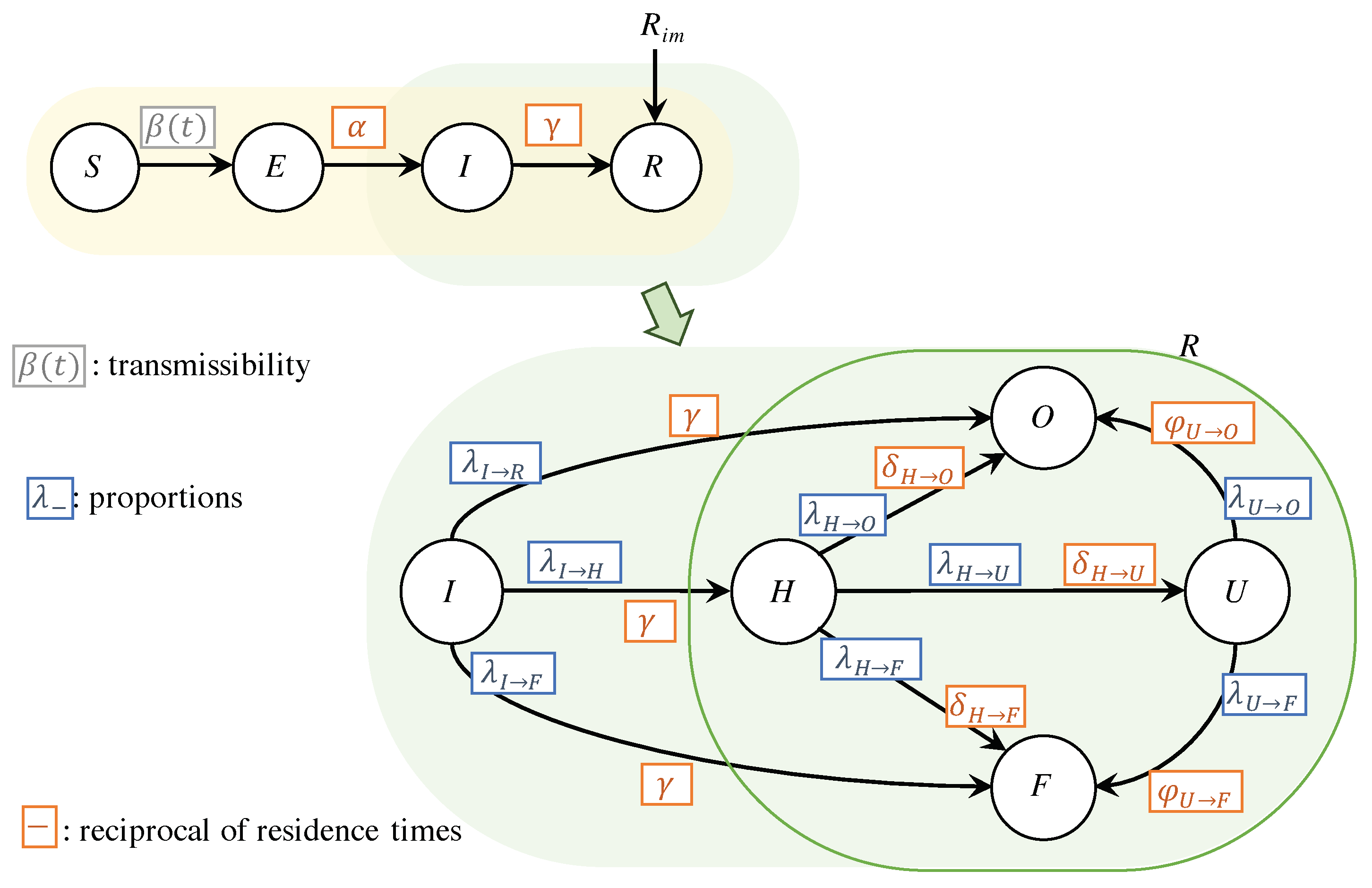
The SEIR-H model is a compartmental model. For the COVID-19 spread dynamics, the SEIR-H model is nearly identical to the classic SEIR model, with the difference that in the proposed model, the group R stands for the reported individuals, who are diagnosed as confirmed positive cases. This reported group is split mainly into three groups: (i) H: hospitalised group, composed of individuals who have severe symptoms, and thus are hospitalised, (ii) U: a group composed of individuals who are admitted to ICU due to the worsening of the symptoms, and (iii) F: death. Thus, the SEIR-H model is separated into two parts representing two dynamics: (i) the dynamics of spread/transmission of the disease, and (ii) the dynamics of the use of hospital beds. In this model, the dynamics of hospital resources do not affect the spread dynamics of the disease, i.e., the compartments S, E, I, R are not influenced by H, U and F. This assumption is reasonable in the sense that the disease transmissions from the hospitalised COVID-19 patients are negligible compared to the transmissions occurring in the community outside the hospitals.

Figure 1 schematically illustrates the proposed SEIR-H model. Both parts of the model are highlighted: (i) the spread dynamics with yellow background, (ii) the dynamics of reported cases in green background. The parameters in blue are associated with the proportions of individuals moving from one compartment to the next, and the parameters in orange are associated with the reciprocal of the average length of stay in each compartment. In the next subsections, both parts are discussed in detail by presenting the systems of differential equations along with the definitions of the parameters. The compartment O in Figure 1, corresponds to those who are recovered from COVID-19. In this work, we do not track the count of recovered individuals, because the data of those recovered are unreliable. Thus, the equation for this compartment is omitted.

2.1.1. Dynamics of The Spread

The spread dynamics of the disease, highlighted in yellow in Figure 1, is similar to the SEIR model [15], and is given by:

$$\begin{array}{cc}\hfill {\displaystyle \frac{dS}{dt}}& =-\beta {\displaystyle \frac{S}{N}}I,\hfill \end{array}$$

(1)

$$\begin{array}{cc}\hfill {\displaystyle \frac{dE}{dt}}& =\beta {\displaystyle \frac{S}{N}}I-\alpha E,\hfill \end{array}$$

(2)

$$\begin{array}{cc}\hfill {\displaystyle \frac{dI}{dt}}& =\alpha E-\gamma I,\hfill \end{array}$$

(3)

$$\begin{array}{cc}\hfill {\displaystyle \frac{dR}{dt}}& =\gamma I+R_{im}.\hfill \end{array}$$

(4)

In this model, the Equations (1)–(4), respectively, show the dynamics of the compartments of: the susceptible S, the exposed E, the infectious I and the reported R. The term $R_{im}$ represents a rate of reported cases from the travellers, which was relevant at the beginning of the dynamics of COVID-19 in Paraguay. The susceptible group S represents those who have not yet contracted the disease and could contract it in the future.

The exposed group E represents those who were exposed to the infection and have been infected, but are in a latent period not yet capable of infecting others. The latent period refers to the time between exposure to the virus and the moment when the individual becomes contagious and is one of the epidemiological characteristics of COVID-19 [8,18,19,20,21] While in the classic SEIR model, compartment E could include those in the incubation period [22], in this work, however, we only include in E those in the latent period. It is crucial to establish this distinction between the latent period and the incubation period, since COVID-19 is characterised by a pre-symptomatic infection [9,10,23]. Furthermore, the inclusion of the E-compartment can resemble the Erlang distribution in the infectious period [11].

The infectious compartment I represents individuals who become contagious. The key feature which distinguishes compartments I from E, is the onset of infectivity. Individuals in I may transmit the disease to susceptibles in S, even without presenting symptoms.

The compartment R is composed of those who are reported with the confirmation of COVID-19 positive diagnosis. In the classic SEIR model, the R compartment is associated with those who are recovered or removed from the dynamics after a certain time. In this work, the R compartment also has the meaning of removed, given the assumption that those who are reported are also isolated and removed from the transmission dynamics. However, since R will be fitted to the officially positive confirmations, we rename it as the reported compartment. The population N is maintained constant throughout the time, equal to the initial population. This condition differs from the actual population that varies due to the reported cases from the travellers $R_{im}$, and also because of the individuals who are travelling abroad (which are not considered in the proposed model).

Three parameters appear in this model: (i) $\beta \left(t\right)$ is the rate at which susceptible individuals acquire the disease, also known as transmissibility, which is time-dependent in this work, (ii) $\alpha$ is the rate at which an exposed individual becomes infectious, also defined as the reciprocal of the average latent period, and (iii) $\gamma$ is the rate at which an infectious individual is reported, expressed as the reciprocal of the average time an individual remains contagious to other individuals.

Table 1. SEIR-H parameters.

Parameter	Description	Type *	Value **
$\beta$	Transmissibility.	T-D	Est.
$\alpha$	Reciprocal of average latent period.	C	1/3 ${}^{\left(a\right)}$
$\gamma$	Reciprocal of average infectious period.	C	1/7 ${}^{\left(b\right)}$
${\lambda }_{I\to H}$	Proportion of infected that are hospitalised.	T-D	Est.
${\lambda }_{I\to F}$	Proportion of infected that are death.	T-D	Est.
${\lambda }_{H\to U}$	Proportion of hospitalised that are admitted in ICU.	T-D	Est.
${\lambda }_{H\to F}$	Proportion of hospitalised that are death.	T-D	Est.
${\lambda }_{U\to F}$	Proportion of admitted in ICU that are death.	T-D	Est.
${\delta }_{H\to U}$	Reciprocal of average stay in hospitals bed before admittion in ICU.	C	1/7 ${}^{\left(c\right)}$
${\delta }_{H\to F}$	Reciprocal of average stay in hospital bed before death.	C	1/9 ${}^{\left(c\right)}$
${\delta }_{H\to O}$	Reciprocal of average recovery period in hospital bed.	C	1/11 ${}^{\left(c\right)}$
${\phi }_{U\to F}$	Reciprocal of average stay in ICU before death.	C	1/11 ${}^{\left(c\right)}$
${\phi }_{U\to O}$	Reciprocal of average recovery period in ICU.	C	1/12 ${}^{\left(c\right)}$

* T-D: Time-Dependent; C: Constant. ** Est.: indicates that the values will be estimated using the methodology described in Section 2.3; all periods of time in this table are considered in days. ${}^{\left(a\right)}$ See [18,19,20,21,24,25]. ${}^{\left(b\right)}$ See [18,20,25,26]. ${}^{\left(c\right)}$ Obtained from the data provided by DGVS.

shows the parameters of the SEIR-H model, with its descriptions and values, and whether it is considered to be constant or time-dependent.

2.1.2. Reproduction Number

The dynamics of disease transmission can be expressed using a single parameter called the reproduction number $R_0$. This number can be defined as the expected number of secondary cases that arise after introducing an infectious individual into a susceptible population. This reproduction number is useful to define a threshold value to be maintained for a certain time, for the epidemic to persist ($R_0>1$), or be extinguished ($R_0<1$) [15,27,28].

The reproduction number is affected by various biological, socio-behavioural and environmental factors [27]. The numerical value depends on the estimation method, and the specific value obtained from the mathematical models based on differential equations should be understood as a threshold rather than as the number of secondary cases [28]. The numerical value can be considered a function of three parameters: the duration of the infectious period, the average probability of transmission of the virus in each contact and the average rate of contacts [27].

The reproduction number of the classic SEIR model can be expressed in terms of the parameters $\beta$ and $\gamma$, as follows:

$$R_0={\displaystyle \frac{\beta }{\gamma }}.$$

(5)

As the spread of disease is evolving, the number of susceptible individuals declines monotonically. Thus, the number in which effectively works as an epidemic threshold is:

$$R_e\left(t\right)={\displaystyle \frac{\beta \left(t\right)}{\gamma }}{\displaystyle \frac{S\left(t\right)}{N}},$$

(6)

also known as the effective reproduction number. This expression is obtained by adding the right-hand sides of the Equations (2) and (3) and then making it equal to zero.

From these equations, it can be observed that the value of the reproduction number $R_0$ or $R_e\left(t\right)$ can be altered by interventions on parameters $\beta$ and $\gamma$. Containment and social distancing measures can affect the parameter $\beta$, by reducing the average rate of contacts. However, hygiene recommendations and proper use of face masks can also affect $\beta$ by reducing the average probability of virus transmission in each contact. While the parameter $\gamma$ depends on the disease itself, it can be altered by effective tracing, testing and isolation of infected individuals.

2.1.3. Dynamics of Required Hospital Resources

The dynamics of reported cases, highlighted in green in Figure 1, is mainly focused on the number of reported individuals in need of general hospitalisations and Intensive Care Units (ICUs). Hence, it is important to analyse the portion of infected individuals that develop severe cases of the disease as well as the fatality rate.

A compartmental model is considered: (i) the compartment H includes general hospitalisation of COVID-19 patients, (ii) the compartment U includes all those reported individuals requiring ICU, and (iii) the compartment of the deceased F. In this work, we use the letter F for the deceased because it is the first letter of the translation in Spanish of the deceased (Fallecido).

The equations that describe the dynamics in hospitals can be expressed as follows:

$$\begin{array}{cc}\hfill {\displaystyle \frac{dH}{dt}}& ={\lambda }_{I\to H}\gamma I-{\lambda }_{H\to U}{\delta }_{H\to U}H-{\lambda }_{H\to F}{\delta }_{H\to F}H-{\lambda }_{H\to O}{\delta }_{H\to O}H,\hfill \end{array}$$

(7)

$$\begin{array}{cc}\hfill {\displaystyle \frac{dU}{dt}}& ={\lambda }_{H\to U}{\delta }_{H\to U}H-{\lambda }_{U\to F}{\phi }_{U\to F}U-{\lambda }_{U\to O}{\phi }_{U\to O}U,\hfill \end{array}$$

(8)

$$\begin{array}{cc}\hfill {\displaystyle \frac{dF}{dt}}& ={\lambda }_{I\to F}\gamma I+{\lambda }_{H\to F}{\delta }_{H\to F}H+{\lambda }_{U\to F}{\phi }_{U\to F}U.\hfill \end{array}$$

(9)

The dynamics of the portion of infected individuals who develop severe cases and need to be hospitalised, is represented in Equation (7), by using a parameter ${\lambda }_{I\to H}$. A portion of those who are hospitalised, given by the parameter ${\lambda }_{H\to U}$, require intensive care. The average length of stay at a normal bed before requiring an intensive care unit, is given by $1/{\delta }_{H\to U}$. However, hospitalised individuals are dying with portion ${\lambda }_{H\to F}$ with average staying in a hospital of $1/{\delta }_{H\to F}$. The rest of the portion ${\lambda }_{H\to O}=1-{\lambda }_{H\to U}-{\lambda }_{H\to F}$ is recovered with average staying in hospital of $1/{\delta }_{H\to O}$.

The Equation (8) represents the dynamics of the occupation of ICU. The admission in ICU is restricted to individuals with severe cases who are initially hospitalised in normal beds. The portion of dying individuals from the ICU is ${\lambda }_{U\to F}$, with an average stay in ICU of $1/{\phi }_{U\to F}$. The recovered portion is ${\lambda }_{U\to O}=1-{\lambda }_{U\to F}$, with average stay in ICU of $1/{\phi }_{U\to O}$.

The last compartment corresponds to accumulated death, given by the Equation (9). Here, it is included those who die from those hospitalised and also those who were in ICU. In addition, a certain portion given by ${\lambda }_{I\to F}$ dies without admission in the hospitals.

2.2. Containment Measures in Paraguay

The first confirmed COVID-19 positive case in Paraguay was reported on 7 March 2020 (First case of the new coronavirus in Paraguay: https://www.mspbs.gov.py/portal/20535/primer-caso-del-nuevo-coronavirus-en-el-paraguay.html, accessed on 20 May 2021). Before the COVID-19 pandemic has reached Paraguay, the country was emerging from one of the worst dengue fever epidemics (The worst Dengue epidemic has been contained: https://www.mspbs.gov.py/portal/20525/la-peor-epidemia-de-dengue-esta-contenida.html, accessed on 20 May 2021). Thus, the government had adopted very strong containment policies in order to gain some time to strengthen the health system (Gs. 530 billion in supplies and 2700 health contracts: https://www.mspbs.gov.py/portal/20576/g-530-mil-millones-en-insumos-y-2700-contratos-para-salud.html, accessed on 20 May 2021; Personal protective equipment delivered to health regions: https://www.mspbs.gov.py/portal/20621/entregan-equipos-de-proteccion-personal-a-regiones-sanitarias.html, accessed on 20 May 2021). This lockdown lasted at least two months, after which the government adopted a system of gradual lifting of the containment measures with enumerated phases: from the most rigorous confinement at Phase 0 to the more relaxed at Phase 4. After that, the policy named “New normality” is applied, which is the most relaxed measure with specific restrictions in certain areas depending on its situation.

Table 2. Quarantine phases during the COVID-19 pandemic in Paraguay, until May 2021 [29,30].

Denomination	Time Frame	Description
Pre-quarantine	11 March to 19 March 2020	- Curfew from 8 p.m. to 4 a.m. - First restrictions taken.
Phase 0	20 March to 3 May 2020	- 24 h curfew. - Confinement/isolation.
Phase 1	4 May to 24 May 2020	- Curfew from 9 p.m. to 5 a.m. - Flexibility: marginal.
Phase 2	25 May to 14 June 2020	- Curfew from 9 p.m. to 5 a.m. - Flexibility: slight.
Phase 3	15 June to 19 July 2020	- Curfew from 23 p.m. to 5 a.m. (Sunday to Thursday) and midnight to 5 a.m. (Friday to Saturday). - Flexibility: moderate. - Greater local restrictions in two departments, representing at most 7% of the population.
Phase 4	20 July to 4 October 2020	- Curfew from 23 p.m. to 5 a.m. (Sunday to Thursday) andmidnight to 5 a.m. (Friday to Saturday). - Flexibility: high. - Greater local restrictions in six departments, representing at most 61% of the population.
New normality	From 5 October 2020	- Curfew from midnight to 5 a.m. (but from 8 p.m. to 5 a.m. in red areas). - Only specific restrictions, until the appearance of the vaccine or cure.

summarise the different phases of quarantine (while the term quarantine is used for mobility restrictions on exposed individuals, in Paraguay, this term is widely adopted to refer to the various degrees of lockdown measures) in Paraguay. Local and temporary restrictions that differ from the main phases can be consulted in Appendix A.

2.3. Estimation of Model Parameters

This section presents the methodology to estimate the parameters of the proposed model. For this purpose, we use data provided by the Ministry of Public Health and Social Welfare, and the Health Monitoring Centre. The available data are daily records of:

1.

diagnosed with positive confirmed cases or daily reported cases $D^R\left(t_j\right)$, excluding the count of confirmed cases from travellers,

2.

diagnosed with positive confirmed cases in the isolated groups who were travellers from abroad $R_{im}\left(t_j\right)$,

3.

occupation in general bed in the hospitals by the patients of COVID-19 $D^H\left(t_j\right)$,

4.

occupation in ICU by patients of COVID-19 $D^U\left(t_j\right)$,

5.

confirmed daily deaths by COVID-19 $D^F\left(t_j\right)$.

These data in a specific day are assumed to be independent of each other. These data are from $t_1=$ 7 March 2020 until $t_{j_{\mathrm{end}}}=$ 22 May 2021. From the data provided by the Health Monitoring Centre, it was determined: (i) the average time of stay in general beds in the hospitals by the COVID-19 patients, and (ii) the average time of ICU stay by COVID-19 patients.

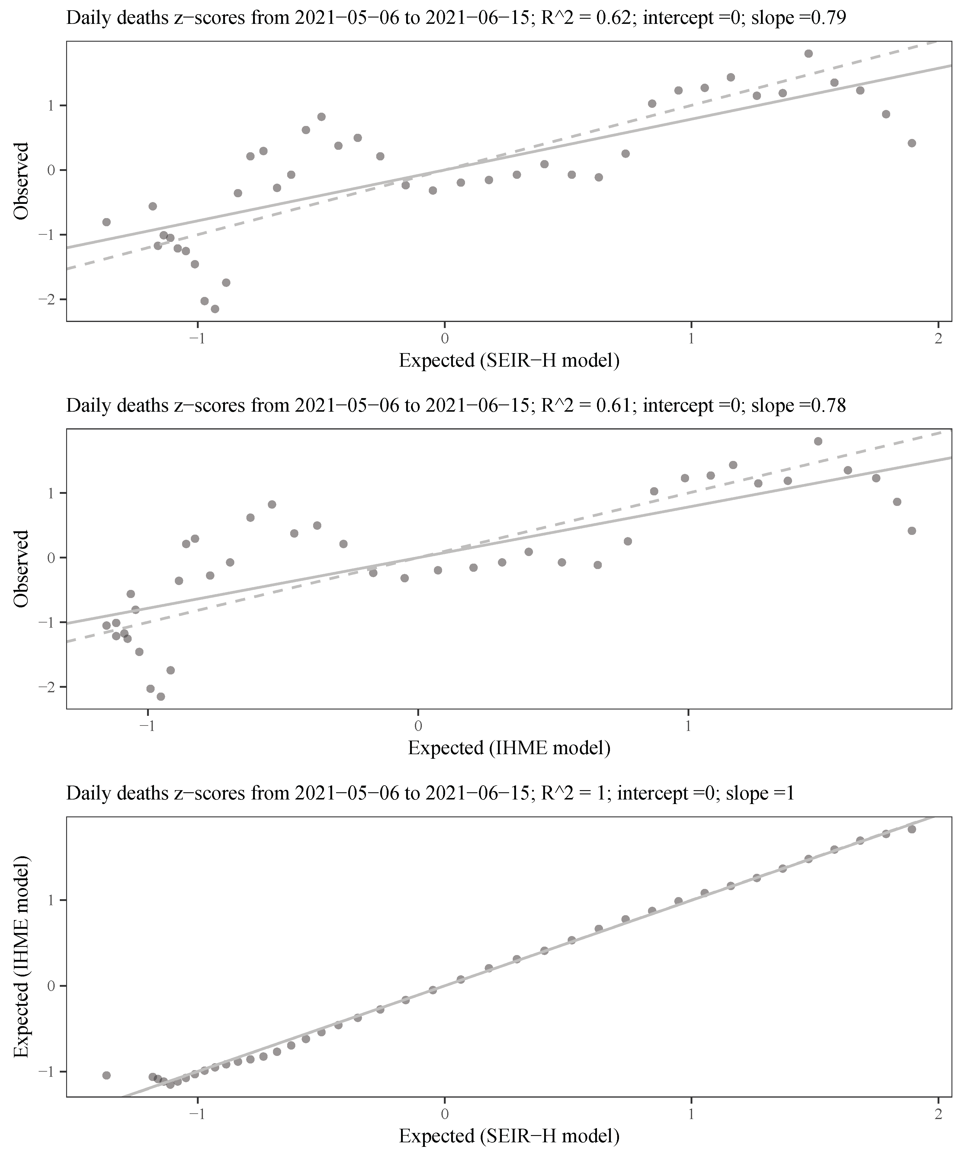
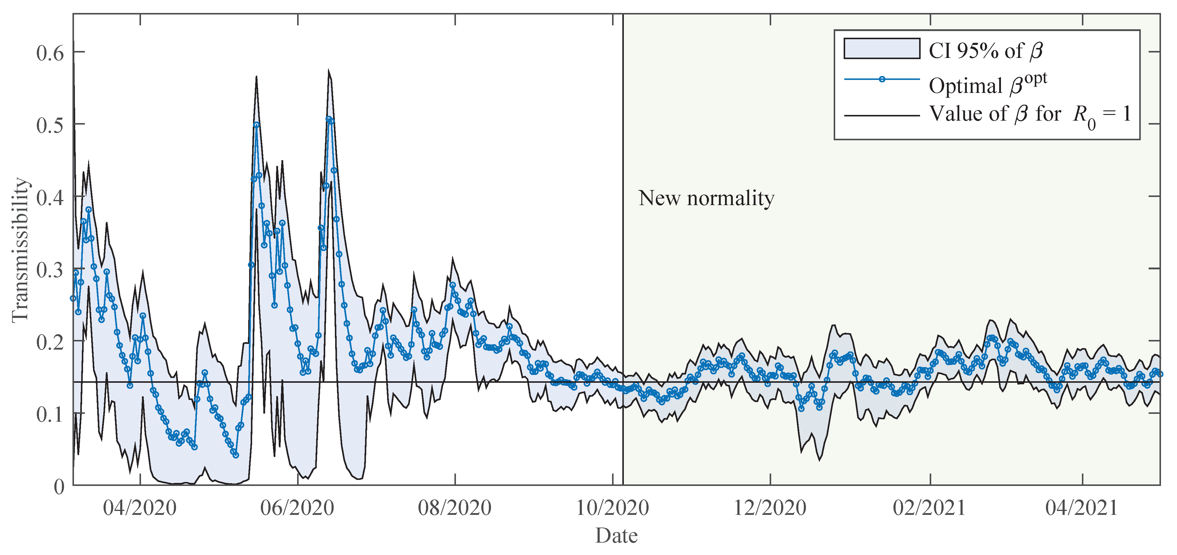
The estimation of the model parameters is mainly performed in two steps: (i) the estimation of the transmissibility $\beta$ of the disease for the spread dynamics using the Equations (1)–(4), and (ii) the different portions ${\lambda }_{*}$, with $*\in \{I\to H,I\to F,H\to U,H\to F,U\to F\}$, for bed occupations in hospitals using the Equations (7)–(9) in addition with the Equations (1)–(4). The estimation of transmissibility $\beta$ is performed from the date of the first confirmed positive case in Paraguay, at $t_1$. Due to the initial strong containment, the amount of hospital bed occupations by COVID-19 patients remained very low for several months.

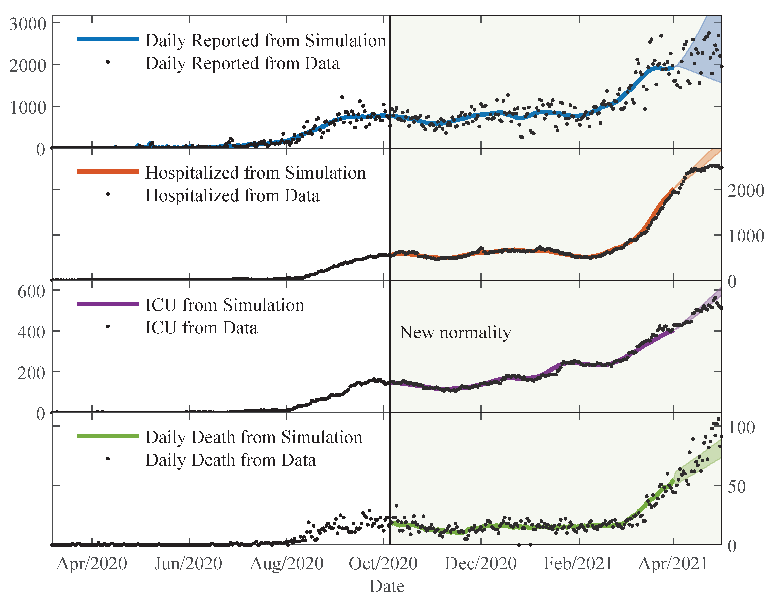
Because of this conditions, and due to the high intermittency of the available data, there were difficulties in estimating the portions ${\lambda }_{*}$, thus these values are estimated only as of $t_{j_h}=$ 5 October 2020, when the “new normality” policy measures are applied. Consequently, the states of H, U and F, which are associated with these proportions are simulated from $t_{j_h}$.

The time-varying parameters are determined using the moving time-window. In this work, we fixed the size of the time-window to $W=14$ days. In the classic SEIR model, the time-window size would correspond to the entire epidemic cycle, keeping the transmissibility $\beta$ invariant over the cycle. This hypothesis is a reasonable assumption in seasonal flu epidemics, because most of the population do not change their behaviour during the season. However, this condition is not the case with the COVID-19 pandemic, because behavioural changes of the population are continuous and vary mainly in response to official containment measures. Thus, in order to capture the relevant dynamics of transmission, a mechanism is needed to approach a time-varying transmissibility.

The strategy of using a moving time-window in the parameter estimation resembles the moving average for time-series data, i.e., a smaller time-window size will better fit daily noisy data with higher oscillations, and on the other hand, a larger time-window size will offer smoother results and reveal trends. Thus, parameters obtained using time-windows with size $W=14$ days can be understood as an average during this time span. This size was chosen mainly because of two reasons: (i) according to the officials at the Health Monitoring Centre in Paraguay (DGVS), the delay from the day when a contagion occurs until the detection is normally at least 10 days, and (ii) the strategy of containment measures in Paraguay is usually dictated in a two-week time span.

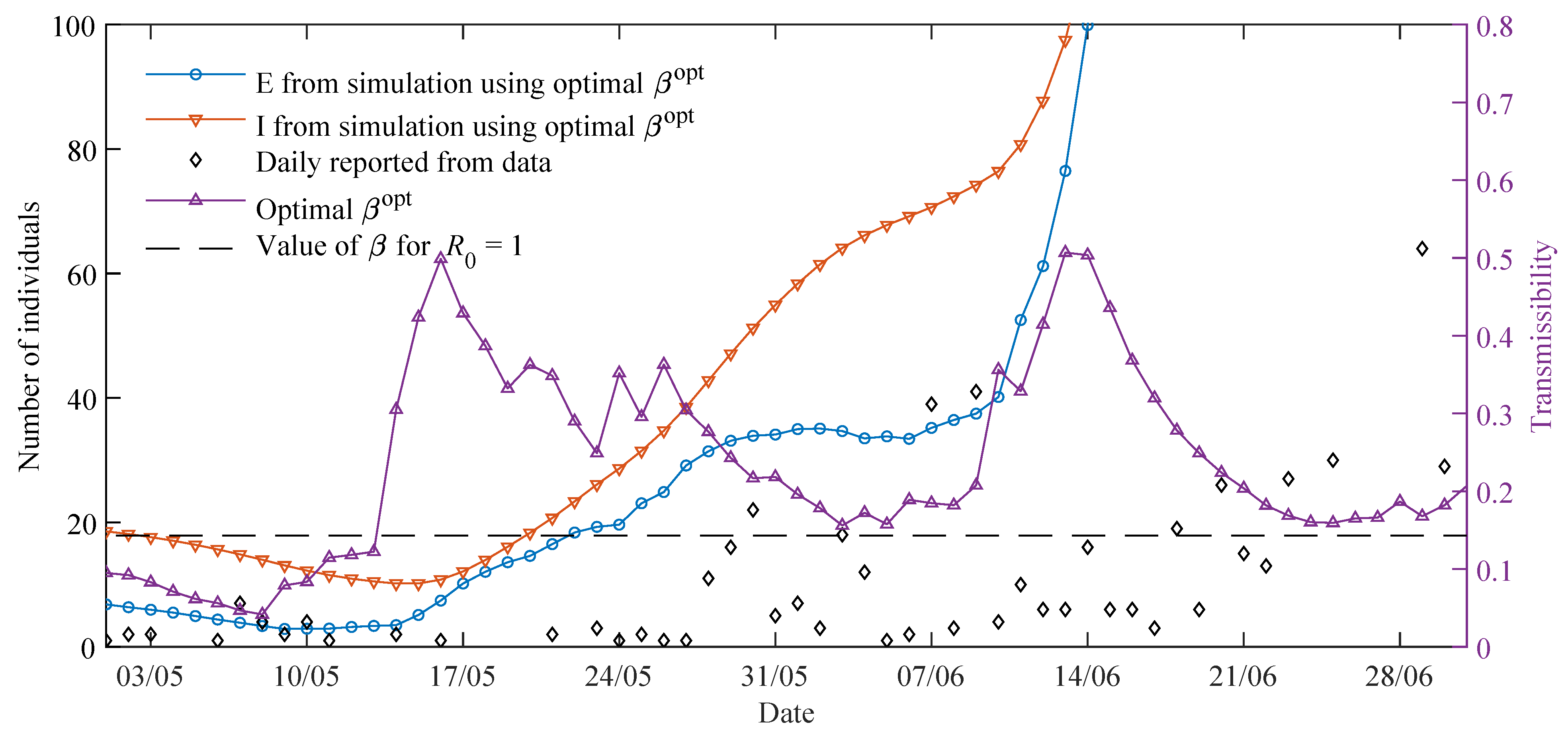
Algorithm 1 shows schematically the procedure for parameter estimation. The required information is the set of parameters which are maintained constant (see Table 1), the data $D^R\left(t_j\right)$, $D^H\left(t_j\right)$, $D^U\left(t_j\right)$, $D^F\left(t_j\right)$, $R_{im}\left(t_j\right)$, from $j=1$ to $j=j_{\mathrm{end}}$, population N and size of time-window W. The results are the transmissibility $\beta \left(t_j\right)$ from $j=0$ to $j=j_{\mathrm{end}}-W$, and the proportions ${\lambda }_{*}\left(t_j\right)$ from $j=j_h$ to $j=j_{\mathrm{end}}-W$.

Algorithm 1: Parameter estimation

2.3.1. Estimation of Initial Condition

The population of Paraguay is estimated at $N=7,252,671$ according to the National Institute of Statistics (INE: Instituto Nacional de Estadística https://www.ine.gov.py/default.php?publicacion=2, accessed on 20 May 2021). The initial time is set on $t_0=6\mathrm{March}2020$, one day before the day when the first case is reported. On this day, the reported group is set as $R\left(t_0\right)=0$, and the initial conditions for: the exposed $e_0=E\left(t_0\right)$, the infectious $i_0=I\left(t_0\right)$ and the transmissibility $\beta \left(t_0\right)$ are estimated using $D_0^R=\left\{D^R(t_0+k)\right|k=1,\dots ,W\}$, available data of daily reported or confirmed cases in the first $W=14$ days (Algorithm 1, line 1). The initial susceptible population is $S\left(t_0\right)=N-E\left(t_0\right)-I\left(t_0\right)-R\left(t_0\right)$.

Some parameters that do not depend on the particularities of each country or region but on the disease itself are set according to the values presented in the literature. The average of the latent period is $1/\alpha =3$ days [18,19,20,21,24,25] and the average of the infectious period is $1/\gamma =7$ days [18,20,25,26] (see Table 1). Although the infectious period can be reduced by early tracing and isolation (quarantine) strategies for infectious persons, after the movement restriction period and throughout much of the pandemic in Paraguay, early tracing and isolation of infectious persons was difficult.

The estimation is performed using the Bayesian method, which can be expressed as:

$$P(e_0,i_0,{\beta }_0,{\sigma }_0^R|D_0^R)\propto P\left(D_0^R\right|e_0,i_0,{\beta }_0,{\sigma }_0^R)P(e_0,i_0,{\beta }_0,{\sigma }_0^R),$$

(10)

where $P(e_0,i_0,{\beta }_0,{\sigma }_0^R|D_0^R)$ is the posterior probability distribution of the parameters $\{e_0$, $i_0$, ${\beta }_0$, ${\sigma }_0^R\}$ given the observation of the data $D_0^R$, $P\left(D_0^R\right|e_0,i_0,{\beta }_0,{\sigma }_0^R)$ is the probability of observing the data $D_0^R$ given specific values of the parameters, which is also known as likelihood function, and $P(e_0,i_0,{\beta }_0,{\sigma }_0^R)$ is the prior probability distribution of the parameters.

We assumed that the observed data $D_0^R$ are normal-distributed around the daily reported cases $d{R}^{e_0,i_0,{\beta }_0}$ from the simulations results using the parameter set $\{e_0,i_0,{\beta }_0\}$ with standard deviation ${\sigma }_0^R$. Thus, the likelihood function can be expressed as:

$$P\left(D_0^R\right|e_0,i_0,{\beta }_0,{\sigma }_0^R)=\prod _{k=1}^W{\displaystyle \frac{1}{\sqrt{2\pi }{\sigma }_0^R}}\exp \left[{\displaystyle \frac{{\left(D^R(t_0+k)-d{R}^{e_0,i_0,{\beta }_0}\left(t_k\right)\right)}^2}{2{\left({\sigma }_0^R\right)}^2}}\right],$$

(11)

where given a set of values of the parameters $\{e_0,i_0,{\beta }_0\}$, the simulated daily reported cases $d{R}^{e_0,i_0,{\beta }_0}$ are obtained by:

$$d{R}^{e_0,i_0,{\beta }_0}\left(t_k\right)=R^{e_0,i_0,{\beta }_0}\left(t_k\right)-R^{e_0,i_0,{\beta }_0}(t_k-1),\mathrm{for}0<k\le W,$$

(12)

where $R^{e_0,i_0,{\beta }_0}$ is the accumulated count of reported cases from the simulation results. This standard deviation ${\sigma }_0^R$ is restricted to the interval [0,100]. The priors are assumed as restricted uniform distributions, with a search range of $[0,100]$ for both initial exposed and infectious populations, $e_0$ and $i_0$, and $[0,0.8]$ for the transmissibility $\beta$ (see

Table 3. Priors for SEIR-H parameters.

Parameter	Search Range	Prior Distribution
$E\left(t_0\right)$	$[0,100]$	Uniform
$I\left(t_0\right)$	$[0,100]$	Uniform
$\beta$	$[0,0.8]$	Uniform
${\lambda }_{I\to H}$	$[0,0.15]$	Uniform
${\lambda }_{I\to F}$	$[0,0.004]$	Uniform
${\lambda }_{H\to U}$	$[0,0.3]$	Uniform
${\lambda }_{H\to F}$	$[0,0.25]$	Uniform
${\lambda }_{U\to F}$	$[0.2,1]$	Normal: $\mu =0.4$, $\sigma =0.1$

).

The library stan [31] in the platform R [32] is used for estimating the posterior distributions of the parameters. In the estimation, stan uses the Hamiltonian Monte Carlo (HCM) algorithm of Markov chain Monte Carlo method (MCMC) [33]. The log probability $l_p$ (the logarithm of the right-hand side of the Equation (10)) is evaluated internally in stan, and the parameter set from the posterior distribution samplings that gives the maximum log probability is chosen for the optimum values: $\{e_0^{\mathrm{opt}},i_0^{\mathrm{opt}},{\beta }_0^{\mathrm{opt}}\}=\{e_{0_m},i_{0_m},{\beta }_{0_m}|{\max }_{m\in [1,N_{\mathrm{iter}}]}{l}_p\}$, where $N_{\mathrm{iter}}$ is the number of samplings of the MCMC method. This number of samplings with the amount of Markov chains are maintained large enough to ensure the convergence of the parameters obtained: 30 Markov-chains with 5000 iterations for each chain including, 1000 warm-up iterations, and the average proposal acceptance probability adapt_delta[31] is set to $0.94$. These optimum values of the parameters are used to advance one day, and to obtain the state of the variables: $(S(t_0+1),E(t_0+1),I(t_0+1),R(t_0+1))$. To solve the system of differential equations, stan uses the fourth and fifth-order Runge-Kutta method.

As the parameters of transmissibility $\beta$ are time-dependent, it can be expressed as:

$$\beta \left(t\right)=\sum _{j=0}^{j_{\mathrm{end}}-W}{\beta }_j^{\mathrm{opt}}{\chi }_{[t_j,t_j+1)}\left(t\right),$$

(13)

where ${\beta }_j^{\mathrm{opt}}$ is a specific value among the MCMC samples that gives the optimal $l_p$ at time $t_j$ using the time-window $[t_j,t_j+W]$, and $\chi$ is the indicator function defined as:

$${\chi }_A\left(t\right)=\left\{\begin{array}{cc}1\hfill & \mathrm{if}t\in A\hfill \\ 0\hfill & \mathrm{if}t\notin A.\hfill \end{array}\right.$$

(14)

Similarly, the proportions ${\lambda }_{*}$ can be defined as:

$${\lambda }_{*}\left(t\right)=\sum _{j=0}^{j_{\mathrm{end}}-W}{\lambda }_{{*}_j}^{\mathrm{opt}}{\chi }_{[t_j,t_j+1)}\left(t\right),$$

(15)

where ${\lambda }_{{*}_j}^{\mathrm{opt}}$ are a MCMC sample which gives the optimal $l_p$ at time $t_j$.

2.3.2. Estimation of Transmissibility

The estimation of the transmissibility of the j-th day, ${\beta }_j$ at $t_j=t_0+j$, from the initial day $t_0$ is described (Algorithm 1, line 3). The estimated transmissibility of a day before, ${\beta }_{j-1}^{\mathrm{opt}}$, is used in order to obtain the state of the variables at time $t_j$: $(S\left(t_j\right),E\left(t_j\right),I\left(t_j\right),R\left(t_j\right))$. This state is adopted as the initial condition for estimating the transmissibility ${\beta }_j$ by performing the Bayesian method as follows:

$$P({\beta }_j,{\sigma }_j^R|D_j^R)\propto P\left(D_j^R\right|{\beta }_j,{\sigma }_j^R)P({\beta }_j,{\sigma }_j^R).$$

(16)

The interpretation of the different terms of this equation is similar to the Equation (10), but in a time-window of W starting on $t_j$: The observed data is $D_j^R=\left\{D^R(t_j+k)\right|k=1,\dots ,W\}$, and these data are assumed to be normal-distributed around the daily reported cases $d{R}^{{\beta }_j}$ from the simulation results with standard deviation ${\sigma }_j^R$ (restricted to the interval [0, 10,000]). The likelihood function can be expressed as:

$$P\left(D_j^R\right|{\beta }_j,{\sigma }_j^R)=\prod _{k=1}^W{\displaystyle \frac{1}{\sqrt{2\pi }{\sigma }_j^R}}\exp \left[{\displaystyle \frac{{\left(D^R(t_j+k)-d{R}^{{\beta }_j}\left(t_k\right)\right)}^2}{2{\left({\sigma }_j^R\right)}^2}}\right],$$

(17)

where, the daily reported cases $d{R}^{{\beta }_j}$ are obtained from:

$$d{R}^{{\beta }_j}\left(t_k\right)=R^{{\beta }_j}\left(t_k\right)-R^{{\beta }_j}(t_k-1),\mathrm{for}j<k\le j+W,$$

(18)

where $R^{{\beta }_j}$ is the accumulated count of reported cases from the simulation using the parameter ${\beta }_j$. The priors for ${\beta }_j$ are also restricted to uniform distributions with a search range of $[0,0.8]$ (see Table 3). The value for ${\beta }_j$ is estimated as the one that gives the maximum log probability (the logarithm of the right-hand side of the Equation (16)) performed using MCMC: ${\beta }_j^{\mathrm{opt}}=\left\{{\beta }_{j_m}\right|{\max }_{m\in [1,N_{\mathrm{iter}}]}{l}_p\}$. 30 Markov-chains with 3000 iterations for each chain, including 1000 warm-up iterations are used, and the average proposal acceptance probability adapt_delta[31] is set initially to $0.94$. This average proposal acceptance probability is dynamically augmented by $0.01$ when divergent transitions after warm-up are observed. In most cases, this value is remained in $0.94$, and there are a few cases when it is augmented up to $0.97$.

2.3.3. Estimation of the Parameters for the Dynamics in the Hospitals

As mentioned above, the different proportions ${\lambda }_{*}$, with $*\in \{I\to H,I\to F,H\to U,H\to F,U\to F\}$ for the dynamics in the hospitals, are estimated as of $t_{j_h}=$ 5 October 2020 (Algorithm 1, line 5). In order to estimate the proportions ${\lambda }_{*}\left(t_{j_h}\right)$, the initial condition for the SEIR part is obtained using the optimal estimated transmissibility at time $t_{j_h}-1$ (${\beta }_{j_h-1}^{\mathrm{opt}}$), and the initial state of the compartments H, U and F are set using the 7-days average (from $t_{j_h}-3$ to $t_{j_h}+3$) of the data of hospitalisation (normal bed), ICU and daily death, respectively.

For the estimation of the proportions ${\lambda }_{*}$ at time $t_j=t_0+j$ ($j>j_h$), the state $(S\left(t_j\right),E\left(t_j\right),I\left(t_j\right),R\left(t_j\right),H\left(t_j\right),U\left(t_j\right),F\left(t_j\right))$, obtained using the optimal values of the estimated parameters ${\beta }_{j-1}^{\mathrm{opt}}$ and ${\lambda }_{{*}_{j-1}}^{\mathrm{opt}}$ at day before, is adopted as initial condition.

The parameters associated with the average lengths of stay in the hospitals are set to be constant. These times are estimated from individualised case record data provided by the DVGS (see Table 1 for the specific values).

The estimation of the proportions ${\lambda }_{*}$ is performed using also the Bayesian method, maintaining constant the parameter ${\beta }_j^{\mathrm{opt}}$ obtained beforehand, and it is expressed as:

$$P({\lambda }_{{*}_j},{\sigma }_j^H,{\sigma }_j^U,{\sigma }_j^F|D_j^H,D_j^U,D_j^F)\propto P(D_j^H,D_j^U,D_j^F|{\lambda }_{{*}_j},{\sigma }_j^H,{\sigma }_j^U,{\sigma }_j^F)P({\lambda }_{{*}_j},{\sigma }_j^H,{\sigma }_j^U,{\sigma }_j^F).$$

(19)

The observed data are: $D_j^H=\left\{D^H(t_j+k)\right|k=1,\dots ,W\}$, $D_j^U=\left\{D^U(t_j+k)\right|k=1,\dots ,W\}$, $D_j^F=\left\{D^F(t_j+k)\right|k=1,\dots ,W\}$, where these data are assumed to be normal-distributed around the simulation results of hospitalisation, UCI and daily death, with standard deviations ${\sigma }_j^H$, ${\sigma }_j^U$ and ${\sigma }_j^F$, which are restricted to the intervals $[0,1000]$, $[0,200]$ and $[0,200]$, respectively. Also, it is assumed that the data $D_j^H$, $D_j^U$, $D_j^F$ are independent, thus the likelihood in the Equation (19) is a product of three likelihoods: $P\left(D_j^H\right|{\lambda }_{{*}_j},{\sigma }_j^H)$, $P\left(D_j^U\right|{\lambda }_{{*}_j},{\sigma }_j^U)$, and $P\left(D_j^F\right|{\lambda }_{{*}_j},{\sigma }_j^F)$. The likelihood functions can be expressed as:

$$\begin{array}{cc}\hfill P\left(D_j^H\right|{\lambda }_{{*}_j},{\sigma }_j^H)& =\prod _{k=1}^W{\displaystyle \frac{1}{\sqrt{2\pi }{\sigma }_j^H}}\exp \left[{\displaystyle \frac{{\left(D^H(t_j+k)-H^{{\lambda }_{{*}_j}}\left(t_k\right)\right)}^2}{2{\left({\sigma }_j^H\right)}^2}}\right],\hfill \end{array}$$

(20)

$$\begin{array}{cc}\hfill P\left(D_j^U\right|{\lambda }_{{*}_j},{\sigma }_j^H)& =\prod _{k=1}^W{\displaystyle \frac{1}{\sqrt{2\pi }{\sigma }_j^U}}\exp \left[{\displaystyle \frac{{\left(D^U(t_j+k)-U^{{\lambda }_{{*}_j}}\left(t_k\right)\right)}^2}{2{\left({\sigma }_j^U\right)}^2}}\right],\hfill \end{array}$$

(21)

$$\begin{array}{cc}\hfill P\left(D_j^F\right|{\lambda }_{{*}_j},{\sigma }_j^F)& =\prod _{k=1}^W{\displaystyle \frac{1}{\sqrt{2\pi }{\sigma }_j^F}}\exp \left[{\displaystyle \frac{{\left(D^F(t_j+k)-d{F}^{{\lambda }_{{*}_j}}\left(t_k\right)\right)}^2}{2{\left({\sigma }_j^F\right)}^2}}\right],\hfill \end{array}$$

(22)

where, $H^{{\lambda }_{{*}_j}}$ and $U^{{\lambda }_{{*}_j}}$ are the hospitalised (in normal bed) and in ICU from the simulation using $\{{\beta }_j^{\mathrm{opt}},{\lambda }_{{*}_j}\}$. The daily deaths from the simulation $d{F}^{{\lambda }_{{*}_j}}$ are obtained from:

$$d{F}^{{\lambda }_{{*}_j}}\left(t_k\right)=F^{{\lambda }_{{*}_j}}\left(t_k\right)-F^{{\lambda }_{{*}_j}}(t_k-1),\mathrm{for}j<k\le j+W,$$

(23)

where $F^{{\lambda }_{{*}_j}}$ is the accumulated count of death, obtained from the simulation using $\{{\beta }_j^{\mathrm{opt}},{\lambda }_{{*}_j}\}$. Based on previous data, before 5 October 2020, priors are assumed as restricted uniform distributions, with the search ranges for: ${\lambda }_{I\to H}$ is $[0,0.15]$, ${\lambda }_{I\to F}$ is $[0,0.004]$, ${\lambda }_{H\to U}$ is $[0,0.30]$, ${\lambda }_{H\to F}$ is $[0,0.22]$; and particularly for ${\lambda }_{U\to F}$ it is considered a normal distribution with mean $\mu =0.4$, standard deviation $\sigma =0.1$, and search range $[0.2,1]$ (see Table 3). The values for ${\lambda }_{{*}_j}^{\mathrm{opt}}$ are selected those which give the maximum log probability (the logarithm of the right-hand side of the Equation (19)) performed by stan. 60 Markov-chains with 3000 iterations for each chain including 1000 warm-up iterations are used, and the average proposal acceptance probability adapt_delta[31] is set initially to 0.94. Similar to the transmissibility estimation, this average proposal acceptance probability is dynamically augmented by 0.01 when divergent transitions after warm-up are observed. However, this value remains at 0.94 at almost all times, and there are a few cases when it is augmented up to 0.95.

3. Results

The results obtained from the parameter estimations are presented in Section 3.1. Section 3.2 shows the model assessment together with the projection error horizon considering nearly constant parameters.

3.1. Estimated Parameters

Figure 2 shows the estimated value of the transmissibility ${\beta }^{\mathrm{opt}}$ together with a region bounding the 95th percentile of the credibility interval, obtained from the posterior distribution of the MCMC.

Initially, the optimal transmissibility is about $0.3$. This transmissibility gives the reproduction number about 2, which is actually an estimated value presented in the first studies conducted on COVID-19 pandemic [34].

A few days after the appearance of the first reported case, Paraguay has implemented a strict pandemic containment regime with nationwide mobility restrictions for at least 2 months (see Table 2 in Section 2.2). This containment regime is detected in the estimates of the $\beta$ parameter, which are gradually reduced from about $0.3$ until reaching values close to 0 in early May 2020. Then, it begins a period of gradual lifting of containment measures, with sporadic phase reversals and regionalisation of measures in case of need (see Appendix A). Some outbreaks of infection in specific regions and penitentiaries between May and June are reflected in sharp variations in the transmissibility parameter $\beta$.

To further analyse these variations in transmissibility between May and June, Figure 3 overlays the $\beta$ parameter with the simulated values for the exposed E and infectious I compartments, as well as the local confirmed data, i.e., excluding imported cases $R_{im}$. The distinction between local and imported cases is important, as in the model considered, imported cases $R_{im}$ are mainly associated with those who are already isolated from the outset in shelters and do not participate in the transmission dynamics.

Figure 3 shows how the amounts of exposed and infectious also decrease to values very close to zero. This can be interpreted as a resetting of the model dynamics around 10 May. The outbreaks of contagion in the department of Paraguarí, that were reported at the end of May and beginning of June explain the high values of $\beta$ around 17 May, since the number of infectious was insignificant. In fact, this outbreak had been caused by a single person visiting the city of San Roque, Department of Paraguarí, and can be considered a supercontagion. These outbreaks were mitigated by the rollback of more restrictive measures in specific communities of the affected departments, during June (Phase zero for San Roque and extreme sanitary measures: https://www.mspbs.gov.py/portal/21080/fase-cero-para-san-roque-y-extremar-medidas-sanitarias.html, accessed on 20 May 2021). A similar effect of increasing $\beta$ values occurs around 10 June, with infections detected at the end of June and mainly corresponding to the outbreak in a penitentiary. These sharp variations in the $\beta$ parameter can be smoothed out by incorporating some under-reporting considerations in the months when the number of daily samples tested and the number of active cases reported was lower.

From Figure 3, it can also be observed that the exposed E and infectious I decrease if $\beta$ is lower than the threshold and increase as it becomes larger. Furthermore, the delay of at least ten days normally observed between the occurrence of contagion and the detection can be clearly noticed here when beta adopts higher values and its effects are seen several days later with the increase of daily reported.

From August onwards, there is a sustained increase in the number of cases reported daily, but the various containment measures implemented have allowed that the transmissibility remains around the value that corresponds to a reproduction number equal to one, at least until December. The particularity of December as a summer festive month and the increase in the number and frequency of social gatherings, reveal an increase in the transmissibility in the last week of December, as shown in Figure 2.

In general, we observe that the simulations of the proposed model in its transmissibility dynamics reflect the different circumstances of COVID-19 in Paraguay throughout the year 2020.

Estimated Parameters for Hospital Resources

Figure 4 shows the evolution of the estimated ${\lambda }_{*}^{\mathrm{opt}}\left(t\right)$ proportions defined in Section 2.3.3 as of 5 October 2020, from the beginning of the new normality phase as described in Table 2. According to data provided by the Ministry of Public Health and Social Welfare, by 31 December 2020, 163 out of 461 available intensive care units (ICU) for respiratory diseases were occupied by patients diagnosed with COVID-19. As can be observed from the data points in Figure 5, between January and March 2021, while the number of hospitalisations was nearly constant the number of patients in ICU at least doubled. This trend is reflected in the parameter ${\lambda }_{H\to U}$ growing from $0.15$ to $0.25$ in this period.

Although the total ICU capacity to receive COVID-19 patients was extended to a total of around 600 units by May 2021, the rapidly growing number of hospitalisations between March and May 2021 overwhelmed the health system, leading to increased waiting lines to access an ICU and a sudden increase of daily deaths. This trend is coherent with the decrease of ${\lambda }_{H\to U}$ due to the unavailability of ICU and increase of ${\lambda }_{H\to F}$. The increase of ${\lambda }_{I\to H}$ from $0.08$ to $0.13$ could be either attributed to a more aggressive COVID-19 variant or to the limited testing regime, which leads to underreported cases. In general, ${\lambda }_{U\to F}$ tends to stay around $0.4$.

3.2. Model Assessment

In this section, the ability of the model to fit the available data is presented, as well as an analysis of the error in the projections under the assumption of nearly constant model parameters.

3.2.1. Comparisons

Figure 5 shows the state trajectories of the SEIR-H model along with reported data points. The trajectories are obtained by solving the system of differential Equations (1)–(4) and (7)–(9), with ${\beta }^{\mathrm{opt}}$ and ${\lambda }_{*}^{\mathrm{opt}}\left(t\right)$ ($*=I\to H,I\to F,H\to U,H\to F,U\to F$) parameters obtained from the parameter estimation explained in Section 2.3. The trajectories shown (from the top to bottom) are the daily reported $d{R}^{{\beta }^{\mathrm{opt}},{\lambda }_{*}^{\mathrm{opt}}}$, normal bed occupation in hospitals $H^{{\beta }^{\mathrm{opt}},{\lambda }_{*}^{\mathrm{opt}}}$, occupation in ICU $U^{{\beta }^{\mathrm{opt}},{\lambda }_{*}^{\mathrm{opt}}}$, and daily death $d{F}^{{\beta }^{\mathrm{opt}},{\lambda }_{*}^{\mathrm{opt}}}$. As happened with the proportions ${\lambda }_{*}$, the simulated trajectories of hospitalised, ICU and daily death are plotted starting on 5 October 2020, which is when the “new normality” measures were enforced. The simulation trajectories stop on 1 April 2021 and the posterior distributions estimated for that day are used to advance trajectories for an additional month with the percentile 95 credibility intervals for the trajectories.

From Figure 5, we observe that the trajectories from the simulation can follow very well the data. Actually, there is a lot of variability in the data, which is due to the limited testing regime and delays in reporting of deaths. On the weekends, the amount of testing and also the number of reports of the deaths are reduced. Thus, higher variability is observed in daily reported and daily deaths. The relative mean deviation of the data can be defined using a moving standard deviation and moving average of length 7 days. The moving standard deviation of the data D at time $t_j$ is expressed as:

$${\mathrm{movstd}}_D\left(t_j\right)=\sqrt{\frac{1}{6}\sum _{k=-3}^3{(D\left(t_{j+k}\right)-{\mathrm{movave}}_D\left(t_j\right))}^2},$$

(24)

where ${\mathrm{movave}}_D\left(t_j\right)$ is the moving average of the data at time $t_j$, which can be defined as:

$${\mathrm{movave}}_D\left(t_j\right)=\frac{1}{7}\sum _{k=-3}^{3}D\left(t_{j+k}\right).$$

(25)

The relative mean deviation of the data is expressed as:

$${\mathrm{rel}\_\mathrm{dev}}_D=\frac{1}{j_{\mathrm{end}}-W-j^{*}}\sum _{j=j^{*}}^{j_{\mathrm{end}}-W}\frac{{\mathrm{movstd}}_D\left(t_j\right)}{{\mathrm{movave}}_D\left(t_j\right)}.$$

(26)

For the hospitalised and ICU, the relative mean deviation are ${\mathrm{rel}\_\mathrm{dev}}_{D^H}\approx 0.039$ and ${\mathrm{rel}\_\mathrm{dev}}_{D^U}\approx 0.036$, respectively, meanwhile, for the daily reported and daily deaths are ${\mathrm{rel}\_\mathrm{dev}}_{D^R}\approx 0.413$ and ${\mathrm{rel}\_\mathrm{dev}}_{D^F}\approx 0.204$, respectively. Data from $j^{*}=1$ to $t_{j_{\mathrm{end}}}-W$ is used in the computation of ${\mathrm{rel}\_\mathrm{dev}}_{D^R}$, and from $j^{*}=j_h$ to $t_{j_{\mathrm{end}}}-W$ for the rest.

In order to assess the model, the deviation of the relative error between the data and the simulation results is computed. For this task, the relative error between the data and the simulation results at time $t_j$ is defined as:

$${\mathrm{rel}\_\mathrm{error}}_X\left(t_j\right)=\frac{D\left(t_j\right)-X\left(t_j\right)}{X\left(t_j\right)},$$

(27)

where X is just a representation of any simulation results, whether it is daily reported, hospitalised, ICU or daily death. Thus, the deviation of the relative error is expressed as:

$${\mathrm{dev}\_\mathrm{rel}\_\mathrm{error}}_X=\sqrt{\frac{1}{j_{\mathrm{end}}-W-j^{*}-1}\sum _{j=j^{*}}^{j_{\mathrm{end}}-W}{\mathrm{rel}\_\mathrm{error}}_X{\left(t_j\right)}^2}.$$

(28)

For the hospitalised and ICU the deviation of relative error are ${\mathrm{dev}\_\mathrm{rel}\_\mathrm{error}}_H\approx 0.047$ and ${\mathrm{dev}\_\mathrm{rel}\_\mathrm{error}}_U\approx 0.050$, respectively, meanwhile, for the daily reported and daily deaths are ${\mathrm{dev}\_\mathrm{rel}\_\mathrm{error}}_R\approx 0.668$ and ${\mathrm{dev}\_\mathrm{rel}\_\mathrm{error}}_F\approx 0.234$, respectively (see

Table 4. Comparison between the simulation trajectories and data.

Variable	$\mathrm{rel}\_\mathrm{dev}$	$\mathrm{dev}\_\mathrm{rel}\_\mathrm{error}$
Daily Reported	$\approx 0.413$	$\approx 0.668$
Hospitalised	$\approx 0.039$	$\approx 0.047$
UCI	$\approx 0.036$	$\approx 0.050$
Daily Death	$\approx 0.204$	$\approx 0.234$

). These values are comparable to the relative deviation of the data, and this means that the methodology adopted in this work, by using the moving time-window to estimate the parameters, allows us to obtain the time-varying parameters that give the simulation trajectories almost similar to the moving average of the data.

3.2.2. Projection Error under the Assumption of Nearly Constant Parameter

This section presents a statistical analysis of the behaviour of the error as a function of the projection horizon. An issue criticised to epidemiological models during the pandemic was the error in the projections. These errors can have their origin in different factors, e.g., the difficulty in detecting positive cases due to a limited testing rate, delay and difficulties in confirming deaths related to COVID-19, the assumptions that social behaviour will be homogeneous and stationary, among others. These sources of error are dynamic, therefore they force a continuous update of the model parameters and limit the projection horizon for which the parameters estimated at a given moment will be appropriate. Furthermore, from the perspective of a decision-maker, it is important to be informed about the limitations of a modelling framework to anticipate scenarios.

We estimate the error in the projection under the assumption of nearly constant values for the parameters. For the projection from the time $t_{j+W}$, a Sigmoid function is used, where the range is from the parameter value at $t_j$ to an average in $2W=$ 28 days of the parameter, with a variation width of about $W/2=$ 7 days starting from $t_{j+W}$. For the transmissibility parameter, the mentioned Sigmoid function can be expressed as:

$${\beta }_{\mathrm{proj}}^{t_j}\left(t\right)=\overline{\beta }+{\displaystyle \frac{\beta \left(t_j\right)-\overline{\beta }}{1+exp\left({\displaystyle \frac{W-2}{W}}(t-W)-{\displaystyle \frac{W}{4}}\right)}}\mathrm{for}t\ge t_{j+W},$$

(29)

where $\overline{\beta }$ is obtained by averaging the values of transmissibility for the last $2W$ = 28 days: from $t_{j-W}$ to $t_{j+W}-1$. Using the available data until $t_{j+W}$, $\beta$ can be determined until $t_j$, i.e., $\beta \left(t_j\right)$ gives the better fit of data $D_j^R$. Thus, the average transmissibility $\overline{\beta }$ for the last $2W$ days is composed of W days with $\beta$ varying daily from $t_{j-W}$ to $t_{j-1}$, and $\beta$ is constant with value $\beta \left(t_j\right)$ from $t_j$. This average can be expressed as:

$$\overline{\beta }={\displaystyle \frac{{\displaystyle \sum _{l=-W}^{-1}\beta \left(t_{j+l}\right)+W\beta \left(t_j\right)}}{2W}}.$$

(30)

The Sigmoid function is chosen because, in one hand, the parameter value $\beta \left(t_j\right)$ fit better to data for the last W days, but in the other hand, $\overline{\beta }$ gives a representative transmissibility for longer-term if there is no change in the containment policies or behaviour on the population scale. The Sigmoid function is just a simple way to join smoothly these two values of the parameters.

Similar functions are used for the parameters of proportions. Thus, the projections are obtained using these parameters, and solving the system of differential equations. The results obtained are named as $d{R}^j$, $H^j$, $U^j$, and $d{F}^j$.

The relative error (Equation (27)) is iteratively computed using the results obtained from the simulations $d{R}^j$, $H^j$, $U^j$, and $d{F}^j$, with j such that, $t_{j_h}=$5 October 2020 until 1 March 2021. Thus, vectors of relative error are obtained, which are denoted as ${\mathrm{rel}\_\mathrm{error}}_{X^j}\left(t_{j+k}\right)$ for $k=1,2,\dots ,W+W_p$: composed of $W=14$ days of training and $W_p=30$ days of test or projection. These vectors are visualised using box plots for each $k=1,2,\dots ,W+W_p$. In the analysis, the days are remapped in order that the projection days could start from 1. Thus, the day n is related to k by $n=k-14$, where $k=1,2,\dots ,W+W_p$.

Figure 6 illustrates the statistical behaviour of the relative error corresponding to the observation day n. As can be seen in the box plots, the most probable error in all projections tends to show an average of 0. However, this average may increase in function of the projection days for deaths, evidencing an underestimation tendency in terms of precision (observed higher than expected). The red lines in the figures indicate a 20% threshold of error. It was evident that up to $W_p=$30 days of projection (without considering the $W=14$ of training), the error is more frequently within this threshold, with a more frequent tendency of underestimation. Also note that as the projection horizon increases, the margin of error observed increases by the interquartile range (IQR), whiskers $Q_{\{1,3\}}\pm 1.5\left(IQR\right)$, and outliers, that is, the accuracy is compromised. Consequently, it is evident that both the precision and accuracy of the model are compromised with the increase in projection days, thus increasing the uncertainty in the estimate over time. This result reinforces the need for periodic updates in the estimation of the model parameters for the projections.

4. Discussion

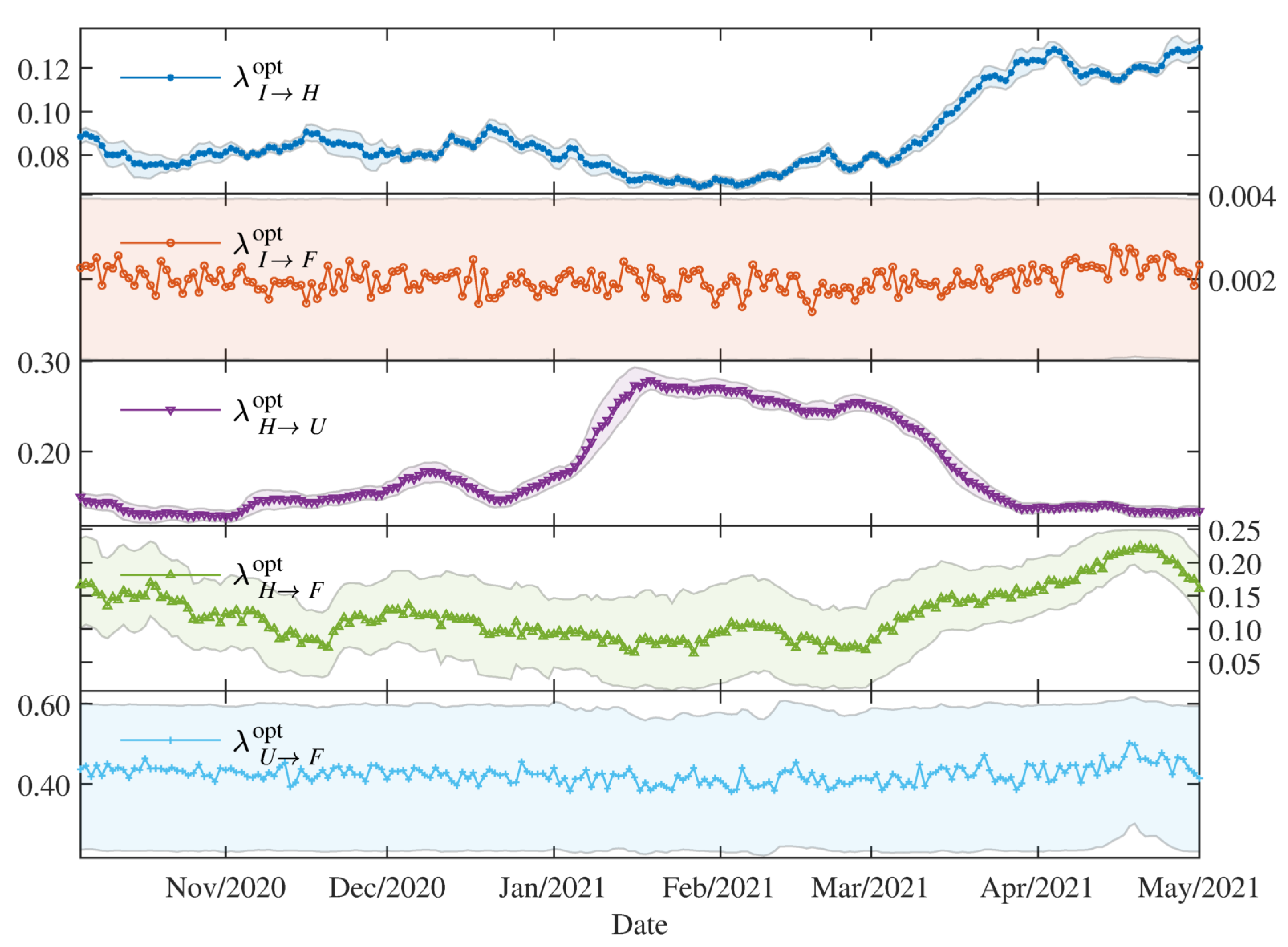
The estimated parameters helped us to interpret and analyse the spread dynamics of COVID-19 in different circumstances, which was particular in Paraguay. The relative error between the simulation results using the time-varying parameters and the available data is comparable to the relative deviation of the data using the moving time-window. This means that the simulation trajectories represent very well the variability in the population scale. The obtained transmissibility $\beta$ changes depending on the epidemic containment policies applied. And, the different proportions $\lambda$ are also changing due to the containment policies, but primarily on the availability of the beds and ICU in the hospitals. As the number of severe cases of COVID-19 patients becomes larger than the available beds and ICU in the hospitals, the proportions of deaths are also increasing.

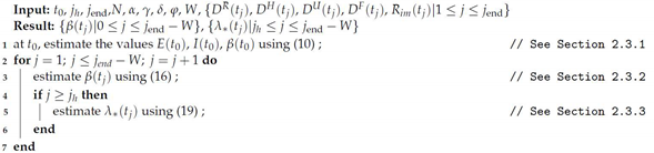
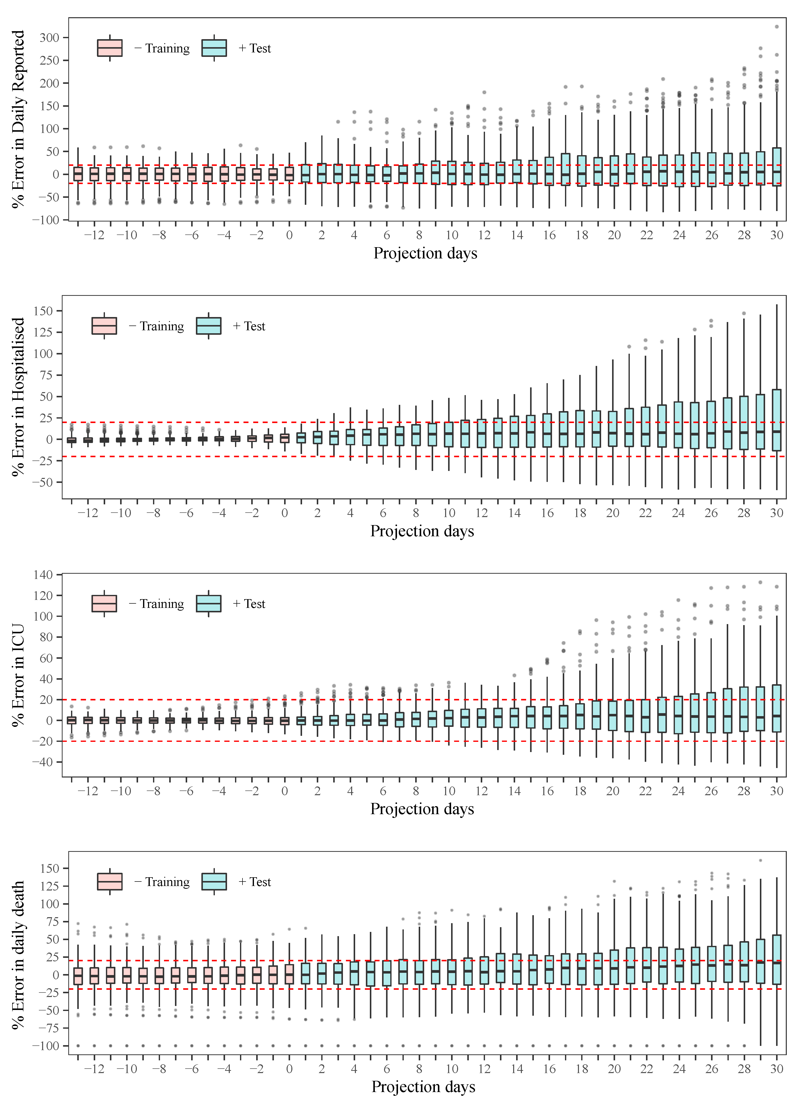
The statistical analysis of the behaviour of the error showed reasonable results [35], with a tendency to underestimate the observed data. This problem is somewhat inevitable considering the assumption of nearly constant parameters. As a decision-making tool, several scenarios can be drawn, for example: (i) plateau: by considering the transmissibility that stabilises daily reported infections as approximately a constant, (ii) the average value of transmissibility over the last month, (iii) 10% decrease in transmissibility when stronger quarantine measures are enforced, or (iv) 10% increase in transmissibility when quarantine measures are relaxed. All these scenarios can be based on the recently estimated parameters, which give additional advantages in the sense that, in one hand, the transmissibility of the disease can change over time due to the different strains of the viruses, and, on the other hand, after several containment measures, a portion of the population respecting the measures can vary compared to previous phases.

The early lockdown in Paraguay allowed for a slow increase in the number of COVID-19 patients, and thus, severe cases could be treated adequately by the health system until the beginning of 2021. Most of the time in 2020, the daily cases and deaths reported followed a plateau, but starting February 2021, cases increased substantially and the death proportions are becoming larger due to the collapse of the health system.

5. Relevance of the Work

Despite its simplicity, the SEIR-H model proposed in this work offers results relevant for the evolution of cases for COVID-19 in Paraguay. A visualisation tool for these results based on data from Paraguay is available at http://epymodel.uaa.edu.py (accessed on 12 October 2021). The Ministry of Public Health and Social Welfare and its Health Monitoring Centre in Paraguay use and reference this tool for analysis and decision-making (http://dgvs.mspbs.gov.py/page/#1387, accessed on 20 May 2021). Currently, results from this simple model are used to evaluate future scenarios and plan for resources allocation in the public health budget.

Results and projections obtained using the proposed SEIR-H model, exhibits similar statistical performance compared with other public platforms such as the COVID-19 Projections from IHME (Institute for Health Metrics and Evaluation) (https://covid19.healthdata.org/, accessed on 20 May 2021) [35] which serves as a reference for multiple governments and agencies. A sample comparison of the SEIR-H and IHME model results is presented in Appendix A.

6. Conclusions and Future Work

In this work, we proposed the SEIR-H epidemiological model with time-varying parameters in the form of step functions. This model is based on the classical SEIR model maintaining its simplicity in the spread dynamics of the disease. However, the SEIR-H model contains the dynamics of the occupations of normal beds and ICU in hospitals in order to guide decisions based on available hospital resources. This model was designed to have as few parameters as possible to be estimated, while still representing the dynamics observed in Paraguay.

We summarise the contributions of this work as follows:

• Integration of health system dynamics into the SEIR model, without losing the simplicity of the SEIR model.
• The methodology of parameter estimation for the time-varying parameters using a moving time-window, which allows us to determine the variability of the parameters according to the spread dynamics and social behaviour.
• The inclusion of the reported cases that were travellers from abroad in the inflow of reported cases, which is important at the beginning of an epidemic.
• Model assessment and statistical analysis of the error as a function of the projection horizon.
• Discussion of spread dynamics in Paraguay using the estimated parameters and trajectories obtained.

The proposed model has two main limitations. The first limitation is the assumption that all cases end up being reported ignoring the under-reporting of cases, which can be quite significant [36]. The second limitation is to ignore the limits of hospital capacity, both in terms of available care units for medium and severe cases. This issue is especially important for projections of deaths when the health system is overburdened [37]. Future work can address these aspects by adding a model for under-reported cases and by limiting the capacity of the health system.

Although, the SEIR-H model is fitted to the case of Paraguay, this model can be useful for any country or region to have a macroscopic overview of the dynamics of an epidemic like COVID-19, especially in contexts of limited availability of data detailing the heterogeneity of the population.

References

1. Doms, C.; Kramer, S.C.; Shaman, J. Assessing the Use of Influenza Forecasts and Epidemiological Modeling in Public Health Decision Making in the United States. Sci. Rep. 2018, 8, 12406. [Google Scholar] [CrossRef] [Green Version]
2. Anderson, R.M.; Heesterbeek, H.; Klinkenberg, D.; Hollingsworth, T.D. How will country-based mitigation measures influence the course of the COVID-19 epidemic? Lancet 2020, 395, 931–934. [Google Scholar] [CrossRef]
3. Sorci, G.; Faivre, B.; Morand, S. Explaining among-country variation in COVID-19 case fatality rate. Sci. Rep. 2020, 10, 1–11. [Google Scholar] [CrossRef]
4. Zimmer, C.; Corum, J.; Wee, S. Coronavirus Vaccine Tracker. Available online: https://www.nytimes.com/interactive/2020/science/coronavirus-vaccine-tracker.html (accessed on 20 May 2021).
5. Cooper, I.; Mondal, A.; Antonopoulos, C.G. A SIR model assumption for the spread of COVID-19 in different communities. Chaos Solitons Fractals 2020, 139, 110057. [Google Scholar] [CrossRef]
6. Ellison, G. Implications of Heterogeneous SIR Models for Analyses of COVID-19; Working Paper 27373; National Bureau of Economic Research: Cambridge, MA, USA, 2020. [Google Scholar] [CrossRef]
7. Crokidakis, N. Modeling the early evolution of the COVID-19 in Brazil: Results from a susceptible-infectious-quarantined-recovered (SIQR) model. Int. J. Mod. Phys. C 2020, 31, 2050135. [Google Scholar] [CrossRef]
8. He, S.; Peng, Y.; Sun, K. SEIR modeling of the COVID-19 and its dynamics. Nonlinear Dyn. 2020, 101, 1667–1680. [Google Scholar] [CrossRef]
9. Moghadas, S.M.; Fitzpatrick, M.C.; Sah, P.; Pandey, A.; Shoukat, A.; Singer, B.H.; Galvani, A.P. The implications of silent transmission for the control of COVID-19 outbreaks. Proc. Natl. Acad. Sci. USA 2020, 117, 17513–17515. [Google Scholar] [CrossRef] [PubMed]
10. Qian, G.; Yang, N.; Ma, A.H.Y.; Wang, L.; Li, G.; Chen, X.; Chen, X. COVID-19 transmission within a family cluster by presymptomatic carriers in China. Clin. Infect. Dis. 2020, 71, 861–862. [Google Scholar] [CrossRef] [PubMed]
11. Arino, J.; Portet, S. A simple model for COVID-19. Infect. Dis. Model. 2020, 5, 309–315. [Google Scholar] [CrossRef] [PubMed]
12. Giordano, G.; Blanchini, F.; Bruno, R.; Colaneri, P.; Di Filippo, A.; Di Matteo, A.; Colaneri, M. Modelling the COVID-19 epidemic and implementation of population-wide interventions in Italy. Nat. Med. 2020, 26, 855–860. [Google Scholar] [CrossRef]
13. Ramos, A.; Ferrández, M.; Vela-Pérez, M.; Kubik, A.; Ivorra, B. A simple but complex enough θ-SIR type model to be used with COVID-19 real data. Application to the case of Italy. Phys. D Nonlinear Phenom. 2021, 421, 132839. [Google Scholar] [CrossRef]
14. Arenas, A.; Cota, W.; Gómez-Gardeñes, J.; Gómez, S.; Granell, C.; Matamalas, J.T.; Soriano-Paños, D.; Steinegger, B. Modeling the Spatiotemporal Epidemic Spreading of COVID-19 and the Impact of Mobility and Social Distancing Interventions. Phys. Rev. X 2020, 10, 041055. [Google Scholar] [CrossRef]
15. Hethcote, H.W. Mathematics of infectious diseases. SIAM Rev. 2000, 42, 599–653. [Google Scholar] [CrossRef] [Green Version]
16. Feng, Z. Final and peak epidemic sizes for SEIR models with quarantine and isolation. Math. Biosci. Eng. 2007, 4, 675–686. [Google Scholar] [CrossRef]
17. Akaike, H. A New Look at the Statistical Model Identification. IEEE Trans. Autom. Control 1974, 19, 716–723. [Google Scholar] [CrossRef]
18. Peirlinck, M.; Linka, K.; Sahli Costabal, F.; Kuhl, E. Outbreak dynamics of COVID-19 in China and the United States. Biomech. Model. Mechanobiol. 2020, 19, 2179–2193. [Google Scholar] [CrossRef] [PubMed]
19. Roda, W.C.; Varughese, M.B.; Han, D.; Li, M.Y. Why is it difficult to accurately predict the COVID-19 epidemic? Infect. Dis. Model. 2020, 5, 271–281. [Google Scholar] [CrossRef] [PubMed]
20. Sjödin, H.; Wilder-Smith, A.; Osman, S.; Farooq, Z.; Rocklöv, J. Only strict quarantine measures can curb the coronavirus disease (COVID-19) outbreak in Italy, 2020. Eurosurveillance 2020, 25, 2000280. [Google Scholar] [CrossRef] [PubMed]
21. Wells, C.R.; Townsend, J.P.; Pandey, A.; Moghadas, S.M.; Krieger, G.; Singer, B.; McDonald, R.H.; Fitzpatrick, M.C.; Galvani, A.P. Optimal COVID-19 quarantine and testing strategies. Nat. Commun. 2021, 12, 356. [Google Scholar] [CrossRef]
22. Anderson, R.M.; May, R.M. Infectious Diseases of Humans: Dynamics and Control; Oxford University Press: Oxford, UK, 1992. [Google Scholar]
23. Furukawa, N.W.; Brooks, J.T.; Sobel, J. Evidence Supporting Transmission of Severe Acute Respiratory Syndrome Coronavirus 2 While Presymptomatic or Asymptomatic. Emerg. Infect. Dis. 2020, 26, e201595. [Google Scholar] [CrossRef] [PubMed]
24. He, X.; Lau, E.H.; Wu, P.; Deng, X.; Wang, J.; Hao, X.; Lau, Y.C.; Zhang, F.; Cowling, B.J.; Li, F.; et al. Temporal dynamics in viral shedding and transmissibility of COVID-19. Nat. Med. 2020, 26, 672–675. [Google Scholar] [CrossRef] [Green Version]
25. Wu, J.T.; Leung, K.; Leung, G.M. Nowcasting and forecasting the potential domestic and international spread of the 2019-nCoV outbreak originating in Wuhan, China: A modelling study. Lancet 2020, 395, 689–697. [Google Scholar] [CrossRef] [Green Version]
26. Peak, C.M.; Kahn, R.; Grad, Y.H.; Childs, L.M.; Li, R.; Lipsitch, M.; Buckee, C.O. Comparative Impact of Individual Quarantine vs. Active Monitoring of Contacts for the Mitigation of COVID-19: A modelling study. medRxiv 2020. [Google Scholar] [CrossRef]
27. Delamater, P.L.; Street, E.J.; Leslie, T.F.; Yang, Y.T.; Jacobsen, K.H. Complexity of the basic reproduction number (R0). Emerg. Infect. Dis. 2019, 25, 1–4. [Google Scholar] [CrossRef] [PubMed] [Green Version]
28. Smith, R.J.; Li, J.; Blakeley, D. The failure of R0. In Computational and Mathematical Methods in Medicine; Chu, H., Ed.; Hindawi Limited: London, UK, 2011; Volume 2011, p. 527610. [Google Scholar] [CrossRef] [Green Version]
29. Presidencia de la República del Paraguay. Decretos (COVID-19). Available online: https://www.mspbs.gov.py/decretos-covid19.html (accessed on 28 May 2021).
30. Presidencia de la República del Paraguay. Resoluciones (COVID-19). Available online: https://www.mspbs.gov.py/resoluciones-covid19.html (accessed on 28 May 2021).
31. Stan Development Team. RStan: The R interface to Stan. R Package Version 2.21.2 2020. Available online: http://mc-stan.org/ (accessed on 20 May 2021).
32. R Core Team. R: A Language and Environment for Statistical Computing. 2020. Available online: https://www.R-project.org/ (accessed on 20 May 2021).
33. Neal, R.M. MCMC using Hamiltonian dynamics. In Handbook of Markov Chain Monte Carlo; Jones, G., Meng, X.L., Gelman, A., Brooks, S., Eds.; Chapman and Hall/CRC: New York, NY, USA, 2011; Chapter 5; pp. 113–162. [Google Scholar] [CrossRef]
34. Li, Q.; Guan, X.; Wu, P.; Wang, X.; Zhou, L.; Tong, Y.; Ren, R.; Cowling, B.J.; Yang, B.; Leung, G.M.; et al. Early Transmission Dynamics in Wuhan, China, of Novel Coronavirus–Infected Pneumonia. N. Engl. J. Med. 2020, 382, 1199–1207. [Google Scholar] [CrossRef]
35. Friedman, J.; Liu, P.; Troeger, C.E.; Carter, A.; Reiner, R.C.; Barber, R.M.; Collins, J.; Lim, S.S.; Pigott, D.M.; Vos, T.; et al. Predictive performance of international COVID-19 mortality forecasting models. Nat. Commun. 2021, 12, 2609. [Google Scholar] [CrossRef]
36. Wu, S.L.; Mertens, A.N.; Crider, Y.S.; Nguyen, A.; Pokpongkiat, N.N.; Djajadi, S.; Seth, A.; Hsiang, M.S.; Colford, J.M.; Reingold, A.; et al. Substantial underestimation of SARS-CoV-2 infection in the United States. Nat. Commun. 2020, 11, 4507. [Google Scholar] [CrossRef]
37. Moghadas, S.M.; Shoukat, A.; Fitzpatrick, M.C.; Wells, C.R.; Sah, P.; Pandey, A.; Sachs, J.D.; Wang, Z.; Meyers, L.A.; Singer, B.H.; et al. Projecting hospital utilization during the COVID-19 outbreaks in the United States. Proc. Natl. Acad. Sci. USA 2020, 117, 9122–9126. [Google Scholar] [CrossRef] [Green Version]
Figure 1. Schematic diagrams of the SEIR-H model: the region in yellow indicates the transmission dynamics given by a SEIR with external reported cases, and the region in green represents the dynamics related to hospital resources. A more detailed version of the green region is used to show that the R compartment contains the dynamics related to the health system, represented mainly by H, U and F.
Applsci 11 09726 g001
Figure 2. The estimated transmissibility β opt with 95% credibility interval of the posterior distribution, obtained using the data of Paraguay. The horizontal line at 1 / 7 corresponds to the value of β that gives the basic reproduction number equivalent to one.
Applsci 11 09726 g002
Figure 3. Details of the data and simulations between May and June 2020. The results from the simulation are obtained using optimal β opt . Left vertical axis: the results of simulations and data; right vertical axis: transmissibility β opt .
Applsci 11 09726 g003
Figure 4. The proportions for the dynamics in the hospitals: the optimal values with the 95 credibility interval.
Applsci 11 09726 g004
Figure 5. The trajectories from the simulations using β opt ( t ) and λ * opt ( t ) compared to the data. Using the posterior distribution estimated on 1 April 2021, regions for trajectories are shown for one month ahead with percentile 95 credibility intervals.
Applsci 11 09726 g005
Figure 6. Statistical behaviour of the error as a function of the projection horizon.
Applsci 11 09726 g006