Optimal Reserve and Energy Scheduling for a Virtual Power Plant Considering Reserve Activation Probability

Abstract

With the increasing share of variable and limitedly predictable renewable energy in power systems worldwide, ensuring reserve capacity to maintain the balance of supply and demand becomes more important. On the other hand, the development of the virtual power plant model (VPP) allows renewable sources and energy storage to participate in reserve service. This paper addresses the optimal reserve bidding strategy problem of a VPP comprising of renewable energy resources (RESs), energy storage systems (ESSs), and several customers. The VPP participates in balance capacity (BC), day-ahead (DA), and intra-day (ID) markets. The scheduling problem is formulated as a two-stage chance-constrained optimization model taking the uncertainty of RESs production, load consumption, and probability of reserve activation into account. The response of VPP after its reserve capacity is called and generated is also considered to increase the operational flexibility of VPP. The proposed model is implemented on a test VPP system, and the effects of RESs sizing, ESSs sizing, and the probability of reserve activation are analyzed. Results indicate that the proposed model can perform well under real-world conditions.

1. Introduction

In recent years, due to the ever-increasing electricity demand and environmental problems, renewable energy sources (RESs), such as wind and solar power, have been quickly developed and have become an essential part of the electricity system. Many governments have provided incentives to increase investments in renewable energy plants, for example, allowing these sources to participate in the electricity market or provide regulation reserve service [1,2]. However, integrating RESs into the electricity market faces several challenges. The authors of [3,4,5,6] show that most electricity markets, such as PJM and AESO, require the participating resources to be at least 100 kW of capacity. Meanwhile, the rated capacity of RESs is typically small, especially rooftop solar systems in which sizing can be less than 10 kW. Another disadvantage of RESs is the stochastic nature of wind speed and solar radiation, meaning RESs maximum available power output can not be predicted with high accuracy. As a result, it is difficult to ensure that RESs can meet the registered schedule in the electricity market.

To overcome these issues, the concept of the virtual power plant (VPP) has been developed. A VPP aggregates the capacity of different types of RESs, flexible loads, energy storage systems (ESS), and acts as a single participant in the wholesale market [7,8,9,10]. A VPP can play two roles in the market: a supplier or a consumer, depending on the sizing of RESs and ESS in comparison to local demand. This paradigm shift allows small-scale resources to participate in the market and makes them more profitable [9,11]. This is because the operation of RESs, controllable demand, and ESS are coordinated; consequently, the available power output of each RES can be fully utilized while the surplus or lack of power due to predictive errors can also be compensated. By using advanced information and communication technology and control systems, a VPP can even manage and control many resources that may be dispersed in different points in a grid [11]. Research by Pudjianto et al. [11] shows that a VPP can be classified into two operational levels, depending on the economic or technical viewpoint: the Commercial VPP (CVPP) and the Technical VPP (TVPP). The CVPP bids in the wholesale market, which decides each RES scheduling to maximize profits. It can be seen that the CVPP only focuses on economic issues and does not consider the network constraints. Meanwhile, the TVPP’s task is to receive the operating parameters of all resources from the CVPP, perform system management, and provide transmission balancing services. The TVPP should take the network diagram and transmission congestions into account in its operational planning.

With the integration of a large amount of RES, ESS, and loads, a VPP has the ability to participate in many different power markets such as the day-ahead (DA) market, intraday (ID) market, balancing capacity (BC) market, or balancing energy (BE) market. Naval and Yusta [12] show that many studies focus on developing a VPP’s operating model to achieve optimal coordination between components in the VPP, thereby maximizing VPP profits. References [13,14,15] focus on the optimal schedule of a VPP in a two-settlement electricity market, including DA and ID markets. Meanwhile, studies [8,16,17] consider the role of a VPP in the reserve market. In these papers, the day-ahead market is cleared at noon, and a VPP should propose its bid for each hour of the following day before the end of the trading period. The prediction errors of demand and RESs power output will cause power imbalances in the real-time operation. A VPP can access the BE market as a regulator when the balancing price is cleared at least one hour before operation time. Another study [18] proposes a new market bid format that allows a VPP to act as either an active or passive regulator in the BE market. The result shows that this market model allows a VPP to gain higher profits. Meanwhile, study [19] considers the demand response exchange (DRX) market, which allows a VPP to buy demand response services (DR) to reduce the imbalance cost in the BE market.

A few other works focus on the VPP’s reserve trading in the BC market, which plays an essential role in maintaining the system frequency and stability. Mashhour and Moghaddas-Tafreshi [8] investigate the bidding strategy of a VPP in the joint energy and spinning reserve market. The authors consider only the reserve energy market while the adequacy reserve maintained by a VPP is a predetermined parameter. Several more recent studies [20,21,22] propose multi-stage scheduling models considering the BC market. In these papers, the VPP trades the reserve capacity simultaneously as energy trading in the day-ahead market. By contrast, the reserve capacity contract in practice should be determined several days before the day-ahead market, depending on the electricity market’s rules in each country and the balancing product [23,24,25]. It is easy to see that computing the optimal reserve capacity trading is problematic because it is impossible to accurately predict the RES available power output and the local load.

On the other hand, a reserve contract not only requires scheduling RESs less than the forecasting available power but also forces the ESS to maintain a minimum energy level to provide reserve service, thereby reducing the role of ESS in supplying the load. It can be seen that the probability of a power shortage depends on the penetration level of RES or demand. If the probability of reserve activation is quite small, the VPP’s profit in the BC market may not be higher than the reduction in its profit in the day-ahead market. However, a few works consider the probability of reserve activation when determining the optimal reserve contract, such as [26,27]. Moreover, these studies are implemented from the perspective of the grid manager, whose task is to optimally distribute the reserve capacity to all plants in the main grid, rather than to optimize individual power plants’ profit.

This paper proposes a two-stage scheduling problem of a CVPP, including RES units, ESSs, and demand. The CVPP participates in both reserve capacity and energy markets. The primary goal is to determine the VPP’s optimal reserve contract to maximize the VPP’s profit while still considering its operating scheme in the energy market. The optimal scheduling problem is formulated as a two-stage chance-constrained optimization model to account for the uncertainty in RESs available power output and demand. The constraints, including uncertain parameters, are presented as probabilistic constraints with a chosen risk level [28]. This chance-constrained model can be solved by the Sample Average Approximation (SAA) algorithm, which is based on a Monte Carlo simulation to approximate each random parameter by a vector of N samples. The studies [29,30,31,32] show the effectiveness of this approach. Moreover, the probability of reserve activation is taken into account in this paper to ensure that the VPP can provide reserve service during the hours having the greatest risk of power shortages.

The salient features of the present study include the following:

• The research focuses on the VPP’s optimal reserve sizing problem considering the probability of reserve activation each hour. Depending on the status of reserve activation, the VPP’s operating scheme in electricity markets is determined to maximize the VPP’s profit.
• The proposed optimal model is based on a two-stage chance-constrained problem which allows a certain risk level in the VPP’s scheduling. This model is suitable for the short-term planning of power systems with uncertain resources and demand.
• The impact of ESS sizing, RES sizing, and the probability of reserve activation on the VPP’s optimal reserve sizing is analyzed.

The rest of the paper is organized as follows: Section 2 demonstrates the operating model of the VPP in the BC and electricity markets as well as the assumptions used in this paper, thereby presenting a two-stage optimization model to determine the VPP’s optimal reserve capacity. Section 3 presents the mathematical formulation of the proposed optimization model. Then, the computation results are collected and analyzed in Section 4. Finally, Section 5 concludes the paper.

2. Problem Description

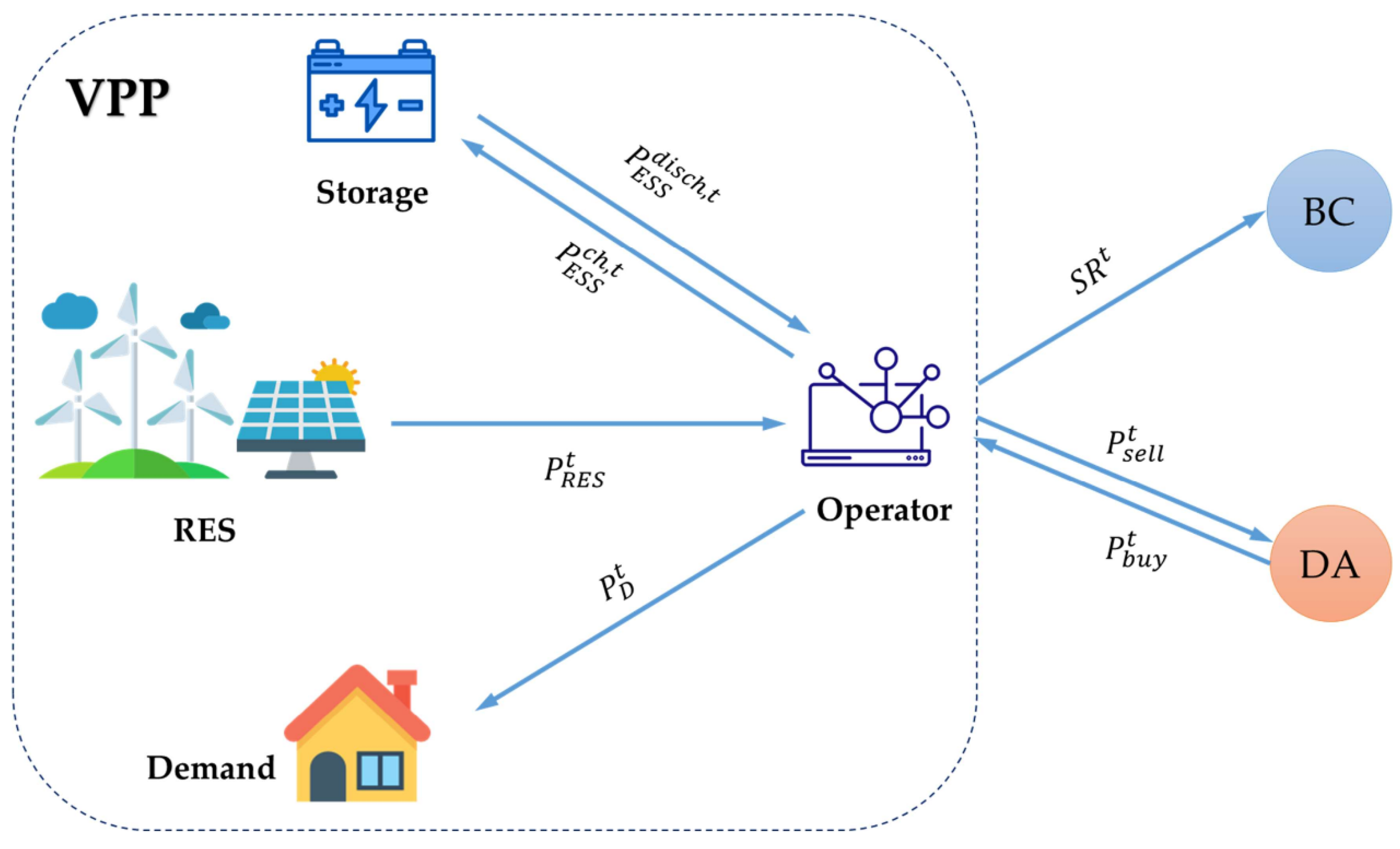
2.1. Coordination between the VPP and the Power Market

With the high penetration of RESs in the power system, the grid’s operational framework changes. References [33,34] show that installing and connecting the ESS in the power system to support RESs provides ancillary services, and leverage energy arbitrage opportunities are increasingly interested. Some electricity markets, such as AEMO, have changed their rules to allow privately owned ESSs and RESs to participate in the electricity market. Accordingly, the VPP model is getting more and more attention.

This paper considers a CVPP consisting of RESs, ESSs, and demand, as shown in Figure 1. The VPP can participate in the DA market, both as supplier and consumer, i.e., the VPP either sells or purchases electricity from the main grid, depending on whether RESs available power output is higher or less than the local demand. The ESS also allows VPPs to trade in the BC market. While the ESS has a high investment cost, it has very low operating costs and the ability to change power output very quickly. Therefore, ESS can serve as an efficient reserve source compared to other alternatives, such as demand response or RES curtailment [34].

The BC market, in which supplier and demand trade their reserve capacity, plays an essential role in worldwide power systems. It can be seen that the transmission system operators (TSOs) should match the supply and demand to maintain frequency and achieve system stability. However, events such as prediction errors and power outages are unpredictable, and TSOs, therefore, need to be able to adjust for such unexpected power fluctuations. On the other hand, the power generation company shuts down unnecessary generators when there is no buyer, and restarting these units requires at least a few hours. The BC market helps the TSOs secure the number of generators (or the amount of capacity) that can be adjusted in advance.

The BC market has regulations on contract duration, minimum bid amount, and continuous operation time corresponding to each BC product in all countries. For example, the Japan electricity market requires that the BC market should be cleared before the operating day, at least one day for tertiary reserve-2, and at least one week for the other four types of reserve (

Table 1. Japanese BC market’s requirement [25].

	Primary Control Reserve	Secondary Control Reserve 1	Secondary Control Reserve 2	Tertiary Control Reserve 1	Tertiary Control Reserve 2
	GF Control Equivalent	LFC	EDC	EDC
Response time	Within 10 s	Within 5 min	Within 5 min	Within 15 min	Within 15 min
Continuous operation time	At least 5 min	At least 5 min	At least 30 min	3 h	3 h
Clearing time	1 week ago	1 week ago	1 week ago	1 week ago	1 day ago
Minimum bid amount	5 MW	5 MW	5 MW	5 MW	5 MW

). Moreover, each generation plant with a BC contract must supply a reserve capacity of at least 5 MW and maintain it for the required duration. Although the classification of reserve services may vary from country to country, they generally have similar requirements [24,35], and a VPP should satisfy these requirements to participate in the BC market.

If a VPP joins the BC market, the VPP operator must solve the problem of determining its BC trading to maximize the total profit in both BC and DA markets. It should be noted that the profit obtained from the BC market consists of two parts: profit from the provision of reserve capacity and profit from the activation of reserve service. The VPP operator does not know whether its reserve service will be called and how much electric power will be generated for the reserve. It can be seen that if the VPP is not called to provide reserve service, its total profit may be lower than in the case that its full available capacity is sold to the energy market. Thus, the probability of reserve activation should be considered in the profit maximization problem from the BC market.

It is assumed that the VPP has a contract to provide reserve capacity, as described in Figure 2. In each hour of this period, the VPP is faced with two possibilities of either being called or not being called to provide reserve service. Considering ESSs integrated into the VPP, it can be seen that whether reserve capacity is fully/partly activated or not will affect the energy stored in the VPP. In addition, unlike the conventional power plants that commonly maintain a certain ramp magnitude, the maximum available power output of RESs is expected to be utilized without any curtailment. It can be solved by adjusting the day-ahead operating schedule in the intraday market (Figure 2). However, this adjustment must ensure that the VPP has enough energy to provide reserve service during the next contracting period.

From the VPP operator’s point of view, a two-stage scheduling model is proposed to maximize the VPP’s profit in the reserve capacity and energy markets. This model determines the optimal reserve capacity and the possible operating scenarios of the VPP in the day-ahead and intraday markets. The uncertainty in RES and demand and the probability of reserve activation will be considered in this model.

The two stages are outlined as follows:

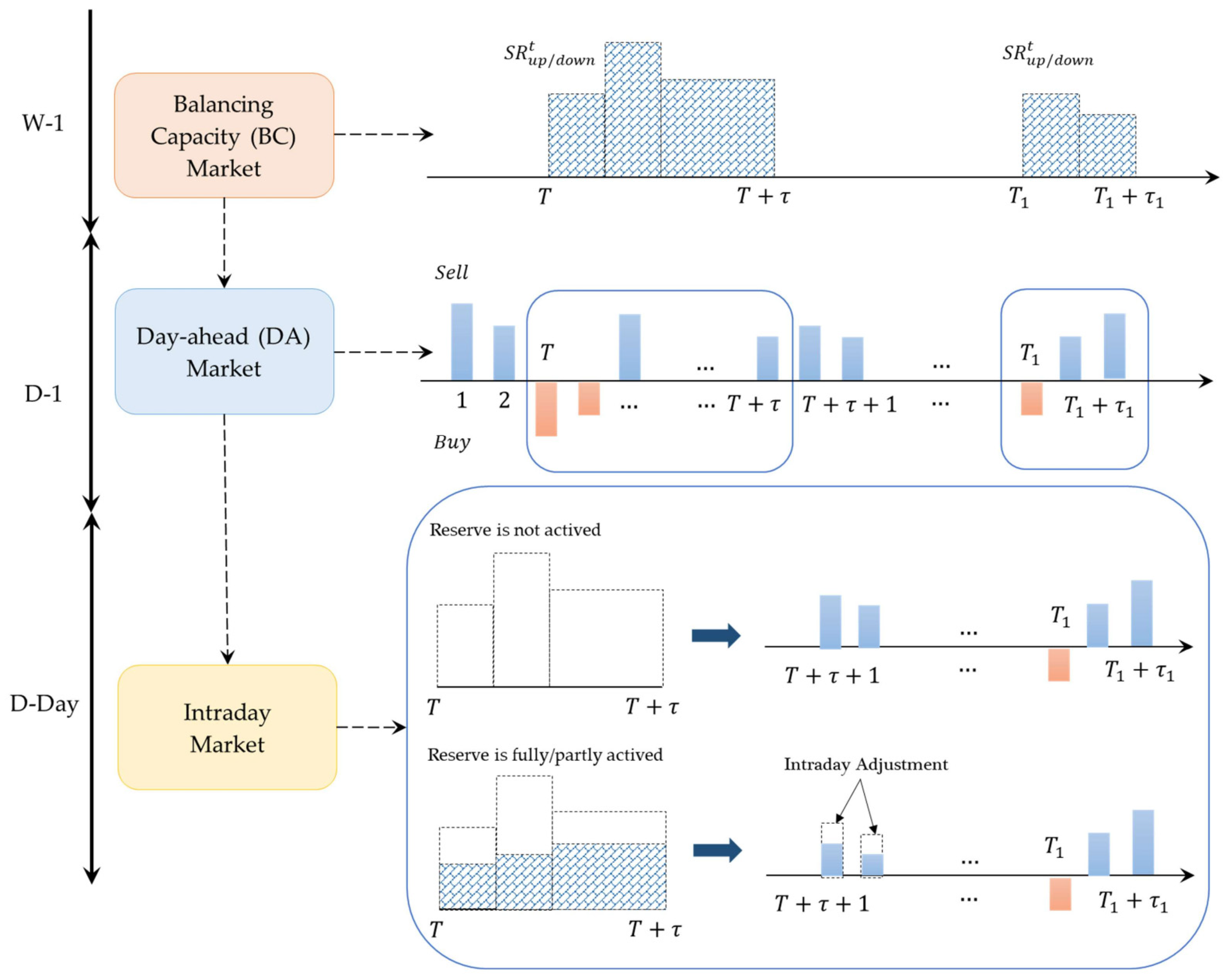
• In the first stage, the VPP decides its trading strategy in the BC market a few days before operating based on the long-term forecasted value. The reserve capacity $S{R}^t$should be higher than the minimum bid amount and be maintained over the required continuous operating duration ${\tau }_{iON}$. The variable $S{R}^t$is a here-and-now decision made before the realization of uncertain parameters.
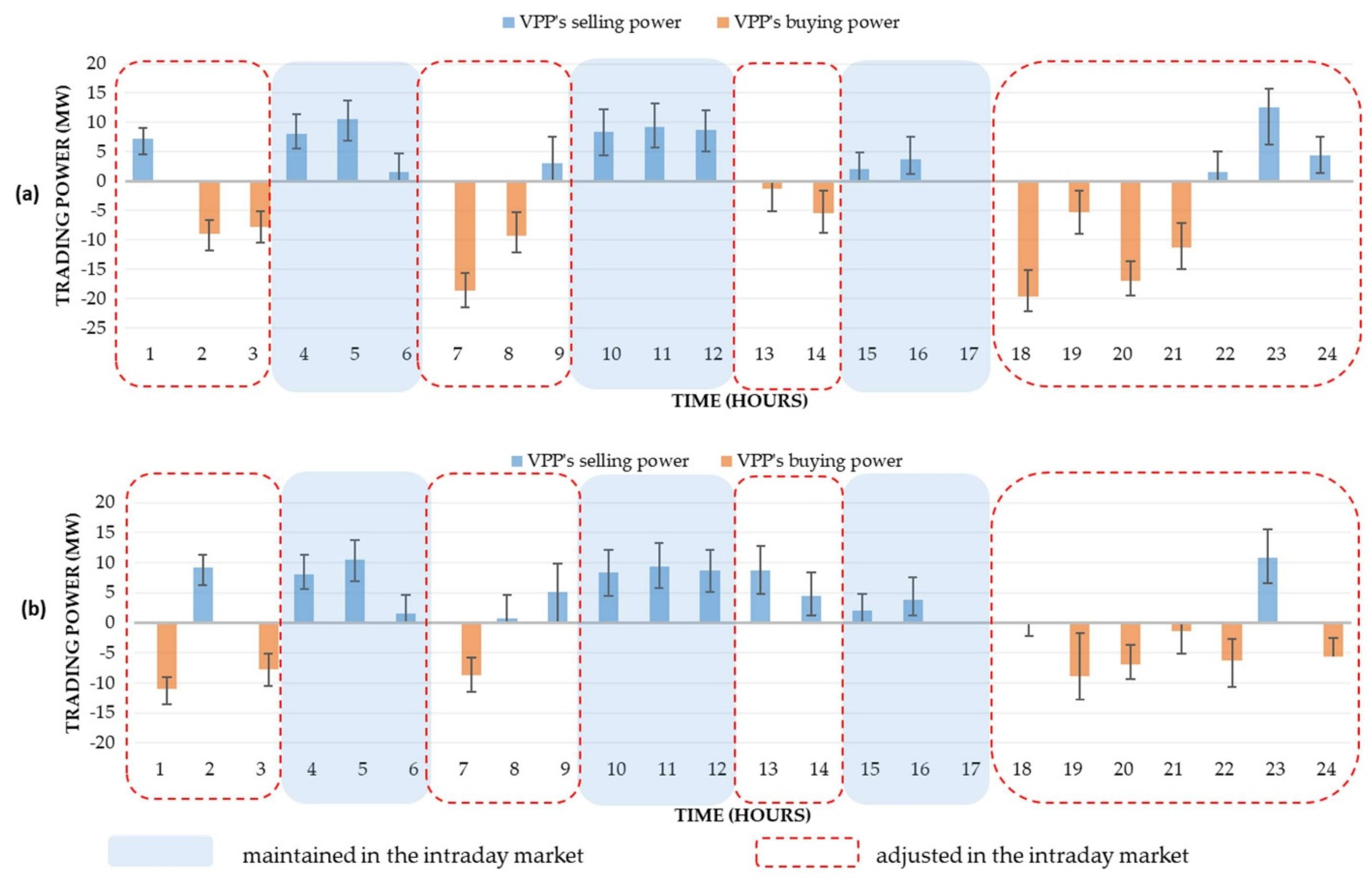
• After determining $S{R}^t$, the VPP should predict its energy trading scenarios $P_{sell}^t/P_{buy}^t$ at hour t on the operating day. These scenarios are based on long-term forecasts and will be revised in the day-ahead market with the short-term forecast figures for load and RESs. At the same time, the scenarios of reserve activation are also taken into account to predict the amount of buying/selling energy that needs to be adjusted in the intraday market.

To simplify the model, we consider only two extreme scenarios of reserve activation: the entire reserve/no reserve is activated, where the probabilities of these cases in hour t are assumed to be $p_{SR}^t$, and $\left(1-p_{SR}^t\right)$, respectively.

2.2. Uncertainty Parameters

A major challenge in implementing the two-stage model in the previous section is the variation in demand and RESs power output. It can be seen that this scheduling model is solved several days in advance; at that time, information on demand and RESs power output is uncertain and unknown. Therefore, uncertainties of demand and RESs power output should be taken into account in this model to ensure that the results are meaningful in the actual operation.

A common method to handle these uncertain parameters is to represent them as the sum of the predicted value and predictive errors as follows:

$$\{\begin{array}{c}{P}_{RESmax}^t=P_{RESf}^t+P_{RES-error}^t{P}_{RESf}^t\\ P_D^t=P_{Df}^t+P_{D-error}^t{P}_{Df}^t\end{array}$$

(1)

where the errors $P_{RES-error}^t$ and $P_{D-error}^t$ have a normal distribution function with means of 0, and the standard deviations ${\sigma }_{RES}^t$ and ${\sigma }_D^t$, respectively. This means that the maximum difference between the actual value and the forecasted data would be approximately $3{\sigma }_{RES}^t$ for RESs available power and $3{\sigma }_D^t$ for demand.

Another important uncertain parameter is the probability that the reserve is called and generated in each hour. Determining this parameter is difficult because it depends on many factors such as generator outages, line outages, market price, or bidding strategy. While Y. Yamin [36] focuses on predicting the reserve probability based on an artificial neural network (ANN), other studies [26,37,38] use the loss of load probability (LOLP) or the expected energy not served (EENS) to determine the reserve requirements and build the reliability-constrained unit commitment model. A recent study [39] builds the probability functions of the reserve activation based on historical observations for the period 2015–2018, obtained from Elia, the Belgian transmission system operator. Then, this probability function is applied to determine the ESS scheduling in the day-ahead energy and reserve market.

In this paper, the reserve activation probability in each hour is assumed to be an independent random variable that follows the uniform distribution function and can be predicted from historical outage data:

$$p^t~U\left(0,p^{max}\right)$$

(2)

where $p^{max}$ is the maximum possible value of the reserve activation probabilities obtained from historical data.

3. Mathematical Formulation

This article deals with the optimal scheduling strategy of a VPP, including RES units, ESS, and demand, which aims to participate in both the BC and the energy markets. Based on the forecasted data of demand and RES available power output, the VPP operator calculates its reserve capacity and the amount of energy that can be sold or purchased each hour. Consequently, the RESs operating schedules and the ESS charge/discharge states are determined to maximize the total revenue of the VPP obtained in both the BC and the energy markets.

The VPP decisions under uncertainty are handled by two-stage chance-constrained programming. In the first stage, VPP reserve capacity $S{R}^t$ is decided for every hour during a 24-h horizon. Other operational parameters of the VPP, such as the energy trading with the main grid or the ESS charge/discharge power, are determined in the second stage. As can be seen, the first-stage decision has only one value held until the actual operation time. By contrast, the second-stage decisions are expressed as a range of values to ensure the availability of these decisions if the actual data differ from the predicted value. In addition, the second-stage decisions can be adjusted as soon as the latest short-term forecast data with high accuracy are available. Using the chance-constrained model ensures that the constraints in this problem are met with a chosen probability even if the predictive errors are quite high.

3.1. Objective Function

The objective function of the proposed problem is to maximize the VPP profit including profit from both the BC market and the energy market. With two scenarios and corresponding probabilities presented in the previous section, the objective function can be formulated as follows:

$$Maximize F={\displaystyle \sum }_{t=1}^{24}S{R}^t c_{SRbase}+p_{SR}^{t}S{R}^t c_{SR}^t+\mathbb{E}\left[\begin{array}{c}{p}_{SR}^t\left(P_{sell,1}^t\left(\xi \right)c_{sell}^t-P_{buy,1}^t\left(\xi \right)c_{buy}^t\right)+\\ \left(1-p_{SR}^t\right)\left(P_{sell,2}^t\left(\xi \right)c_{sell}^t-P_{buy,2}^t\left(\xi \right)c_{buy}^t\right)\end{array}\right]$$

(3)

In the above equations, $\xi$ represents a random vector including RESs available power and demand.

3.2. Constraints

The proposed problem is formulated based on two cases of reserve activation. Therefore, the market participation model and the operation of each component in the VPP are accomplished under the first-stage constraints and two sets of the second-stage constraints as follows:

3.2.1. The First-Stage Constraints:

In this model, the first-stage constraints describe the reserve capacity trading between the VPP and BC market. Equation (4) ensures that the reserve capacity should be limited by the rated power of the RES and ESS. With the binary variable $u_{SR}^t$ equal to 1 if the VPP decides to sell reserve capacity, Equation (4) ensures that the VPP can maintain reserve service for a period of at least ${\tau }_{iON}$. Then, this service can stop for a period of ${\tau }_{iOFF}$before a new regulation period, ${\tau }_{iOFF}$ can be set to zero.

$$\{\begin{array}{c}0\le S{R}^t=P_{RES-SR}^t+P_{ESS-SR}^t\le u_{SR}^t\left(P_{ESSmax}+P_{RESrated}\right)\\ u_{SR}^t-u_{SR}^{t-1}=u^t-v^t\\ {\displaystyle \sum _{k=t-{\tau }_{iON}}^t}{u}^k\le u_{SR}^t\\ {\displaystyle \sum _{k=t-{\tau }_{iOFF}}^t}{v}^k\le 1-u_{SR}^t\end{array}$$

(4)

3.2.2. The Second-Stage Constraints

• Case 1: The reserve bid is activated:

• RES operating constraint: For a given forecasted available power $P_{RESf}^t$ and the minimum power threshold $P_{RESmin}^t$, the power output of the RES must satisfy Equation (5). Equation (6) shows that RES can supply electricity directly to the local loads and contribute to the contract of the VPP in the BC market and the DA market. Besides, RES’s excess energy (if any) is stored in the ESS to utilize RES’s available power output.

  $$u_{RES}^t\left(\xi \right)P_{RESmin}^t\le P_{RES,1}^t\left(\xi \right)\le u_{RES}^t\left(\xi \right)\left(P_{RESf}^t+P_{RES-error}^t{P}_{RESf}^t\right)$$

  (5)

  $$P_{RES,1}^t\left(\xi \right)=P_{RES-SR}^t+P_{RES-grid,1}^t\left(\xi \right)+P_{RES-load,1}^t\left(\xi \right)+P_{RES-ESS,1}^t\left(\xi \right)$$

  (6)
• ESS constraints: This article uses ESS to store the excess power of RESs or purchased power from the DA market if the electricity price is low. The stored energy will be released to supply the peak load of VPP or sell to both BC and DA markets if the electricity price is high. Equations (7) and (8) show that the charging/discharging power of the ESS is limited by the rated power $P_{ESSmax}$. In these constraints, the binary variable $u_{SS}^t$ makes sure that the ESS can only be in one state: charging or discharging. Equation (9) shows that the energy $E_{SS}^t$ stored in the ESS should be limited by its rated capacity at all times. Furthermore, Equation (10) makes sure that the energy stored in the ESS will be set to a certain value after each operating day.

  $$0\le P_{ESS,1}^{ch,t}\left(\xi \right)=P_{RES-ESS,1}^t\left(\xi \right)+P_{grid-ESS,1}^t\left(\xi \right)\le u_{SS,1}^t\left(\xi \right)P_{ESSmax}$$

  (7)

  $$0\le P_{ESS,1}^{disch,t}\left(\xi \right)=P_{ESS-SR}^t+P_{ESS-grid,1}^t\left(\xi \right)+P_{ESS-load,1}^t\left(\xi \right)\le \left(1-u_{SS,1}^t\left(\xi \right)\right)P_{ESSmax}$$

  (8)

  $$E_{ESSmin}\le E_{ESS,1}^t\left(\xi \right)=E_{ESS,1}^{t-1}\left(\xi \right)+\eta P_{ESS,1}^{ch,t}\left(\xi \right)-P_{ESS,1}^{disch,t}\left(\xi \right)/\eta \le E_{ESSmax}$$

  (9)

  $$E_{ESS}^{t=0}=E_{ESS}^{t=24}$$

  (10)
• Day-ahead market’s constraints: Constraints (11) and (12) show the role of RES and ESS in the DA market. Meanwhile, constraint (13) shows that the arbitrage between the BC and the DA market is not permitted. This means that the VPP is not allowed to buy electricity from the DA in order to sell to the BC market at the same time.

  $$0\le P_{sell,1}^t\left(\xi \right)=P_{RES-grid,1}^t\left(\xi \right)+P_{ESS-grid,1}^t\left(\xi \right)\le \left(1-u_{buy,1}^t\right)\left(P_{ESSmax}+P_{RESrated}\right)$$

  (11)

  $$0\le P_{buy,1}^t\left(\xi \right)=P_{grid-load,1}^t\left(\xi \right)+P_{grid-ESS,1}^t\left(\xi \right)\le u_{buy,1}^t\left(P_{ESSmax}+Loa{d}_{max}\right)$$

  (12)

  $$u_{buy}^t+u_{SR}^t\le 1;$$

  (13)
• Active power balance constraint: The VPP’s operator must balance demand and supply in all operating scenarios. If the reserve bids are called on to produce, the total active power output from RES and ESS must meet the demand and the power supplied to the main grid according to the signed BC and DA contract. This equation is formulated as a probability constraint to guarantee that the probability of power imbalance is less than a risk level $\epsilon$, even if the difference between the real-time data and the predicted value of $\xi$ is quite high.

  $$\mathrm{Pr}\left(P_{RES,1}^t\left(\xi \right)+P_{ESS,1}^{disch,t}\left(\xi \right)+P_{buy,1}^t\left(\xi \right)=S{R}^t+P_{sell,1}^t\left(\xi \right)+P_{ESS,1}^{ch,t}\left(\xi \right)+P_{Df}^t+P_{D-error}^t{P}_{Df}^t\right)\ge 1-\epsilon$$

  (14)

2.

Case 2: The reserve bid is not activated:

Similar to case 1, the constraints in case 2 are shown as follows:

• RES operating constraint:

  $$u_{RES}^t\left(\xi \right)P_{RESmin}^t\le P_{RES,2}^t\left(\xi \right)+P_{RES-SR}^t\le u_{RES}^t\left(\xi \right)\left(P_{RESf}^t+P_{RES-error}^t{P}_{RESf}^t\right)$$

  (15)

  $$P_{RES,2}^t\left(\xi \right)=P_{RES-grid,2}^t\left(\xi \right)+P_{RES-load,2}^t\left(\xi \right)+P_{RES-ESS,2}^t\left(\xi \right)$$

  (16)
• ESS constraints:

  $$0\le P_{ESS,2}^{ch,t}\left(\xi \right)=P_{RES-ESS,2}^t\left(\xi \right)+P_{grid-ESS,2}^t\left(\xi \right)\le u_{SS,2}^t\left(\xi \right)P_{ESSmax}$$

  (17)

  $$\{\begin{array}{c}0\le P_{ESS,2}^{disch,t}\left(\xi \right)=P_{ESS-grid,2}^t\left(\xi \right)+P_{ESS-load,2}^t\left(\xi \right)\le \left(1-u_{SS,2}^t\left(\xi \right)\right)P_{ESSmax}\\ P_{ESS,2}^{disch,t}\left(\xi \right)+P_{ESS-SR}^t\le P_{ESSmax}\end{array}$$

  (18)

  $$E_{ESSmin}\le E_{ESS,2}^t\left(\xi \right)=E_{ESS,2}^{t-1}\left(\xi \right)+\eta P_{ESS,2}^{ch,t}\left(\xi \right)-P_{ESS,2}^{disch,t}\left(\xi \right)/\eta \le E_{ESSmax}$$

  (19)
• Day-ahead market’s constraints:

  $$0\le P_{sell,2}^t\left(\xi \right)=P_{RES-grid,2}^t\left(\xi \right)+P_{ESS-grid,2}^t\left(\xi \right)\le \left(1-u_{buy}^t\right)\left(P_{ESSmax}+P_{RESrated}\right)$$

  (20)

  $$0\le P_{buy,2}^t\left(\xi \right)=P_{grid-load,2}^t\left(\xi \right)+P_{grid-ESS,2}^t\left(\xi \right)\le u_{buy}^t\left(P_{ESSmax}+Loa{d}_{max}\right)$$

  (21)
• Active power balance constraint:

  $$\mathrm{Pr}\left(P_{RES,2}^t\left(\xi \right)+P_{ESS,2}^{disch,t}\left(\xi \right)+P_{buy,2}^t\left(\xi \right)=P_{sell,2}^t\left(\xi \right)+P_{ESS,2}^{ch,t}\left(\xi \right)+P_{Df}^t+P_{D-error}^t{P}_{Df}^t\right)\ge 1-\epsilon$$

  (22)

3.

Constraint shows the association between case 1 and case 2:

During the reserve contract period, it is necessary to ensure that the VPP is always ready to provide reserve at any time. Therefore, even if the reserve is not called and generated, the VPP is not allowed to sell that part of the capacity to the energy market. Consequently, the VPP’s buying/selling power in the energy market should be the same for cases 1 and 2. When there is no reserve contract, the VPP’s buying/selling power is allowed to be adjusted to take full advantage of the power output of the RESs. In addition, since the ESS provides a part of reserve capacity, the energy in the ESS immediately before the contract period should be the same in both cases. The following constraints can secure these issues:

$$\{\begin{array}{c}-\left(1-u_{SR}^t\right)bigM\le P_{sell,1}^t\left(\xi \right)-P_{sell,2}^t\left(\xi \right)\le \left(1-u_{SR}^t\right)bigM\\ -\left(1-u_{SR}^t\right)bigM\le P_{buy,1}^t\left(\xi \right)-P_{buy,2}^t\left(\xi \right)\le \left(1-u_{SR}^t\right)bigM\end{array}$$

(23)

$$-\left(1-u_{SR}^t+u_{SR}^{t-1}\right)bigM\le E_{ESS,1}^{t-1}\left(\xi \right)-E_{ESS,2}^{t-1}\left(\xi \right)\le \left(1-u_{SR}^t+u_{SR}^{t-1}\right)bigM$$

(24)

3.3. Sample Average Approximation Methodology

The two-stage chance-constrained optimization model in the above section can be solved by the sample average approximation approach. In this approach, the true distribution of each uncertain parameter is approximated by a set of independent samples by using a Monte Carlo simulation while the corresponding sample average function replaces the objective function. Many studies in the literature show that SAA effectively solves a chance-constrained optimization problem [28,29,34,35,36,37]. However, it can be seen that the more uncertain parameters, the larger the size of the optimization problem and the longer the computing time. To overcome this challenge, a common technique to improve computational efficiency is using clustering methods such as K-means, Fuzzy C-means methods [38,39]. This technique reduces a large number of initial samples into a small number of clusters, then these clusters are represented as a new set of samples and used to solve the SAA problem.

Algorithm 1 outlines the main steps of the SAA algorithm combined K-means approach to solve a general chance-constrained optimization problem as follows:

$$V=\min \left\{f\left(x\right)+\mathbb{E}\left(Q\left(y,\xi \right)\right)\right\}$$

(25)

subject to

$$\mathrm{Pr}\left(G\left(x,y,\xi \right)\le 0\right)\ge 1-\epsilon$$

(26)

where $x$ is the first-stage variable, $y$ is the second-stage variable, $\xi$ is random input data, and $\epsilon$ is the risk level of the chance constraint in the problem (25).

In the first step, we generate M independent sample sets of size N. Then, the k-means clustering approach is applied to divide each set into N_L clusters. Each cluster’s centroid will be considered a scenario in SAA algorithm with its probability is equal to the total probabilities of all samples inside the cluster. Consequently, the optimization problem in Equations (25) and (26) are reformulated as:

$$V=\min \left\{f\left(x\right)+{\displaystyle \sum }_{n=1}^{N_L}{p}_{n}Q\left(y_n,{\xi }_n\right)\right\}$$

(27)

subject to

$${\displaystyle \sum }_{n=1}^{N_L}{p}_n{\mathbf{1}}_{\left(0,\infty \right)}\left(G\left(x,y_n,{\xi }_n\right)\right)\le \gamma$$

(28)

where ${\mathbf{1}}_{\left(0,\infty \right)}\left(G\left(x,y_n,{\xi }_n\right)\right)$ is equal to one if $G\left(x,y_n,{\xi }_n\right)\ge 0$ and zero otherwise, $p_n$ is nth centroid’s probability ($n=1,2,\dots ,N_L)$, and $\gamma$ is the risk level of the SAA model (27) $\left(0\le \gamma \le \epsilon \right)$.

Based on the method presented in [29,40], the SAA problem (27) is implemented S iterations. In each iteration, this model will be solved M times in correspondence to M sample sets so that we can obtain M first-stage optimal solutions $x_s^m$ and optimal values $V_s^m$ ($1\le s\le S, 1\le m\le M).$As the optimal problem contains chance constraint, so we need to check the feasibility of the first-stage solution $x_s^m$ by evaluating the $\left(1-\beta \right)$-confidence upper bound of the chance constraint with $N^{\prime }$samples $\left(N\prime \gg N\right)$ as follows:

$$U\left(x_s^m\right)=g\left(x_s^m\right)+{\mathsf{\Phi }}^{-1}\left(1-\beta \right)\sqrt{\frac{g\left(x_s^m\right)\left(1-g\left(x_s^m\right)\right)}{N^{\prime }}}$$

(29)

where $g\left(x_s^m\right)=\mathrm{Pr}\left(G\left(x_s^m,y,\xi \right)\le 0\right)=\frac{1}{N^{\prime }}{{\displaystyle \sum }}_{n=1}^{N^{\prime }}{\mathbf{1}}_{\left(0,\infty \right)}\left(G\left(x_s^m,y_n,{\xi }_n\right)\right)$; and ${\mathsf{\Phi }}^{-1}$ is the inverse normal distribution function. If $U\left(x_s^m\right)$ is less than or equal to the risk level $\epsilon$ then $x_s^m$ is a feasible solution with the confidence level $\left(1-\beta \right)$. The conclusion in [29] shows that we can obtain the best solution if $\gamma =\epsilon /2$.

Following [29,40], the average of the Lth smallest optimal values $V_s^L$ obtained in S iterations can be treated as the lower bound $\widehat{L}$ of the true optimal value, where L is calculated as in [29]. Moreover, the true optimal value’s upper bound can be estimated by Equation (30).

$$\widehat{U}=mi{n}_{\begin{array}{c}1\le m\le M\\ 1\le s\le S\end{array}}\left(U\left(V_s^m\right)=f\left(x_s^m\right)+\frac{1}{N^{\prime }}{\displaystyle \sum }_{n=1}^{N^{\prime }}Q\left(y_n,{\xi }_n\right)\right)$$

(30)

If the optimality gap $\left(\widehat{U}-\widehat{L}\right)/\widehat{U}\times 100\%$ is smaller than a given threshold $ϵ$, the algorithm terminates, and the first-stage optimal solution $\widehat{x}$ which corresponds to the upper bound $\widehat{U}$ will be the optimal solution to the original problem.

Algorithm 1. SAA method combined K-means clustering technique

For $s=1, 2, \dots , S$ do (a) For $m=1, 2, \dots , M$ do (i) Generate a sample set of size N. (ii) Divide N samples into NL clusters by the K-means clustering approach. Determine NL centroids and their probability. (iii) Solve the SAA model in Equation (27) to obtain the solution $x_s^m$ and the optimal value $V_s^m$. (iv) Generate a large sample set of size $N^{\prime }$ and evaluate the upper bound of the chance constraint $U\left(x_s^m\right)$ by Equation (29). If $U\left(x_s^m\right)\le \epsilon$, go to v); else, skip v) and go to the next iteration. (v) Estimate the upper bound of the optimal value $U\left(V_s^m\right)$. (b) Determine the Lth smallest optimal values $V_s^L$ based on the method presented in [29]. Determine the upper bound $\widehat{U}$ of the true optimal by Equation (30) and the corresponding solution $\widehat{x}$. Calculate the lower bound $\widehat{L}$ as the average of all $V_s^L$. Calculate the optimality gap $g=\left(\widehat{U}-\widehat{L}\right)/\widehat{U}\times 100\%$ and compare it to the threshold $ϵ$. If $g\le ϵ$, $\widehat{x}$ is the final result; else, adjust NL and go back to step 1.

4. Results and Discussion

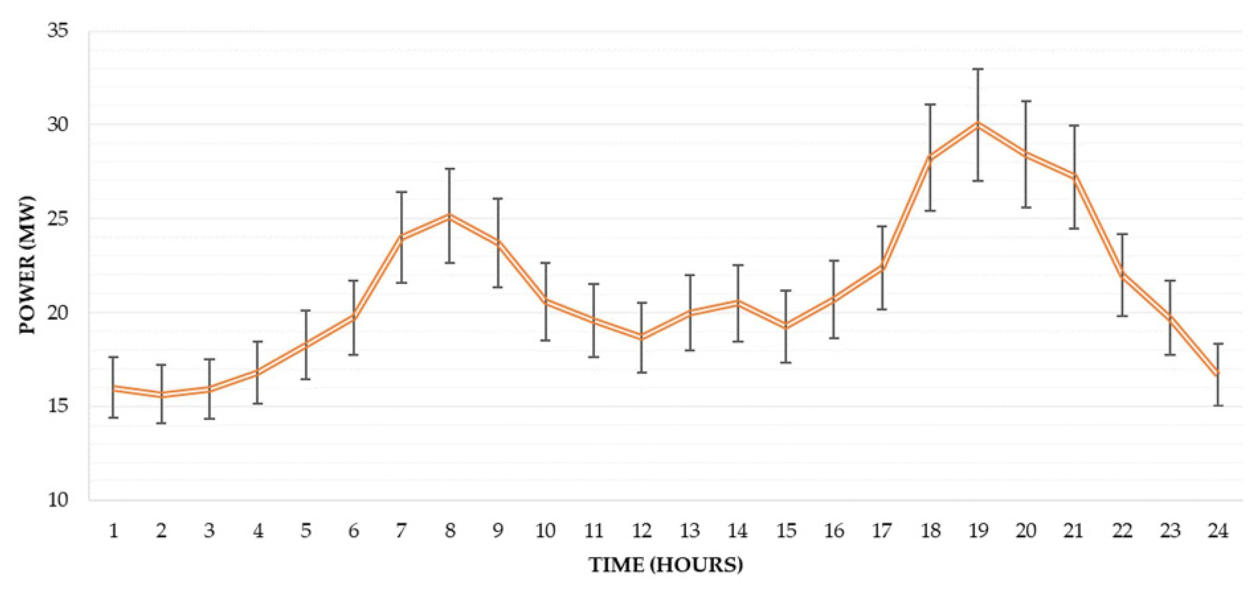
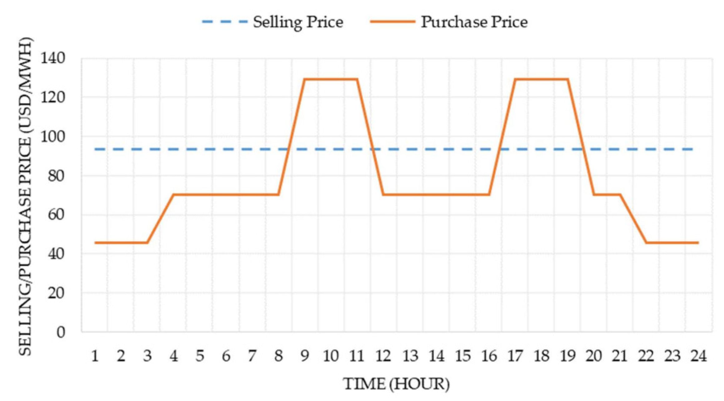
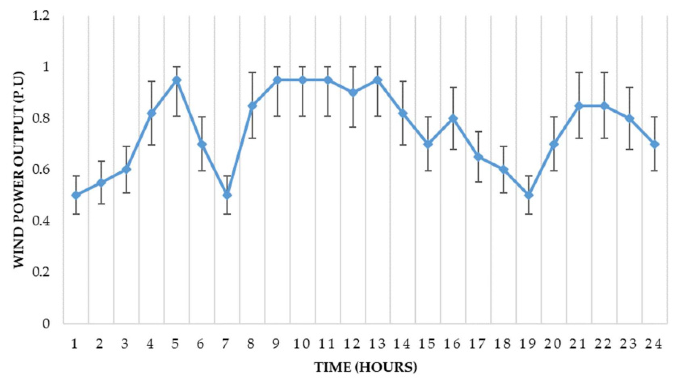
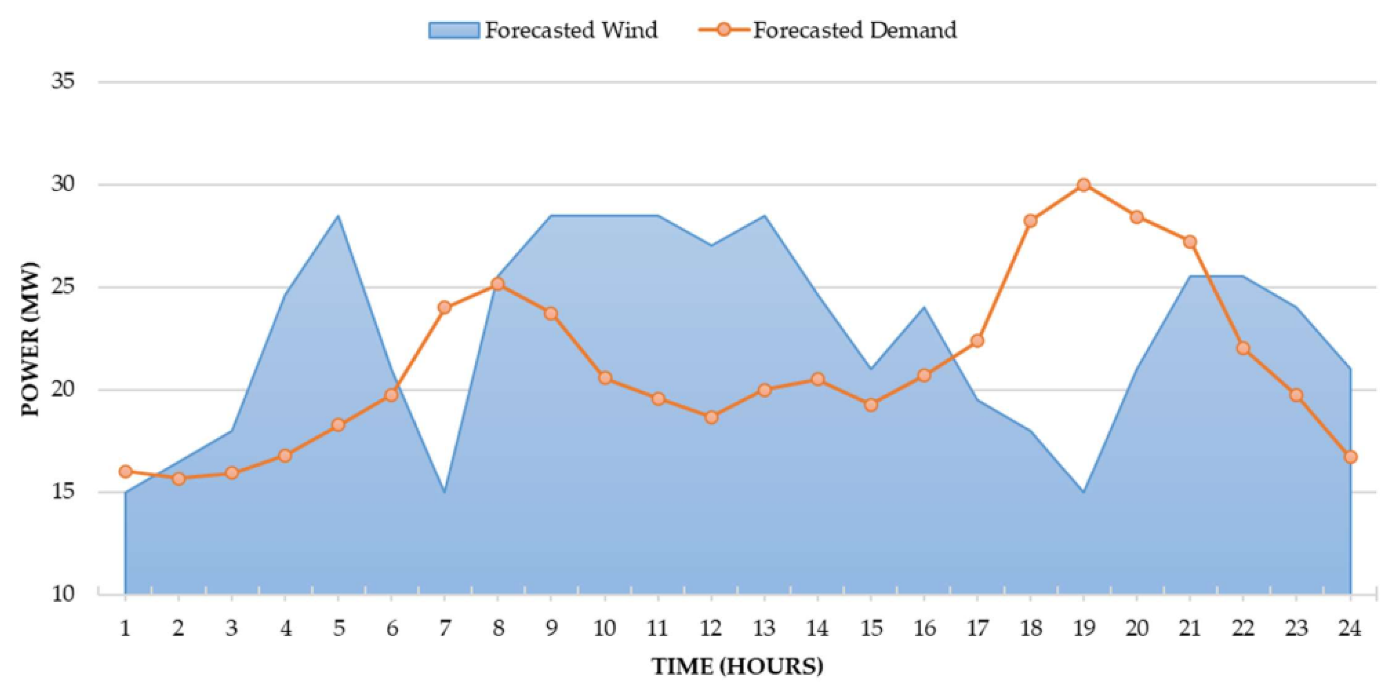
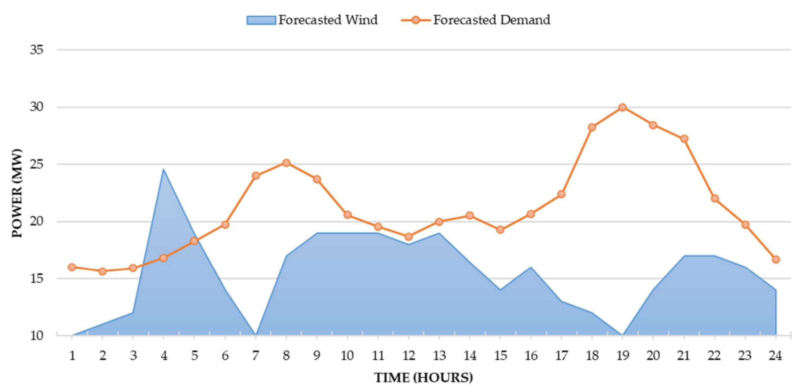
4.1. Study System

In this section, the proposed optimal model is implemented on a CVPP test system including RESs, battery storage systems, and residential consumers. Assuming that the CVPP test system is located in the Vietnamese power grid, this system uses the data collected from Vietnam’s electricity market, including wholesale tariff and typical wind, solar, and load profiles. In fact, the VPP model and a BC market have not been applied in Vietnam. However, with the rapid increase in RES sources, it is expected that this model will soon become relevant.

Until now, the Vietnamese government has had many policies to encourage renewable energy sources, especially solar energy. Accordingly, RESs are allowed to participate in the DA market at a preferential price of 83.8 USD per MWh [41]. In contrast, the electricity buying price in the wholesale market follows a three-tier tariff with peak-load, regular, and off-peak prices at 129.6 USD, 70.44 USD, and 45.65 USD per MWh, respectively (Figure 3) [42]. This tariff will be used in the proposed scheduling model. When a VPP enters the BC market, we assume that they can earn $8.38 for 1 MW of reserve capacity. Meanwhile, the price of each MWh of the activated reserve is 30% higher than the electricity selling price, i.e., 108.9 USD/MWh. The VPP must be able to generate a reserve power of at least 1 MW and maintain it for at least 3 h continuously.

In the VPP test system, the RESs are assumed to be wind power plants with the forecasted power curves of a wind generator (in p.u.) illustrated in Figure 4. Meanwhile, the battery storage systems can be treated as a large-scale storage system with technical data shown in

Table 2. Battery Storage System’s Technical Data.

Maximum/Minimum Energy Storage Limit (MWh)	20
Discharging/Charging Power (MW)	10
Charging Efficiency	90%

. The residential consumers have aggregated daily consumption equal to 510 MWh while their peak-load consumption can reach approximately 29 MW. Figure 5 describes the typical daily load considered as the long-term predictive data of consumers in this study.

To account for the uncertainty in demand and RES power output, the forecast errors are assumed as a normal distribution with a mean of zero and a standard deviation of 0.033 and 0.05, respectively, for demand and RESs power output. This means that the maximum errors described by the error bars in Figure 4 and Figure 5 are approximately 10% for demand and 15% for RESs power output. The risk level of probability constraints is assumed to be 5%.

The scheduling model is performed with the reserve activation probability in each hour generated from the uniform distribution function $U\left(0,0.05\right)$, so that the highest probability of reserve activation in every hour is 0.05. Furthermore, the impact of different aspects such as RESs power rating and ESSs capacity is also evaluated. The optimization problems are solved using CPLEX version 12.6 and the YALMIP toolbox [43] on a 64-bit core i5 1.9 GHz personal computer with 16 GB RAM.

4.2. Optimization Results

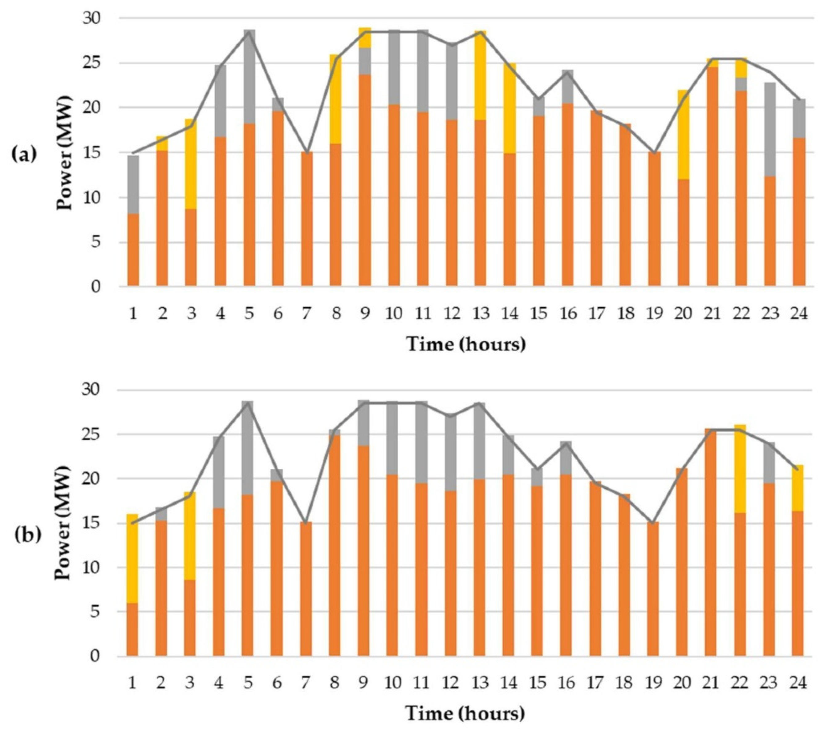
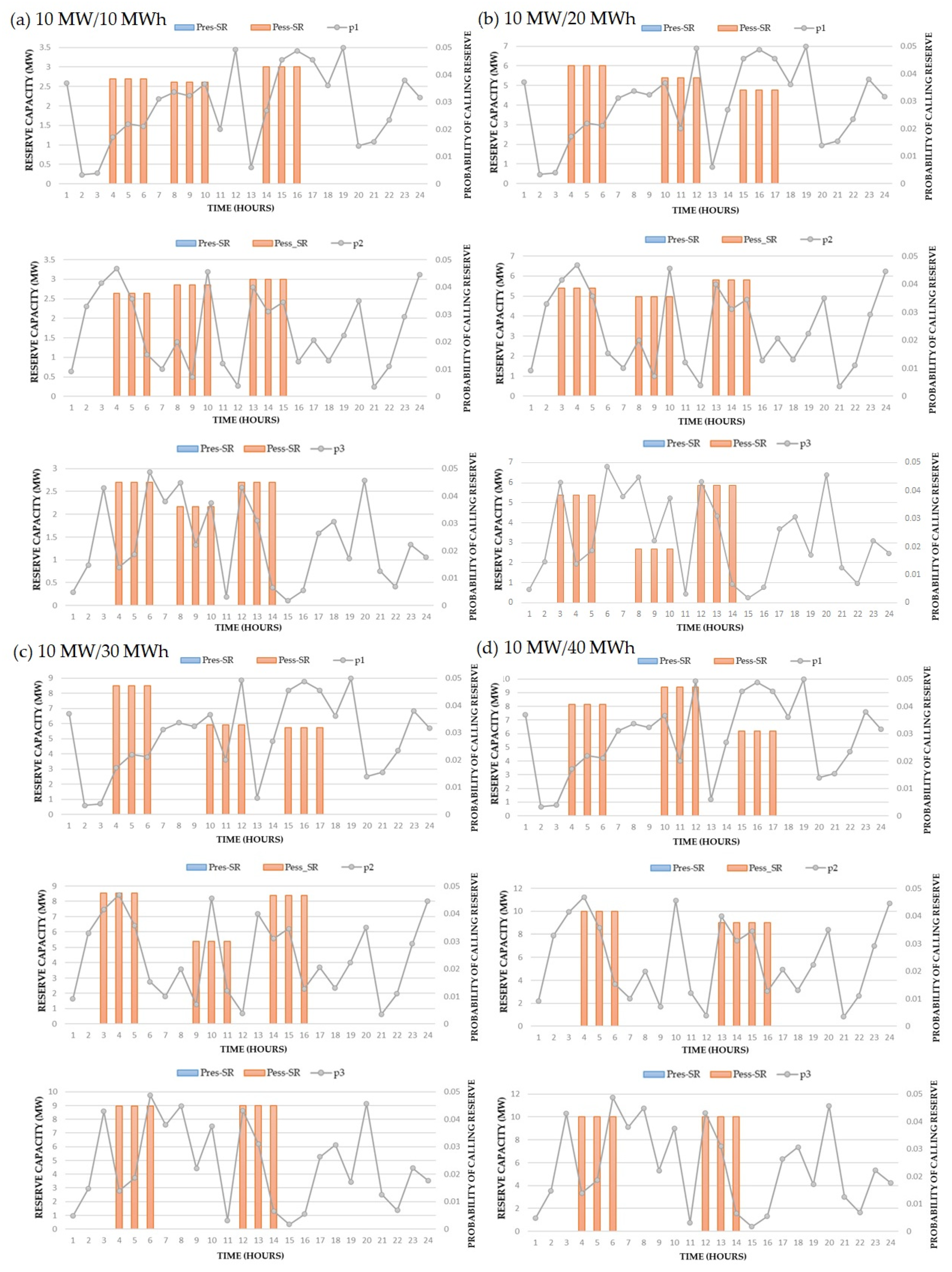
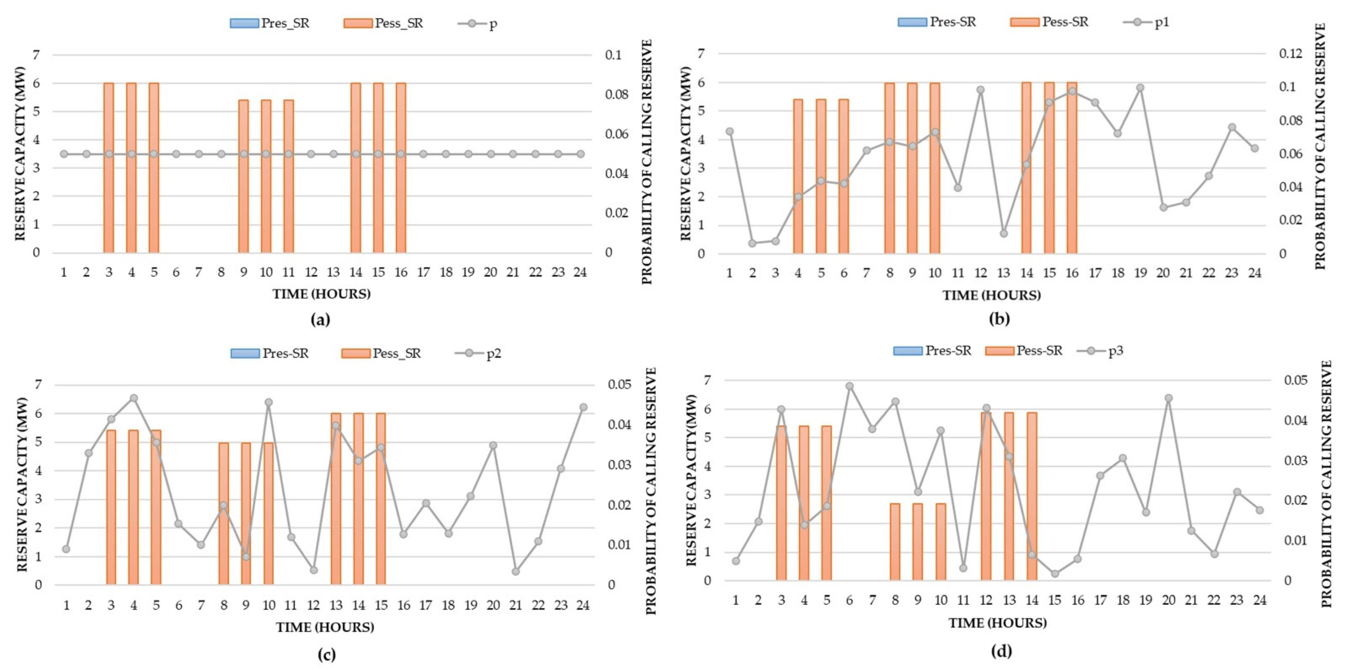
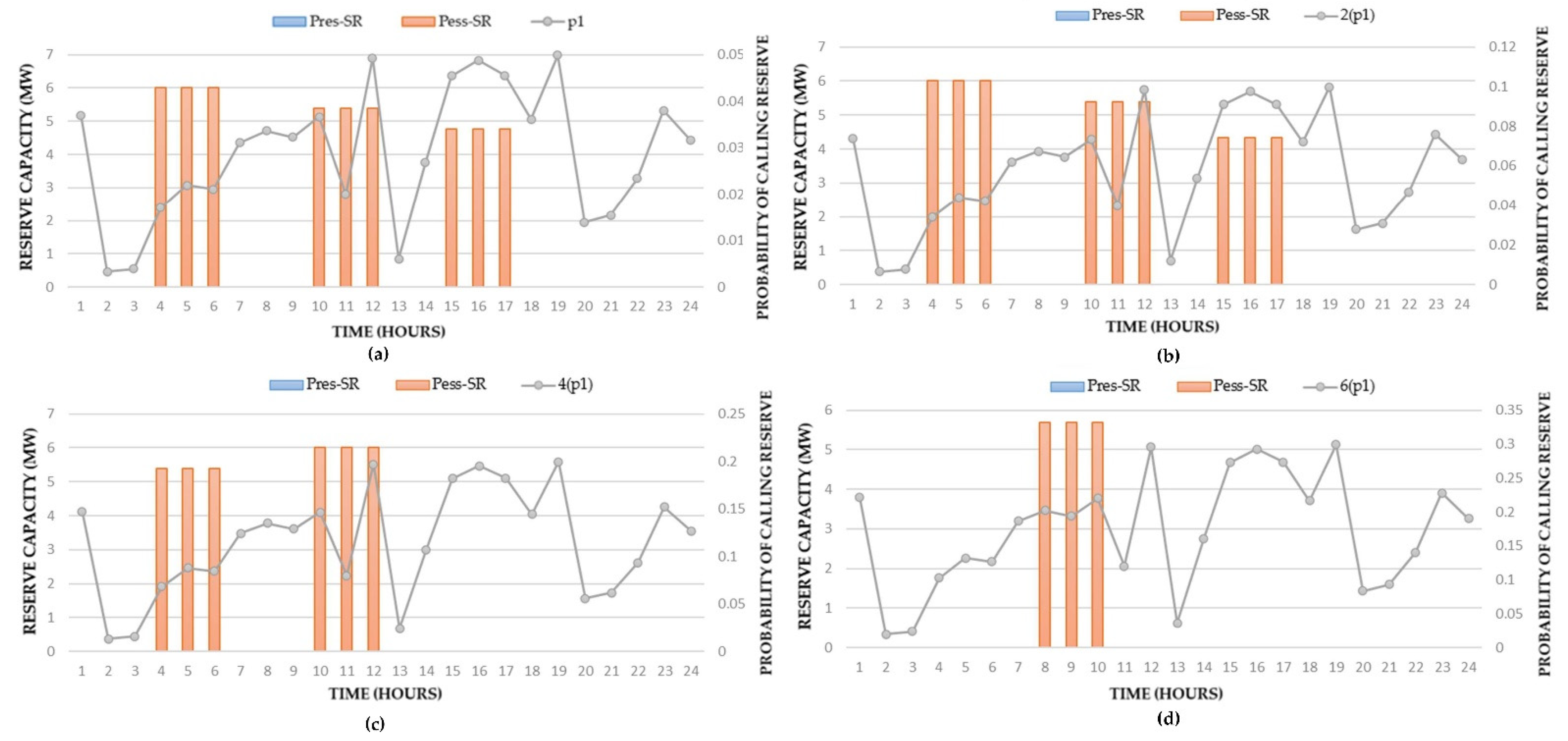
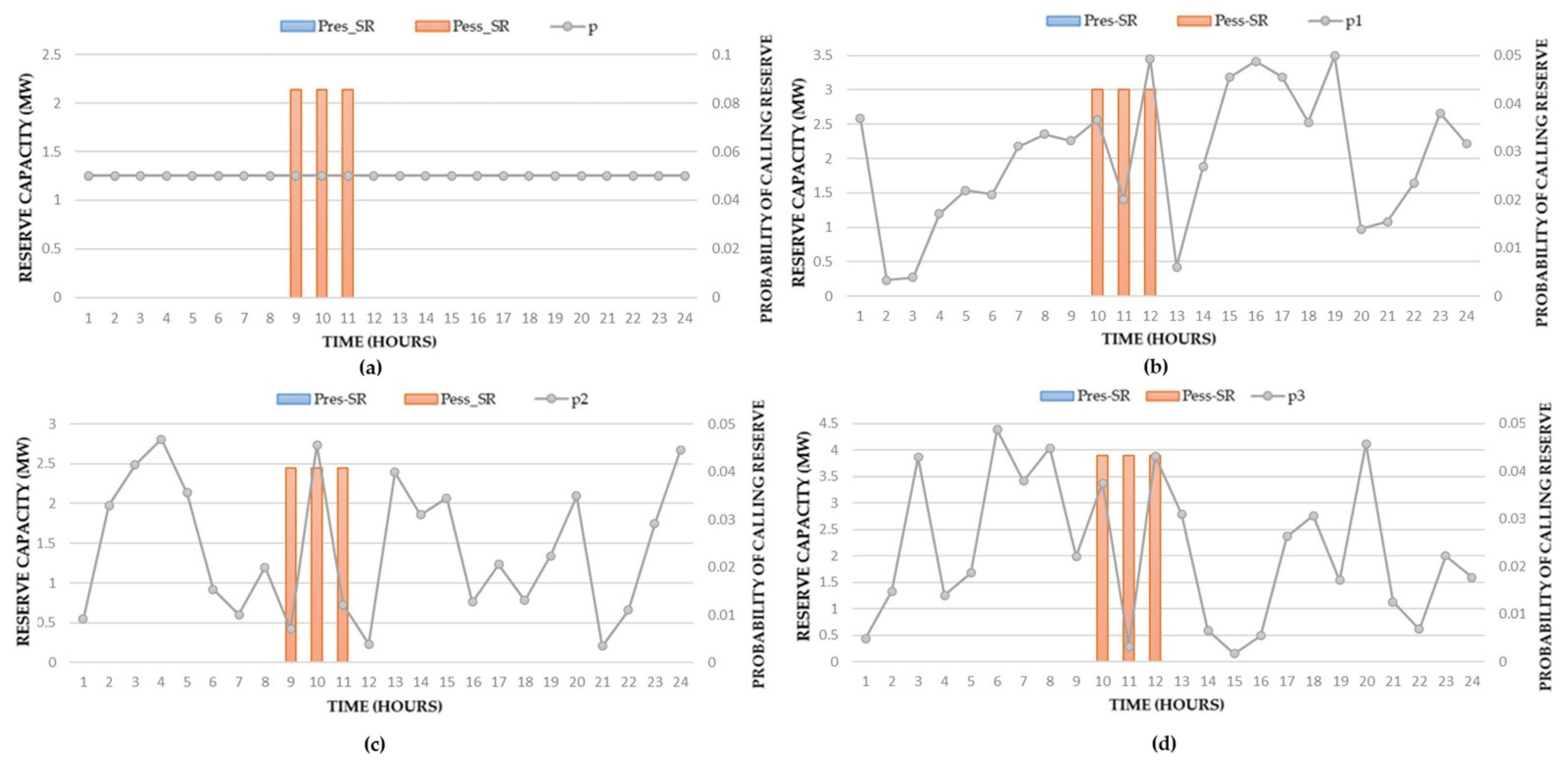
4.2.1. The Impact of the Reserve Activation Probability

With the wind farm’s aggregated capacity of 30 MW and the power curve (in p.u.) given in Section 4.1, we have the forecasted wind power and demand data presented in Figure 6. To evaluate the effect of the reserve activation probability on the VPP’s optimal schedule, we randomly generate three scenarios $p_1, p_2$, and $p_3$ of the reserve probability and apply them to the proposed model. Moreover, we consider a scenario with a reserve activation probability of 0.05 for all hours to see the effect of this uncertain parameter on the optimal results. The VPP’s optimal reserve capacity corresponding to each scenario is presented in Figure 7. It can be seen that the ESS provides all the reserve capacity.

Figure 6 shows that the wind farm’s available power output from hour 3 to hour 5, hour 9 to hour 16, and hour 22 to hour 24 is relatively higher than the demand. Therefore, it is clear that the VPP can provide reserve service during these periods; on the contrary, this service is unlikely to be available during the rest of the day. Figure 7a shows the VPP’s optimal reserve contract if the probability of reserve activation is 0.05 for every hour. It can be seen that the VPP only provides reserve service when the power output of RES is redundant.

By contrast, the optimal results in the scenario $p_1$ show that the VPP’s reserve service is available in hours 6 and 17 while wind power is equal to or even less than the demand (Figure 7b). This is due to the high probability of calling reserve during these hours. Note that the main role of ESS is to store the excess energy of RES or buy low-priced electricity from the network; then the ESS energy will be discharged to provide reserve or supply the load when the RES’ power output is low and avoid the VPP having to buy electricity at a high price from the system. It is easy to see that the VPP provides a reserve service when the RES power output is not high enough will to cause the VPP to reduce the selling power or buy more electricity at other times to recharge ESS. This means that the probabilities of calling reserve in hours 6 and 17 are high enough so that the VPP expects the profit obtained from the BC market will be greater than the profit decline in the energy market. The optimal results in scenarios 2 and 3 also show the same thing. Even in scenario 3, the wind power in hours 15 and 16 is higher than the load by approximately the minimum threshold $S{R}_{min}$, but VPP still decide not to provide reserve service during these hours due to the very small probability of calling reserve (less than 1%) (Figure 7d).

As discussed in Section 2, the energy trading scheme during the period without reserve contract is assumed to be adjustable in the intraday market to utilize the RES available power output and maximize the VPP profit. This adjustment is not allowed to affect the performance of the reserve contract next period, even in an extreme case. Figure 8 shows the energy trade between the VPP and the main grid in scenario $p_1$ for two extreme cases: (a) the full reserve capacity is called and generated for the entire contract duration, and (b) the reserve capacity is not called and generated. Similarly, the operating plans of ESS and RES corresponding to two cases are described in Figure 9 and Figure 10, respectively. In the proposed model, VPP selling/buying energy and the operating parameters of ESS and RES in each hour are second-stage variables considering the uncertain nature of RESs and demand. Therefore, the results can be treated as predictions of future trading plans with the mean value and the fluctuation range represented by bar charts and error bars, respectively. For simplicity, Figure 9 and Figure 10 show only the mean value of the obtained results.

It is clear that with a relatively small probability of reserve activation, the energy trading scheme in Figure 8b can be applied in the DA market. Meanwhile, Figure 8a shows that the VPP’s highest adjustment in the intraday market if the reserve capacity is fully called and generated during the entire contract period. On the other hand, the ESS provides all reserve capacity; therefore, the ESS energy is maintained at the maximum level during the contract period to be available for reserve provisioning (Figure 9b). After each provisioning period of the reserve, the VPP’s adjustment should bring the ESS’s energy back to its maximum level just before the next reserve period (Figure 9a). This is still necessary even if the actual provisioning level is lower than the extreme case in this paper. Moreover, Figure 10 shows that the RES power output is fully utilized in both cases of providing reserve.

Table 3. The VPP’s optimal profit.

Scenario	No Reserve	$\mathit{p} = 0.05$	${\mathit{p}}_1$	${\mathit{p}}_2$	${\mathit{p}}_3$
The optimal profit (USD)	3548	4134	4168	4230	4499

shows the optimal profit of the VPP corresponding to each scenario of $p$and compares them with the case where VPP does not participate in the BC market. It is easy to see that the VPP becomes more profitable when entering the BC market because reserve energy is 30% higher than the wholesale price. Even if the reserve capacity is not activated, they still profit from the provision of reserve capacity. Paying attention to the difference between the reserve activation probabilities during the hours helps the VPP sell reserve at the higher probability hours, thereby earning a higher profit.

Next, the change of the optimal results as the probability of contingencies increases or decreases is evaluated. Note that in the above section, we assume that the maximum probability of active reserve is 0.05. However, in practice, depending on the penetration level of the RESs in the power system, this probability may be higher. Figure 11 shows the VPP’s optimal reserve capacity if the reserve activation probabilities in scenario $p_1$are multiplied by two, four, and six times, corresponding to the maximum value of 0.1, 0.2, and 0.3. It can be seen that, as the reserve activation probability increases, the number of hours that the VPP can provide the reserve service decreases. It seems that the VPP expects to profit from the provision of reserve control rather than from the actual reserve energy called and generated. This can be explained because RES power output is not enough to supply the load, especially in the period from hour 17 to hour 21, so that the ESS needs to provide a part of the load. An activated reserve contract period will use most of the ESS energy so that the VPP must purchase electricity from the main grid (hour 18 in Figure 8a and Figure 9a). However, the peak-load price of 129.6 USD/MWh is higher than the total reserve capacity and reserve energy price; consequently, the operating cost increases.

4.2.2. The Impact of the RES Sizing

This section tests the VPP model with the wind farm’s maximum available power output of 20 MW. With the power curve (in p.u) given in Section 4.1, we have the forecasted wind and load capacity shown in Figure 12. It is easy to see that the wind capacity is not enough to supply the load most of the time. Therefore, ESS needs to increase the purchase of electricity with the off-peak price to store and provide to the local load during the peak-load period instead of focusing on reserve service. As a result, the reserve capacity and the number of hours of reserve service decreases, and the value of the reserve activation probability each hour has little effect on the optimal results (Figure 13). Note that we are only interested in the VPP’s ability to provide reserve service when the RES power output is even less than the local load in this section. If the RES power output during most hours of the day is higher than the load, deciding whether to enter the BC market or not becomes much simpler.

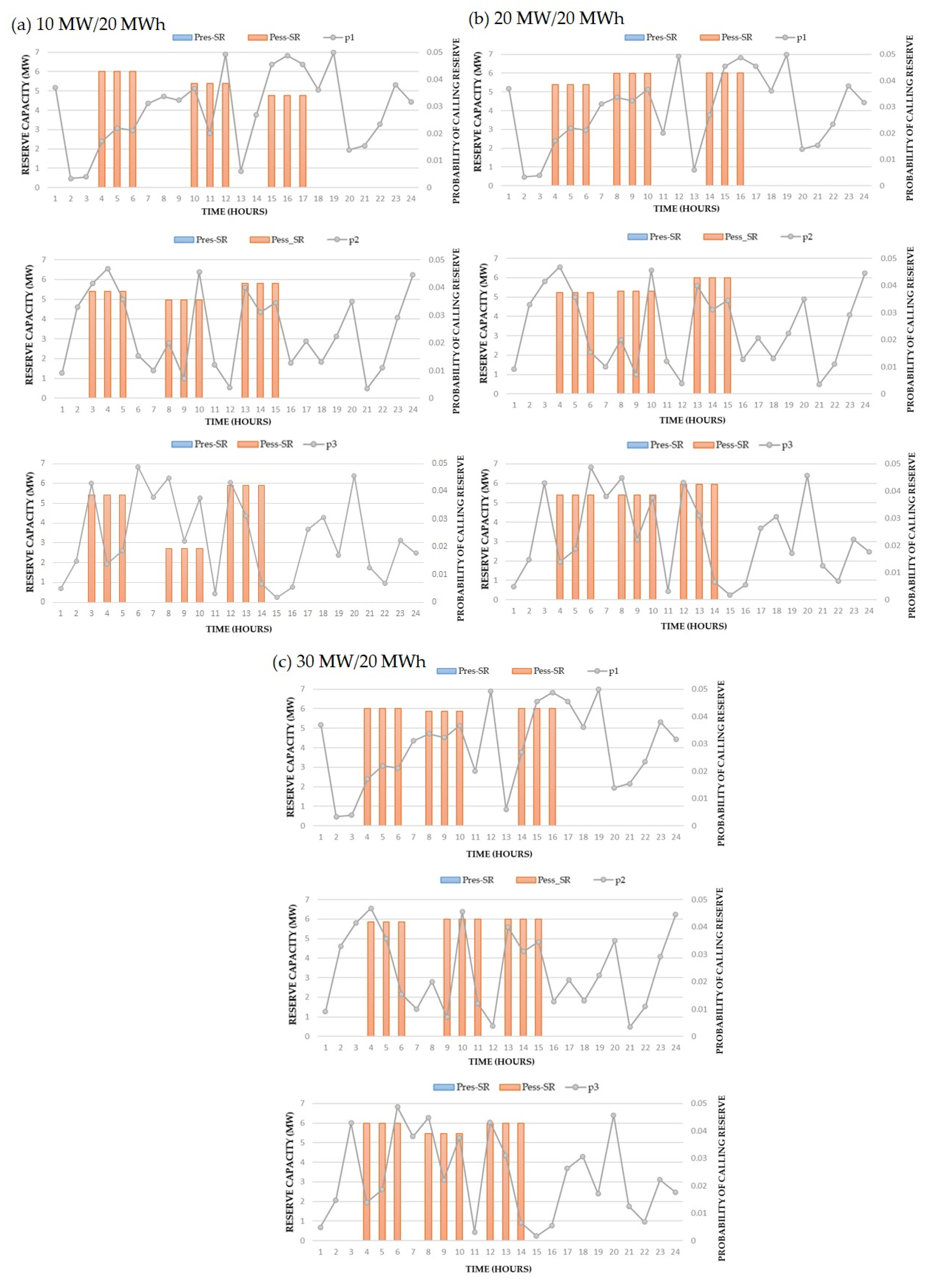
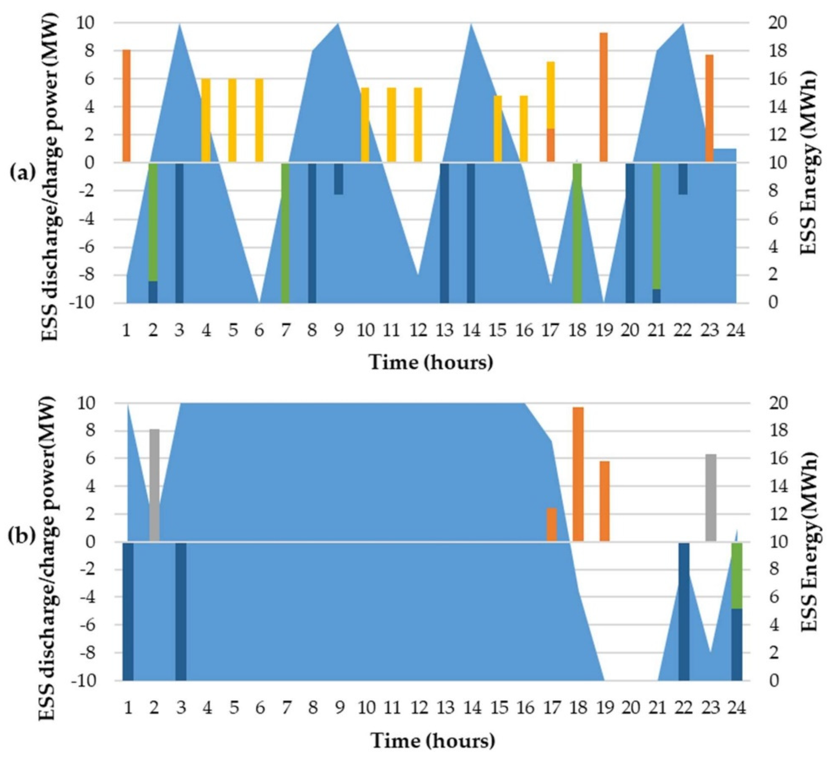
4.2.3. The Impact of the ESS Sizing

In this section, we consider the effect of the ESS sizing on the VPP’s optimal reserve capacity. Figure 14 and Figure 15 show the optimal reserve contract of the VPP for three scenarios of reserve activation probability and several ESS sizing. It can be seen that when the rated capacity of the ESS is 20 MWh, and the rated power varies from 10 MW to 30 MW, the obtained results show that the rated power of the ESS does not affect the optimal reserve sizing much. Meanwhile, when the ESS rated power is 10 MW and the rated capacity increases from 10 MW to 40 MW, the optimal reserve capacity also increases for all three scenarios of the reserve probability. However, while the scenario $p_1$ still maintains three contract periods, the number of provisioning periods in scenarios $p_2$ and $p_3$ decreases, and the reserve capacity in each period increase significantly. It can be explained that in scenario $p_1$, most of hours with a high probability of reserve activation also have a relatively high RES power output. By contrast, in scenarios $p_2$ and $p_3$, there are some hours of high RES power output but low probability of reserve activation, so that the high rated capacity of ESS will help VPP to accumulate energy to provide higher reserve capacity during high-probability hours.

5. Conclusions

This paper considers and analyzes the VPP’s optimal scheduling problem in the BC and energy markets. The main purpose is determining the VPP optimal reserve sizing and the possible operating scenarios of the VPP in the DA and ID markets. This task is challenging because the VPP operators do not know whether their reserve service will be called; hence, the profit from provisioning reserve service is uncertain. To solve this problem, we build a two-stage chance-constrained model considering the probability of reserve activation. The uncertainty in the load and the RES maximum power output is also taken into account. The influence of reserve activation probability, RES capacity, and ESS sizing on optimal reserve capacity is studied and analyzed.

The results show that paying attention to the hourly reserve probability will help schedule the operation of the VPP to provide redundancy at times of high reserve activation probability. The results also show that the reserve provisioning duration decreases if the reserve probability increases with the given input parameters. From that, it can be seen that the VPP expects to make a profit from reserve capacity provision than from the actual reserve energy generated. Furthermore, ESS plays a significant role in providing reserve, helping the VPP provide reserve even in the shortage of power output.

The proposed approach can be applied to any VPP models with different types of RES or controllable loads. Moreover, the model can be readily adapted to study the influence of other factors, such as the reserve activation price. There are some limitations to the proposed model. For example, the demand response, which can be treated as a reserve in the peak-load periods, was not accounted for. These topics are left for future work.

References

1. Arias, J. Solar Energy, Energy Storage and Virtual Power Plants in Japan. Available online: https://www.eu-japan.eu/sites/default/files/publications/docs/min18_1_arias_solarenergy-energystorageandvirtualpowerplantsinjapan.pdf (accessed on 18 September 2021).
2. Wassermann, S.; Reeg, M.; Nienhaus, K. Current challenges of Germany’s energy transition project and competing strategies of challengers and incumbents: The case of direct marketing of electricity from renewable energy sources. Energy Policy 2015, 76, 66–75. [Google Scholar] [CrossRef]
3. Neme, C.; Energy Futures Group; Cowart, R.; Regulator Assistance Project. Energy Efficiency Participation in Electricity Capacity Markets—The US Experience; Regulator Assistance Project: Montpelier, VT, USA, 2014. [Google Scholar]
4. Oureilidis, K.; Malamaki, K.N.; Gallos, K.; Tsitsimelis, A.; Dikaiakos, C.; Gkavanoudis, S.; Cvetkovic, M.; Mauricio, J.M.; Ortega, J.M.M.; Ramos, J.L.M.; et al. Ancillary services market design in distribution networks: Review and identification of barriers. Energies 2020, 13, 917. [Google Scholar] [CrossRef] [Green Version]
5. Helman, U. Distributed energy resources in the US wholesale markets: Recent trends, new models, and forecasts. In Consumer, Prosumer, Prosumager: How Service Innovations Will Disrupt the Utility Business Model; Academic Press/Elsevier: San Diego, CA, USA, 2019; pp. 431–469. ISBN 9780128168356. [Google Scholar]
6. IRENA. Redesigning Capacity Markets: Innovation Landscape Brief; International Renewable Energy Agency: Abu Dhabi, United Arab Emirates, 2019; ISBN 978-92-9260-130-0. [Google Scholar]
7. Bai, H.; Miao, S.; Ran, X.; Ye, C.; Bai, H.; Miao, S.; Ran, X.; Ye, C. Optimal Dispatch Strategy of a Virtual Power Plant Containing Battery Switch Stations in a Unified Electricity Market. Energies 2015, 8, 2268–2289. [Google Scholar] [CrossRef] [Green Version]
8. Mashhour, E.; Moghaddas-Tafreshi, S.M. Bidding Strategy of Virtual Power Plant for Participating in Energy and Spinning Reserve Markets—Part I: Problem Formulation. IEEE Trans. Power Syst. 2011, 26, 949–956. [Google Scholar] [CrossRef]
9. Pudjianto, D.; Ramsay, C.; Strbac, G. Microgrids and virtual power plants: Concepts to support the integration of distributed energy resources. Proc. Inst. Mech. Eng. Part A J. Power Energy 2008, 222, 731–741. [Google Scholar] [CrossRef]
10. Sikorski, T.; Jasiński, M.; Ropuszyńska-Surma, E.; Węglarz, M.; Kaczorowska, D.; Kostyła, P.; Leonowicz, Z.; Lis, R.; Rezmer, J.; Rojewski, W.; et al. A Case Study on Distributed Energy Resources and Energy-Storage Systems in a Virtual Power Plant Concept: Economic Aspects. Energies 2019, 12, 4447. [Google Scholar] [CrossRef] [Green Version]
11. Pudjianto, D.; Ramsay, C.; Strbac, G. Virtual power plant and system integration of distributed energy resources. IET Renew. Power Gener. 2007, 1, 10–16. [Google Scholar] [CrossRef]
12. Naval, N.; Yusta, J.M. Virtual power plant models and electricity markets—A review. Renew. Sustain. Energy Rev. 2021, 149, 111393. [Google Scholar] [CrossRef]
13. Rahimiyan, M.; Baringo, L. Strategic Bidding for a Virtual Power Plant in the Day-Ahead and Real-Time Markets: A Price-Taker Robust Optimization Approach. IEEE Trans. Power Syst. 2016, 31, 2676–2687. [Google Scholar] [CrossRef]
14. Gazijahani, F.S.; Salehi, J. IGDT-Based Complementarity Approach for Dealing with Strategic Decision Making of Price-Maker VPP Considering Demand Flexibility. IEEE Trans. Ind. Inform. 2020, 16, 2212–2220. [Google Scholar] [CrossRef]
15. Koraki, D.; Strunz, K. Wind and solar power integration in electricity markets and distribution networks through service-centric virtual power plants. IEEE Trans. Power Syst. 2018, 33, 473–485. [Google Scholar] [CrossRef]
16. Zhao, Q.; Shen, Y.; Li, M. Control and Bidding Strategy for Virtual Power Plants with Renewable Generation and Inelastic Demand in Electricity Markets. IEEE Trans. Sustain. Energy 2016, 7, 562–575. [Google Scholar] [CrossRef]
17. Baringo, A.; Baringo, L.; Arroyo, J.M. Day-Ahead Self-Scheduling of a Virtual Power Plant in Energy and Reserve Electricity Markets under Uncertainty. IEEE Trans. Power Syst. 2019, 34, 1881–1894. [Google Scholar] [CrossRef]
18. Mazzi, N.; Trivella, A.; Morales, J.M. Enabling active/passive electricity trading in dual-price balancing markets. IEEE Trans. Power Syst. 2019, 34, 1980–1990. [Google Scholar] [CrossRef] [Green Version]
19. Nguyen, H.T.; Le, L.B.; Wang, Z. A Bidding Strategy for Virtual Power Plants with the Intraday Demand Response Exchange Market Using the Stochastic Programming. IEEE Trans. Ind. Appl. 2018, 54, 3044–3055. [Google Scholar] [CrossRef]
20. Dabbagh, S.R.; Sheikh-El-Eslami, M.K. Risk Assessment of Virtual Power Plants Offering in Energy and Reserve Markets. IEEE Trans. Power Syst. 2016, 31, 3572–3582. [Google Scholar] [CrossRef]
21. Vahedipour-Dahraie, M.; Rashidizade-Kermani, H.; Shafie-khah, M.; Catalao, J.P.S. Risk-Averse Optimal Energy and Reserve Scheduling for Virtual Power Plants Incorporating Demand Response Programs. IEEE Trans. Smart Grid 2020, 1. [Google Scholar] [CrossRef]
22. Zhou, Y.; Wei, Z.; Sun, G.; Cheung, K.W.; Zang, H.; Chen, S. Four-level robust model for a virtual power plant in energy and reserve markets. IET Gener. Transm. Distrib. 2019, 13, 2006–2014. [Google Scholar] [CrossRef]
23. Ocker, F.; Braun, S.; Will, C. Design of European balancing power markets. Int. Conf. Eur. Energy Mark. EEM 2016. [Google Scholar] [CrossRef] [Green Version]
24. Poplavskaya, K.; Lago, J.; de Vries, L. Effect of market design on strategic bidding behavior: Model-based analysis of European electricity balancing markets. Appl. Energy 2020, 270, 115130. [Google Scholar] [CrossRef]
25. Hayashi, K.; Mikami, Y.; Hirano, K.; Terayama, H. Development of Large-Scale Hybrid Power Storage System: System Demonstration Project in Lower Saxony, Germany: Hitachi Review. Available online: http://www.hitachi.com/rev/archive/2020/r2020_04/04c02/index.html (accessed on 18 September 2021).
26. Bouffard, F.; Galiana, F.D. An Electricity Market with a Probabilistic Spinning Reserve Criterion. IEEE Trans. Power Syst. 2004, 19, 300–307. [Google Scholar] [CrossRef]
27. Bruninx, K.; Delarue, E. Endogenous Probabilistic Reserve Sizing and Allocation in Unit Commitment Models: Cost-Effective, Reliable, and Fast. IEEE Trans. Power Syst. 2017, 32, 2593–2603. [Google Scholar] [CrossRef]
28. Tahanan, M.; van Ackooij, W.; Frangioni, A.; Lacalandra, F. Large-scale Unit Commitment under uncertainty. 4OR 2015, 13, 115–171. [Google Scholar] [CrossRef] [Green Version]
29. Pagnoncelli, B.K.; Ahmed, S.; Shapiro, A.; Ahmed, S.; Shapiro, A. Sample Average Approximation Method for Chance Constrained Programming: Theory and Applications. J. Optim. Theory Appl. 2009, 142, 399–416. [Google Scholar] [CrossRef] [Green Version]
30. Wang, Q.; Guan, Y.; Wang, J. A chance-constrained two-stage stochastic program for unit commitment with uncertain wind power output. IEEE Trans. Power Syst. 2012, 27, 206–215. [Google Scholar] [CrossRef]
31. Basciftci, B.; Ahmed, S.; Gebraeel, N.Z.; Yildirim, M. Stochastic optimization of maintenance and operations schedules under unexpected failures. IEEE Trans. Power Syst. 2018, 33, 6755–6765. [Google Scholar] [CrossRef]
32. Yang, X.; Xu, C.; He, H.; Yao, W.; Wen, J.; Zhang, Y. Flexibility Provisions in Active Distribution Networks with Uncertainties. IEEE Trans. Sustain. Energy 2021, 12, 553–567. [Google Scholar] [CrossRef]
33. AEMO Emerging Generation and Energy Storage in the NEM. Available online: https://aemo.com.au/-/media/files/electricity/nem/initiatives/emerging-generation/eges_stakeholder_paper_final.pdf?la=en&hash=5E82D40582C56B34327D120A366EF044 (accessed on 12 October 2021).
34. IRENA. Electricity Storage Valuation Framework: Assessing System Value and Ensuring Project Viability; International Renewable Energy Agency: Abu Dhabi, United Arab Emirates, 2020; ISBN 978-92-9260-161-4. [Google Scholar]
35. FINGRID. Reserve Products and Reserve Market Places. Available online: https://www.fingrid.fi/globalassets/dokumentit/en/electricity-market/reserves/reserve-products-and-reserve-market-places.pdf (accessed on 18 September 2021).
36. Yamin, H.Y. Spinning reserve uncertainty in day-ahead competitive electricity markets for GENCOs. IEEE Trans. Power Syst. 2005, 20, 521–523. [Google Scholar] [CrossRef]
37. Zhang, L.; Yuan, Y.; Yuan, X.; Chen, B.; Su, D.; Li, Q. Spinning Reserve Requirements Optimization Based on an Improved Multiscenario Risk Analysis Method. Math. Probl. Eng. 2017, 2017. [Google Scholar] [CrossRef] [Green Version]
38. Wang, M.Q.; Yang, M.; Liu, Y.; Han, X.S.; Wu, Q. Optimizing probabilistic spinning reserve by an umbrella contingencies constrained unit commitment. Int. J. Electr. Power Energy Syst. 2019, 109, 187–197. [Google Scholar] [CrossRef]
39. Toubeau, J.F.; Bottieau, J.; De Greeve, Z.; Vallee, F.; Bruninx, K. Data-Driven Scheduling of Energy Storage in Day-Ahead Energy and Reserve Markets with Probabilistic Guarantees on Real-Time Delivery. IEEE Trans. Power Syst. 2021, 36, 2815–2828. [Google Scholar] [CrossRef]
40. Ahmed, S.; Shapiro, A.; Stewart, H.M. Solving Chance-Constrained Stochastic Programs via Sampling and Integer Programming. In State-of-the-Art Decision-Making Tools in the Information-Intensive Age; Informs: Catonsville, MD, USA, 2008. [Google Scholar] [CrossRef] [Green Version]
41. EVN. The Price of Rooftop Solar Power after June 30, 2019 is 1,943 VND/kWh. Available online: https://www.evn.com.vn/d6/news/Gia-dien-mat-troi-mai-nha-sau-thoi-diem-3062019-la-1943-dongkWh-6-12-25351.aspx (accessed on 18 September 2021).
42. EVN. Electricity Tariff in the Wholesale Market. Available online: https://www.evn.com.vn/c3/evn-va-khach-hang/Bieu-gia-ban-buon-dien-9-80.aspx (accessed on 18 September 2019).
43. Löfberg, J. YALMIP: A toolbox for modeling and optimization in MATLAB. Proc. IEEE Int. Symp. Comput. Control Syst. Des. 2004, 284–289. [Google Scholar] [CrossRef]
Figure 1. The structure of the VPP.
Applsci 11 09717 g001
Figure 2. The VPP scheduling strategy in BC, DA, and ID markets.
Applsci 11 09717 g002
Figure 3. The selling/buying price in the DA market.
Applsci 11 09717 g003
Figure 4. The forecasted wind power curve in p.u.
Applsci 11 09717 g004
Figure 5. Forecasted Demand.
Applsci 11 09717 g005
Figure 6. Forecasted wind power and demand.
Applsci 11 09717 g006
Figure 7. The VPP’s reserve bidding with (a) p = 0.05 for all hours, (b) scenario p 1 , (c) scenario p 2   , and (d) scenario p 3   of the reserve probability.
Applsci 11 09717 g007
Figure 8. The VPP’s selling/buying power with scenario p 1   of the reserve probability: (a) The reserve bid is called on to produce; (b) the reserve bid is not called on to produce.
Applsci 11 09717 g008
Figure 9. The ESS operational scheduling with scenario p 1   of the reserve probability: (a) The reserve bid is called on to produce; (b) the reserve bid is not called on to produce.
Applsci 11 09717 g009
Figure 10. The RES operational scheduling with scenario p 1   of the reserve probability: (a) The reserve bid is called on to produce; (b) the reserve bid is not called on to produce.
Applsci 11 09717 g010
Figure 11. The VPP’s reserve bidding with reserve probability (a) p 1 , (b) 2 p 1 , (c) 4 p 1   , (d) 6 p 1   .
Applsci 11 09717 g011
Figure 12. Forecasted wind power and demand with RES’ maximum power output of 20 MW.
Applsci 11 09717 g012
Figure 13. The VPP’s reserve bidding with reserve probability: (a) p = 0.05 for all hours, (b) scenario p 1 , (c) scenario p 2 , and (d) scenario p 3   with RES’ maximum power output of 20 MW.
Applsci 11 09717 g013
Figure 14. VPP’s reserve capacity for different ESS power ratings and reserve probability scenarios.
Applsci 11 09717 g014
Figure 15. The VPP’s reserve bidding with different ESS capacity and reserve probability scenarios.
Applsci 11 09717 g015