Article

A Bayesian Modeling Approach to Situated Design of Personalized Soundscaping Algorithms

1
Department of Electrical Engineering, Eindhoven University of Technology, 5612 AP Eindhoven, The Netherlands
2
GN Hearing, 5612 AB Eindhoven, The Netherlands
*
Author to whom correspondence should be addressed.
Appl. Sci. 2021, 11(20), 9535; https://doi.org/10.3390/app11209535
Submission received: 13 August 2021 / Revised: 5 October 2021 / Accepted: 8 October 2021 / Published: 14 October 2021
(This article belongs to the Special Issue AI, Machine Learning and Deep Learning in Signal Processing)

Abstract

:
Effective noise reduction and speech enhancement algorithms have great potential to enhance lives of hearing aid users by restoring speech intelligibility. An open problem in today’s commercial hearing aids is how to take into account users’ preferences, indicating which acoustic sources should be suppressed or enhanced, since they are not only user-specific but also depend on many situational factors. In this paper, we develop a fully probabilistic approach to “situated soundscaping”, which aims at enabling users to make on-the-spot (“situated”) decisions about the enhancement or suppression of individual acoustic sources. The approach rests on a compact generative probabilistic model for acoustic signals. In this framework, all signal processing tasks (source modeling, source separation and soundscaping) are framed as automatable probabilistic inference tasks. These tasks can be efficiently executed using message passing-based inference on factor graphs. Since all signal processing tasks are automatable, the approach supports fast future model design cycles in an effort to reach commercializable performance levels. The presented results show promising performance in terms of SNR, PESQ and STOI improvements in a situated setting.

1. Introduction

The ideal noise reduction or speech enhancement algorithm depends on the lifestyle and living environment of the hearing aid user. Therefore, personalization of these algorithms is very difficult to achieve in advance. Even if a preliminary design of these personalized algorithms were possible, unforeseen events can still degrade the performance of the pre-trained noise reduction algorithms. Hence there is a need for algorithms that users can easily customize according to the situation they are in. Consider the situation in which you are having a conversation at a party, where an arriving group of guests disrupts the conversation with their chatter. When a hearing aid’s noise reduction algorithm fails to perform well under these conditions, it would be desirable to let the user record on the spot a short segment of the background chatter and instantly design an algorithm that uses the characteristics of the recorded signal to better suppress similar background noise signals during the ongoing conversation. In this paper, we call this on-the-spot user-driven algorithm design process “situated soundscaping”, where a user can generate her own noise reduction algorithm on the spot and shape her perceived acoustic environment (“soundscaping”) by adjusting source-specific gains according to her preferences.
Situated design of hearing aid algorithms has drawn interest of the research community before. For instance, Reddy et al. [1] proposed to include trade-off parameters in their noise reduction algorithm to allow users to find a compromise between noise reduction and speech distortion. This mechanism, however, only allows users to alter the influence of the noise reduction algorithm post-hoc, rather than to support situated design of the noise reduction algorithm itself. In contrast, our proposed approach is based on source separation and allows users to fully personalize the algorithm under in-the-field conditions. The field of source separation can be subdivided into two groups. One research thread is based on blind source separation methods (BSS) for acoustic signals [2,3,4,5], which is commonly implemented by only assuming statistical independence between the different source signals and by optimizing for a selected independence metric. Unfortunately, the performance and computational costs of real-time BSS are not adequate for hearing aid applications. Rather we would like to help these algorithms in separating the sources by providing additional information of the sources in the mixture. In contrast to blind source separation, informed source separation (ISS) methods use significant prior information about the observed signals [6]. ISS technology for audio signals typically use log-power domain models [7,8,9]. An issue with log-power domain models is that they contain an intractable signal mixing model [10] that is commonly approximated by the max-model [11] which leads to perceivable artifacts due to time-frequency masking [12]. Furthermore, this technique is commonly extended with non-negative matrix factorization (NMF) [13,14,15] for improved performance. On the interface of blind and informed source separation in a probabilistic context recently new works have been published. In [16] a blind signal separation algorithm is presented, based on earlier works in [17,18,19]. Here the individual signals are represented by state space models with a sparse input. Their approach allows for straightforward extensions and for the incorporation of prior model knowledge.
As a consequence of the work on source separation, simultaneously significant effort has been invested in modeling acoustic signals, which lies at the heart of situated design. These research efforts have mainly been targeted at the probabilistic modeling of acoustic signals, see e.g., [7,8,12] and more recently at the modeling using “deep” neural networks (DNN) [20,21,22,23,24]. The latter field of research does not lend itself well to the situated hearing aid design application, due to high computational costs, time-consuming training procedures and large data set requirements. On the other hand, the probabilistic generative acoustic modeling approach supports computationally cheap and automatable parameter and state estimation [25], in particular when variational Bayesian inference techniques are employed [26,27]. Therefore, we see the probabilistic modeling approach to be better suited for situated hearing aid algorithm design.
The approach that we envision differs markedly from a conventional algorithm design cycle. For instance, in the hearing aid industry, engineering teams develop noise reduction algorithms in an offline fashion. Their companies push commercial algorithm updates about once a year when new versions are developed. In contrast, our proposed framework supports end users to create personalized noise reduction algorithms in an online fashion under situated conditions, thus providing them with more control over their desired acoustic environment (“soundscaping”).
The main idea of our approach is as follows. To design a noise reduction algorithm in-the-field with users rather than engineers, we need an automated design loop. In order to create an automated design loop, we propose a fully probabilistic framework where all design tasks can be formulated as (automatable) probabilistic inference tasks on a generative model for mixtures of acoustic signals. Concretely, we first specify a generative probabilistic model for observed acoustic signals by decomposing the observed signal into its constituent acoustic sources and by modeling these as dynamic latent variable models [28,29]. Each constituent signal will be modeled and these models will be combined to create a model for the observed mixture. Next, all signal processing tasks (source modeling, source separation and soundscaping) are expressed as automatable inference tasks on the generative model. In order to provide relevant data for algorithm design, users can record short fragments of their acoustic environment under situated conditions. After the fragment has been recorded the proposed framework will automatically train the corresponding signal models to help separate these sources in the observed mixture. The estimated source signals in the generative model are then individually amplified (or suppressed) according to the user preferences and subsequently added back together, resulting in a “re-weighted” mixture signal. Technically, this idea is based on the method of informed source separation [6], using on-the-spot trained probabilistic signal models.
The rest of this paper is organized as follows. In Section 2 we present our methodology. Specifically, in Section 2.1 we propose a modular generative probabilistic modeling framework for situated design of soundscaping algorithms. We specify two distinct probabilistic models for mixtures of acoustic signals in Section 2.2, which we will use to demonstrate our framework. In the proposed design framework, all computational tasks (source modeling, source separation and soundscaping) are framed as probabilistic inference tasks that can be automatically executed through message passing-based inference in a factor graph representation of the underlying model. In Section 2.3, we review factor graphs and automated inference by message passing in these graphs. We perform experiments using these message passing methods to demonstrate our framework and discuss performance results in Section 3. Finally, Section 4 provides a discussion on the presented framework.
In terms of theoretical contributions, in Section 2.2.1 we generalize the model used in the Algonquin algorithm [9], which models the non-linear interaction of two signal in the log-power spectrum as a factor graph node for multiple inputs and unknown noise precision; and we derive variational message passing update rules for this node in Section 2.3.5. Furthermore, we provide an intuitive explanation for the derived messages. Additionally, in Section 2.2.2 we introduce an alternative source mixing model based on Gaussian scale models [30] for acoustic signals, represented by their pseudo log-power spectrum. We also frame this model as a re-usable factor graph node and describe how to perform message passing-based inference in this model in Section 2.3.6. In Appendix A we describe a general procedure for performing source separation with signal models in which mixture models are incorporated as a further specification of the inference tasks in Section 2.1.

2. Methods

In this section the methodology of the paper is described. Specifically, in Section 2.1 we formally specify our problem and we describe our approach to solve this problem through probabilistic inference on a generative model. Next in Section 2.2 we specify two distinct generative models on which we perform the actual inference through message passing as will be introduced in Section 2.3.

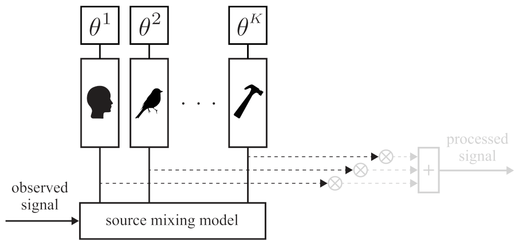
2.1. Problem Statement and Proposed Solution Framework

The goal of this work is to present an automated design methodology for monaural (single microphone-based) situated soundscaping algorithms for and by hearing aid users. With this methodology noise reduction algorithms can be tailored to an individual without the need of an intervening team of engineers. Our approach automates the design process by specifying the underlying signal processing algorithm design tasks as automatable inference tasks on a generative model. Because we do not have any specific information about observed signals in situated settings, we choose for a general modeling approach in which we assume that the received signal comprises a mixture of desired and undesired signals. These constituent source signals are modeled on the spot during the source modeling stage. For this purpose we use probabilistic sub-models that can be designed for stationary or non-stationary acoustic signals. These estimated sub-models are subsequently used in the source separation stage to extract the underlying source signals, which are then individually amplified or suppressed during the soundscaping stage according to the preferences of the user. In this section, we first introduce a minimal generative model for the observed mixture signal. Then, each task in the soundscaping framework (source modeling, source separation and soundscaping) is formally described as an automatable probabilistic inference procedure on this minimal generative model.
Consider an observed mixture signal x n at time steps n = 1 , 2 , , N , which is composed of latent source signals s n k , with k = 1 , 2 , , K denoting the source index. These latent source signals are modeled by latent states z n k , which are controlled by the time-invariant model parameters θ k . The generated output signal of the soundscaping system y n is a mixture of re-weighted source signals, controlled by user preferences w k , which we assume to be static in this work. Specifically, we define a generative model p ( y , w , x , s , z , θ ) , where the variables with omitted indices refer to the sets of those variables over the omitted variables, e.g., y = { y n } n = 1 N and s = { s k } k = 1 K , as
p ( y , w , x , s , z , θ ) = p ( w ) p ( θ ) p ( z 0 ) priors n = 1 N p ( y n w , s n ) soundscaping p ( x n s n ) source mixing k = 1 K p ( s n k , z n k z n 1 k , θ k ) source modeling .
Equation (1) factorizes the full generative model into three main factors: soundscaping p ( y n w , s n ) , source mixing p ( x n s n ) and source modeling p ( s n k , z n k z n 1 k , θ k ) . In this particular model, the K constituent source signals are assumed to be statistically independent. The source mixing term p ( x n s n ) describes how the observed signal x n is formed by its constituent source signals s n . The soundscaping factor p ( y n w , s n ) models the processed output signal y n based on the user preferences w k and individual source signals s n k . For modeling the source signals s n k we use the source modeling factor p ( s n k , z n k z n 1 k , θ k ) . This term describes how the source signal s n k and its latent state z n are modeled as a dynamical system with previous latent state z n 1 k and transition parameters θ k . Note that the source modeling term p ( s n k , z n k z n 1 k , θ k ) can be expanded or constrained according to the complexity of the signal that we wish to model. A further specification of the generative model will be given in Section 2.2. The resulting high degree of factorization in this model is a feature that we will take advantage of when executing inference through message passing in a factor graph.
Next, we will further specify our soundscaping framework using the example from the introduction, where background chatter disrupts a conversation. The inference tasks will be derived from (1) using a Bayesian approach by applying Bayes’ rule and by marginalizing over the nuisance variables.

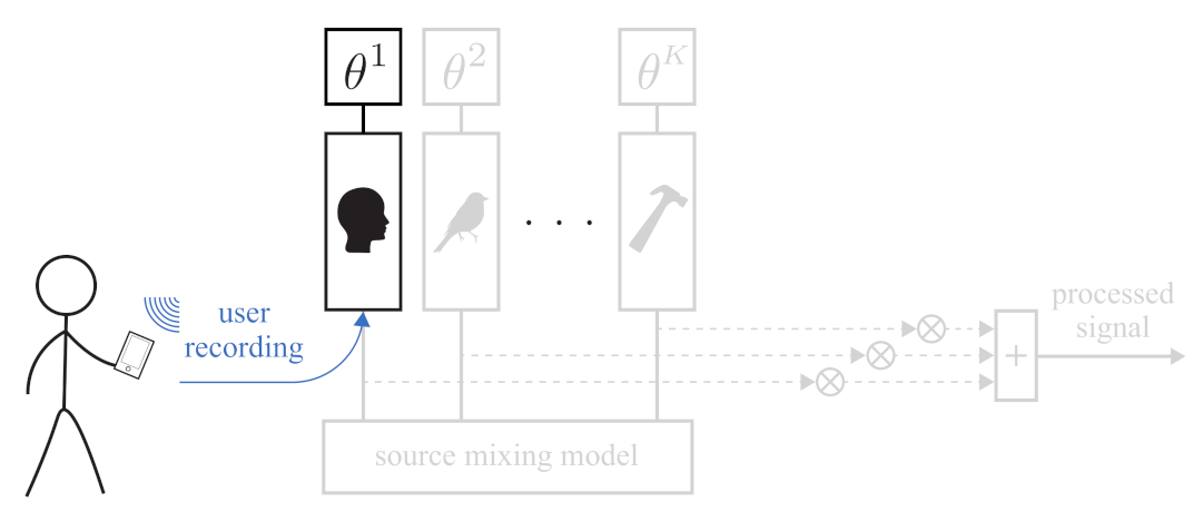
2.1.1. Source Modeling

In the first stage of the soundscaping framework, the source modeling stage, we need to infer model parameters for the constituent sources in the observed mixture. These constituent sources comprise the background chatter and the speech signal in the conversation. Before the source modeling stage can commence, the user has to record a fragment of both sounds individually. Both speech and chatter fragments are required to last approximately three seconds. This is short enough to impose little burden on the end user, while long enough to obtain relevant information about the acoustic signal. Alternatively, models for common complex acoustic signals, such as speech, can be estimated beforehand on some data sets. In this way, only a fragment of the noise has to be recorded, easing the burden on the user. For each source signal, the model parameters are then estimated through probabilistic inference, based on the recorded fragment. Figure 1 gives an overview of the source modeling stage.
Nowadays, commercial hearing aids (and other audio devices, such as headphones) come with an accompanying smartphone app to control the settings of the device. From a user experience perspective, we envision that the user has access to a user-friendly app on their mobile device. Here the user can intuitively record sounds for the individual sound models and can enable pretrained models for common sounds like speech through sliders and switches in the app. For creating these recordings, the users can use their mobile phone or a directional microphone for an improved selectivity.
The inference task corresponding to the source modeling stage for a single source involves calculating the posterior probability of the parameters θ k given a recorded fragment s ^ k as input. The source modeling task on the generative model (1) is therefore given by
p ( θ k s ^ k ) p ( θ k ) p ( z 0 k ) n = 1 N p ( s n k = s ^ n k , z n k z n 1 k , θ k ) d z k .
This expression is obtained by applying Bayes’ theorem and by marginalizing over the distributions of all nuisance variables. We assume that s ^ k is directly and solely observed, resulting in the simplified source mixing model corresponding to p ( x n | s n ) = δ ( x n s n ) , where δ ( · ) denotes the Dirac delta function. Note that (2) is in principle computable since the individual factors ( p ( θ k ) , p ( z 0 k ) and p ( s n k , z n k z n 1 k , θ k ) ) are readily specified in the generative model (1). The calculation of this equation can be performed using message passing as will be discussed in Section 2.3. The posterior probability of the parameters θ k from the first stage is consecutively used as the prior distribution of the parameters p ( θ k ) during the second stage as p ( θ k s ^ k ) .

2.1.2. Source Separation
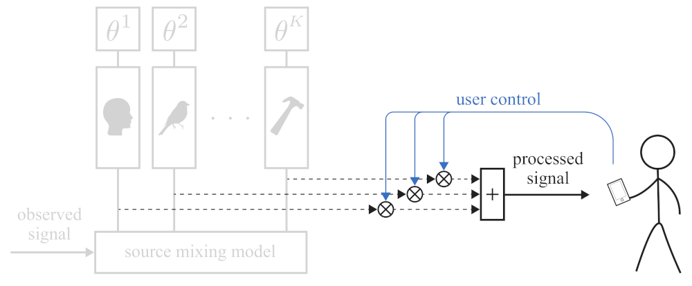
Stage two, the source separation task, concerns inverting the (generative) sound mixing model in (1), meaning that we are interested in recovering the constituent source signals s n 1 : K from a received mixture signal x 1 : n . Using the inferred source models from the first stage the constituent sources are separated from the mixture. This procedure is sometimes called “informed source separation” in the literature [6]. This approach contrasts to blind source separation methods where very little prior information about the underlying sources is available. In the proposed framework, informed source separation is performed through probabilistic inference for p ( s n x 1 : n , s ^ ) on the specified generative model, see Figure 2 for a graphical overview. Source separation by inference can then be worked out to
p ( s n x 1 : n , s ^ ) p ( z 0 ) i = 1 n p ( x i s i ) k = 1 K p ( s i k , z i k z i 1 k , s ^ k ) d s 1 : n 1 d z 0 : n ,
where
p ( s i k , z i k z i 1 k , s ^ k ) = p ( θ k s ^ k ) p ( s i k , z i k z i 1 k , θ k ) d θ k .
Again, note that all factors in (3) and (4) are already specified as factors in the generative model (1) or a result from the source modeling task of (2). Therefore, (3) and (4) are computable. Technically, (3) is a Bayesian filtering (state estimation) task that can be efficiently realized by (generalized) Kalman filtering [31,32]. We will automate this Kalman filtering task through message passing in a factor graph representation of the generative model.

2.1.3. Soundscaping

Finally, in the (third) soundscaping stage, the estimated source signals form the basis of the new acoustic environment of the user. By user-driven re-weighing of these source signals, desired signals can be enhanced and undesired signals can be suppressed. This re-weighing operation seeks a perceptually pleasing balance between residual noise and speech distortion that result from the source separation stage. From a user experience perspective, we envision that the user has access to additional sliders in the smartphone app to tune the gain for each source signal in the enhanced mixture produced by the hearing aid, as shown in Figure 3. The soundscaping stage can be cast as the following inference task:
p ( y n x 1 : n , s ^ ) p ( w ) p ( y n w , s n ) p ( s n x 1 : n , s ^ ) d w d s n .
On the right-hand side (RHS) of this equation, the factor p ( s n x 1 : n , s ^ ) is available as output of the source separation stage. The other RHS factors, the prior on the user preferences p ( w ) and the function that generates the re-weighted signal p ( y n w , s n ) , have already been specified by creating the full generative model (1). Therefore, soundscaping by inference as specified by (5) is computable.
In summary, in this section we have outlined a probabilistic modeling-based framework for situated soundscaping design. Crucially, all design tasks, namely (2) for source modeling, (3) for source separation and (5) for soundscaping, have been phrased as automatable inference tasks on a generative model (1). For the application of this framework to real-world problems we first need to further specify the generative model of (1) (Section 2.2). Next we need to describe how the above inference tasks are realized (Section 2.3). After these steps, the soundscaping framework under the chosen model specification can be applied and can be validated using experiments (Section 3).

2.2. Model Specification

In this section we apply our framework on two example generative probabilistic models for mixtures of acoustic signals as a further specification of the minimal generative model in (1). The two example models consist of two distinct source mixing models and similar submodels for the constituent signals. First, we introduce the source mixing models, based on the Algonquin algorithm [9] and Gaussian scale models [30], respectively. In other words, we provide explicit specifications for the source mixing model p ( x n s n ) in (1). Next, we use the Gaussian mixture model (GMM) as the source model p ( s n k , z n k z n 1 k , θ k ) in (1).

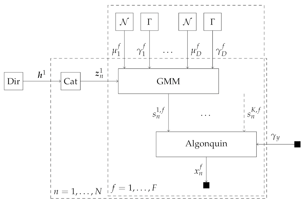
2.2.1. Source Mixing Model 1: Algonquin Model

The Algonquin-based source mixing model acts on the log-power coefficients of an acoustic signal. Therefore, first the complex frequency coefficients are obtained from windowed signal frames of length F of the observed temporal acoustic signal. These coefficients can be computed using the short-time Fourier Transform (STFT), but in our application we will make use of a frequency-warped filter as we will describe thoroughly in Section 3.3. Let X n = X n 1 , X n 2 , , X n F denote the vector of observed independent and identically distributed (IID) complex frequency coefficients, where X n f C for every frame n = 1 , 2 , , N and every frequency bin f = 1 , 2 , , F . We assume our observed acoustic signal to be a sum of K constituent signals. Owing to the linearity of the STFT, X n can therefore be expressed as
X n = k = 1 K S n k ,
where S n k = S n k , 1 , S n k , 2 , , S n k , F represents the vector of complex frequency coefficients corresponding to the n th frame of the k th constituent signal.
The Algonquin algorithm [9] performs source separation on the log-power spectrum. It approximates the observed log-power spectrum coefficients x n f = ln ( | X n f | 2 ) , using the log-power spectrum coefficients of the constituent signals s n k , f = ln ( | S n k , f | 2 ) , as
x n f = ln k = 1 K exp s n k , f + k j exp s n k , f + s n j , f 2 cos θ n k , f θ n j , f ln k = 1 K exp s n k , f ,
where θ n k , f represents the phase corresponding to the f th frequency bin of the n th frame of the k th constituent signal. The phase information is neglected as the resulting source mixing model, assuming uniform and independent phases, leads to intractable inference [10]. This neglected phase interaction is post hoc accounted for by modeling it as Gaussian noise, leading to the Algonquin source mixing model
p a x n f s n 1 , f , , s n K , f = N x n f | ln k = 1 K exp s n k , f , γ x 1 ,
where the tuning parameter γ x represents the precision of the Gaussian distribution to account for the neglected phase interaction between the different constituent signals in (7).

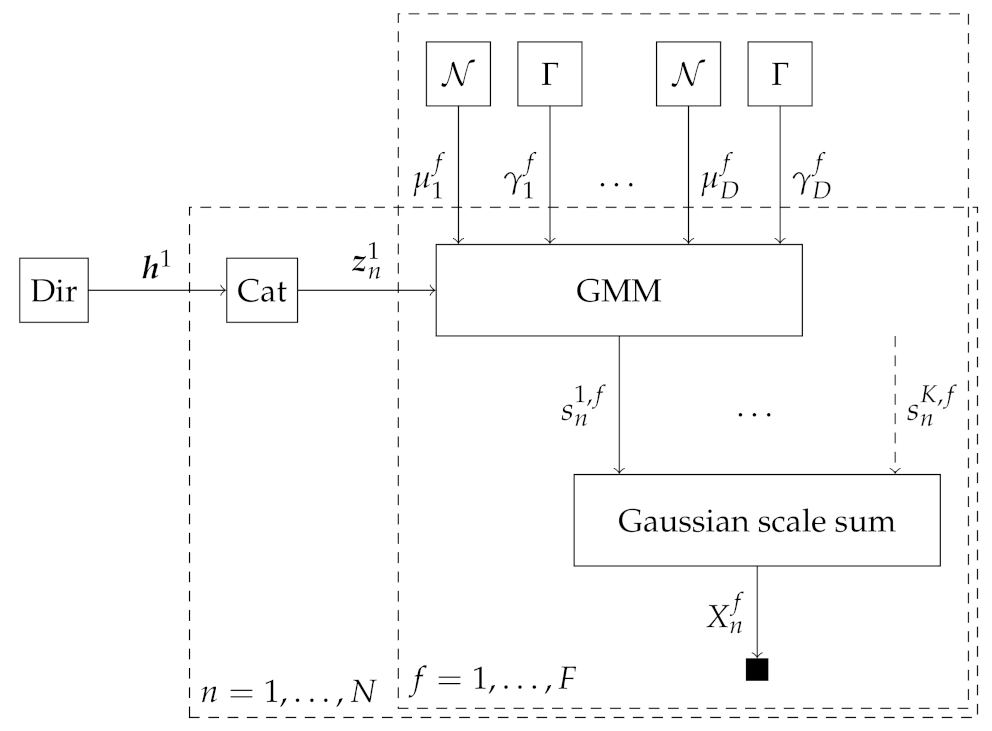
2.2.2. Source Mixing Model 2: Gaussian Scale Sum Model

The Algonquin model requires estimation of the noise variance γ x 1 . Here we present an alternative novel source mixing model that does not require any tuning parameters, inspired by the Gaussian scale models from [30].
We assume a (complex) Gaussian distribution for the frequency coefficients of the constituent signals S n k , given by
S n k N C μ , Γ , C ,
with mean μ = 0 , complex covariance matrix Γ and relation matrix C, see [33] for more details. In order to keep inference tractable, independence is assumed between the real and imaginary parts of the coefficients, requiring C = 0 . Following [30], the covariance matrix Γ is modelled as a diagonal matrix with exponentiated auxiliary variables s n k , f , leading to the model
p ( S n k , f s n k , f ) = N C S n k , f 0 , exp s n k , f , 0 = exp s n k , f π exp exp s n k , f | S n k , f | 2 .
This probabilistic relationship shows great similarity with the transform from the frequency coefficients to the log-power spectrum, as its log-likelihood can be found as ln p ( S n k , f s n k , f ) = s n k , f exp ( s n k , f ) | S n k , f | 2 ln ( π ) and from this description the maximum of s n k , f can be found to occur at s n k , f = ln ( | S n k , f | 2 ) , which coincides with the deterministic transform from the frequency coefficients to the log-power spectrum. As a result of this observation, the variables s n k = s n k , 1 , , s n k , F are in this model termed the pseudo log-power coefficients of the original source signal S n k . Due to the linearity of the STFT in (6), the likelihood function of X n f can be expressed using (10) as
p g X n f s n 1 , f , , s n K , f = N C X n f | 0 , k = 1 K exp s n k , f , 0 .
In contrast to the Algonquin model, this Gaussian scale sum model does not contain any tuning parameters and operates on the complex frequency coefficients instead of the log-power spectrum. Note that the pseudo log-power coefficients s n k , f are not exactly equal to the deterministic log-power coefficients of the Algonquin-based source mixing model, although they show great similarity.
As we have defined the observed signal as a function of the constituent signals, the next task concerns modeling the constituent signals s n k = [ s n k , 1 , , s n k , F ] themselves. In this paper, we will use a Gaussian mixture model for this purpose.

2.2.3. Source Model: Gaussian Mixture Model

In this paper we use a Gaussian mixture model as a prior for the (pseudo) log-power coefficients s n as
p ( s n μ , γ , z n ) = d = 1 D f = 1 F N s n f μ d f , ( γ d f ) 1 z n d ,
where the source index k is omitted for compactness of notation. Here we assume independence between the frequency bins to ease computations ([34], pp. 64–65). The mixture components are denoted by d = 1 , 2 , , D . The mixture means μ = [ μ 1 , , μ D ] are modeled as
p ( μ d ) = f = 1 F N μ d f m d f , v d f ,
where μ d = [ μ d 1 , , μ d F ] and where m d f and v d f represent the mean and variance of the mixture mean μ d f , respectively. Similarly the mixture precisions γ d = [ γ d 1 , , γ d F ] are modelled as
p ( γ d ) = f = 1 F Γ ( γ d f a d f , b d f ) ,
where Γ ( · α , β ) denotes the Gamma distribution with shape and rate parameters α and β , respectively. a d f and b d f represent the shape and rate parameters of the mixture precision γ d f , respectively.
We use one-hot encoding [28] to represent mixture selection variables z n = [ z n 1 , , z n D ] , thus d = 1 D z n d = 1 and z n d { 0 , 1 } . We assume a categorical prior distribution for z n
p ( z n h ) = Cat ( z n h , D ) ,
where D denotes a number of components and h the event probabilities. Finally, we model h using a Dirichlet prior as
p ( h ) = Dir ( h α ) ,
where α = [ α 1 , , α D ] are the concentration parameters.
In summary, in this section we have further specified the generative model of (1). To apply the proposed framework, two distinct models have been specified. The first model is based on the Algonquin-based source mixing model, in which the individual signals are represented by Gaussian mixture models. This first probabilistic model is fully specified by (8), (12)–(16). Secondly, an alternative model has been presented, which is based on Gaussian scale models. This probabilistic model is fully specified by (11)–(16). The soundscaping framework supports different acoustic models, concerning both the source mixing models as the source models.

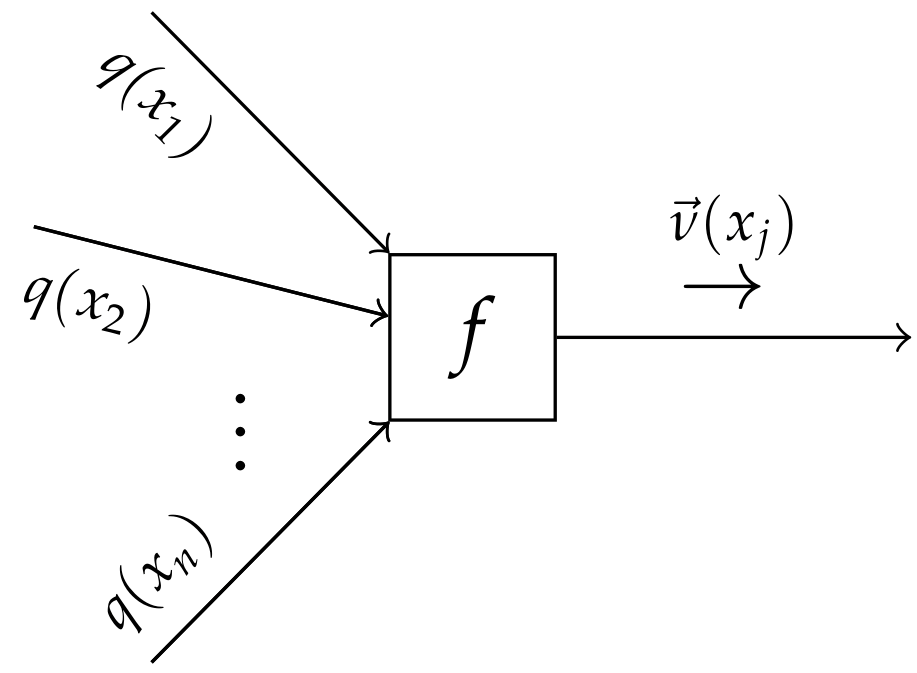
2.3. Factor Graphs and Message Passing-Based Inference

As described in Section 2.1, the source modeling, source separation and soundscaping tasks can be framed respectively as inference tasks for computing p ( θ k s ^ k ) , p ( s n x 1 : n , s ^ ) and p ( y n x 1 : n , s ^ ) on the generative model. Before describing how inference is realized in our generative model, we present a brief review of factor graphs and message passing algorithms. We use message passing in a factor graph as our probabilistic inference approach of choice, due to of its efficiency, automatability, scalability and modularity [25,32]. Factor graphs allow us both to visualize factorized probabilistic models as graphs and to execute inference by automatable message passing algorithms on these graphs.

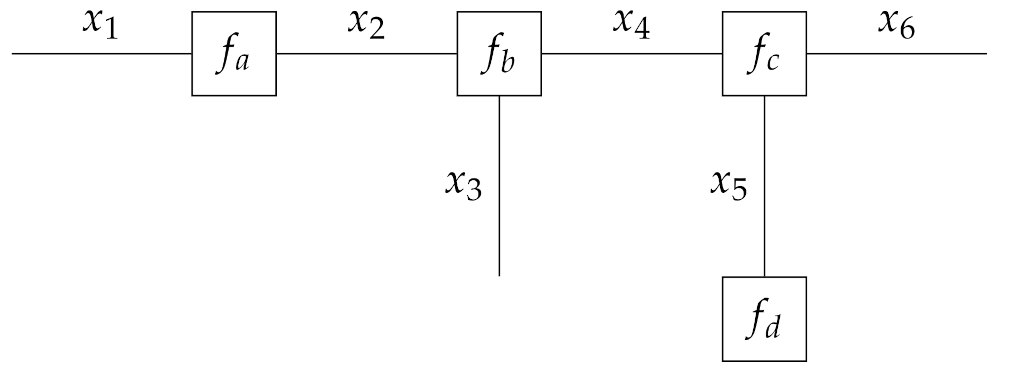
2.3.1. Forney-Style Factor Graphs

Factor graphs are a class of probabilistic graphical models. We focus on Forney-style factor graphs (FFG), introduced in [35], with notational conventions adopted from [36]. The interested reader may refer to [32,36] for additional information on FFGs. FFGs visualize global factorizable functions as an undirected graph of nodes corresponding to the local functions, or factors, connected by edges or half-edges representing their mutual arguments. This factorized representation allows naturally for the visualization of conditional dependencies in generative probabilistic models.
Here we will represent the factorizable probability density function p ( x 1 , x 2 , x 3 , x 4 , x 5 , x 6 ) using an FFG. Assume this function factorizes as
p ( x 1 , x 2 , x 3 , x 4 , x 5 , x 6 ) = f a ( x 1 , x 2 ) f b ( x 2 , x 3 , x 4 ) f c ( x 4 , x 5 , x 6 ) f d ( x 5 ) ,
where the functions with alphabetical subscript denote the individual factors. The FFG, as shown in Figure 4, can be constructed from (17) following the three visualisation rules of [36].
One of the most apparent constraints of these graphs specifying that edges can be connected to a maximum of two nodes, can easily be circumvented through the use of a so-called equality node and the introduction of two variable copies. Suppose a variable y is the argument of three factors. The introduction of an equality node function f = ( y , y , y ) = δ ( y y ) δ ( y y ) , where δ ( · ) represents the Dirac delta function, allows for branching y into variable copies y and y . The equality node constrains the beliefs over y, y and y to be equal.
Figure 5 shows a (Forney-style) factor graph representation of the proposed generative Algonquin-based model. This representation simplifies the model as outlined by (8), (12)–(16). Furthermore Figure 6 shows the FFG of the Gaussian scale sum-based generative model, specified by (11)–(16). In these figures a single source model (the Gaussian mixture model) has been drawn to prevent clutter.

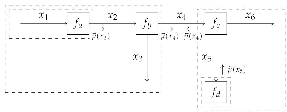
2.3.2. Sum-Product Message Passing

Suppose that we would like to calculate the marginal distribution p ( x 4 ) , which is the probability distribution of x 4 obtained by marginalizing over the distributions of all other random variables in (17). Here we implicitly assume that all random variables are continuous and therefore marginalization is performed through integration instead of summation. If p ( x 1 , x 2 , x 3 , x 4 , x 5 , x 6 ) were not factorizable, the marginal could be calculated as
p ( x 4 ) = ... p ( x 1 , x 2 , x 3 , x 4 , x 5 , x 6 ) d x 4 ,
where x j denotes the set of all variables x i i excluding x j . However, the conditional independencies amongst some of the variables allow for the use of the distributive property of integration in rewriting (17) as
p ( x 4 ) = f a ( x 1 , x 2 ) d x 1 μ ( x 2 ) f b ( x 2 , x 3 , x 4 ) d x 2 d x 3 μ ( x 4 ) · f a ( x 1 , x 2 ) d x 1 μ ( x 2 ) f b ( x 2 , x 3 , x 4 ) d x 2 d x 3 f c ( x 4 , x 5 , x 6 ) f d ( x 5 ) μ ( x 5 ) d x 5 d x 6 μ ( x 4 ) .
Here the global computation of (18) is executed through a set of local computations, denoted by μ , which can be interpreted as messages that nodes in the graph send to each other. These messages are visualized in Figure 7 and can be thought of as a summaries of inference in the corresponding dashed boxes. The FFG now has arbitrarily directed edges to indicate the flow of the messages. A message μ ( x ) propagating on edge x is denoted by μ ( x ) or μ ( x ) when propagating in or against the direction of the edge, respectively.
The message μ ( x j ) flowing out of an arbitrary node f ( x 1 , x 2 , , x n ) with incoming messages μ ( x j ) is given by
μ ( x j ) f ( x 1 , x 2 , , x n ) i { 1 , , n } j μ ( x i ) d x j
which is called the sum-product update rule [38]. This update rule is the core of the sum-product message passing algorithm, which is also known as belief propagation. This algorithm concerns the distributed calculations of various marginal functions from a factorizable global function. In the previous example the FFG was acyclic and therefore a finite predetermined number of messages is required for convergence. If this graph would have included cycles, an iterative message passing schedule would be required. This is known as loopy-belief propagation and its convergence is not guaranteed [39].

2.3.3. Variational Message Passing

In some instances, the integrals in the sum-product update rule (20) can become intractable. Linear Gaussian models are an example of a class of models in which sum-product messages can be calculated in closed-form expressions. However, in models such as the Algonquin model of (8) the integrals become intractable. In these cases, we can resort to an approximate message passing algorithm, called variational message passing (VMP) [40,41], which gives closed-form expressions for conjugate pairs of distributions from the exponential family. If closed-form expressions with VMP are still not available, we might resort to approximation methods, such as importance sampling or Laplace’s method [42].
Suppose that we are dealing with a generative model p ( y , z ) with an intractable posterior distribution p ( z y ) , where y and z denote the observed and latent variables, respectively. The goal of variational inference is to approximate the intractable true posterior with a tractable variational distribution q ( z ) through minimization of a variational free energy functional
F [ q ] = D KL [ q ( z ) | | p ( z y ) ] ln p ( y ) .
where D KL is the Kullback-Leibler divergence and which is, in the machine learning literature, also known as the negative Evidence Lower BOund (ELBO) [43] as it bounds the negative log-evidence ln p ( y ) , because D KL 0 for any choice of q. Since the second term of (21) is independent of q ( z ) , free energy minimization is equivalent to the minimization of the Kullback-Leibler divergence. Furthermore, the variational free energy can be used as an approximation to the negative log-evidence for techniques such as Bayesian model selection, Bayesian model averaging [44] and Bayesian model combination [45].
In practice, the optimization of (21) is performed by imposing additional constraints on q ( z ) , e.g., by limiting q ( z ) to a family of distributions, or by additional factorization assumptions (e.g., q ( z ) = i q i ( z i ) which is known as the mean-field assumption). Depending on the constraints on q ( z ) , the minimization of (21) can be achieved through sum-product message passing or variants of VMP. In the latter case, the goal is to iteratively update the variational distributions through coordinate descent on (21). In general, the variational message ν ( x j ) from a generic node f ( x 1 , x 2 , , x n ) with incoming marginals q ( x j ) (see Figure 8) can be written as [41]
ν ( x j ) exp i { 1 , , n } j q ( x i ) ln f ( x 1 , x 2 , , x n ) d x j .
Given these messages, the variational distributions can be updated through the multiplication of the forward and backward message on that respective edge as
q ( x j ) ν ( x j ) ν ( x j ) .

2.3.4. Automating Inference and Variational Free Energy Evaluation

For frequently-used elementary factor nodes, the message update rules (20) and (22) can be derived analytically and saved in a lookup table. Message passing-based inference then resorts mainly to substituting the current argument values in worked-out update rules. A few open source toolboxes exist for supporting this type of “automated” message passing-based inference. In this paper, we selected ReactiveMP (ReactiveMP is available at https://github.com/biaslab/ReactiveMP.jl, accessed on 1 July 2021), the successor of ForneyLab (ForneyLab is available at https://github.com/biaslab/ForneyLab.jl, accessed on 1 July 2021) [25], to realize the previously described inference tasks (2), (3) and (5). ReactiveMP is an open source Julia package for message passing-based inference that specifically aims to excel at real-time inference in dynamic models. This package allows us to specify a generative model and to perform automated inference on this model. The desired distributions of (2), (3) and (5) are therefore automatically calculated. Furthermore, ReactiveMP automatically evaluates the performance of the model on the data by calculating the Bethe free energy [46], which equals the variational free energy for acyclic graphs. This free energy is calculated using node-local free energies and the edge-local entropies of the random variables, where we can also impose local constraints on these variables for a trade-off between tractability and accuracy of the free energy calculation [47].
In this paper we have introduced the Algonquin model in (8) and the Gaussian scale sum model in (11). Inference in these models is non-trivial and therefore in the next two subsections we will describe how to perform message passing-based inference in these models, such that we can automate message passing in the proposed generative models of Section 2.2. Furthermore we derive the node-local free energies for the automated evaluation of model performance using the variational free energy.

2.3.5. Message Passing-Based Inference in the Algonquin Model

Exact inference in the Algonquin model of (8) leads to intractable inference, because the non-linear relationship leads to non-Gaussian distributions [9]. Approximate inference by variational message passing also results in difficulties. For the variational messages the expectation has to be determined over the mean term of (8). The expectation over this so-called log-sum-exp relationship has, however, no analytical solution and needs to be approximated as in [9,48,49]. Ref. [50] gives an overview of the available approximations methods. In this paper we will comply with the original approximation from [9]:
ln k = 1 K exp ( s k ) ln k = 1 K exp ( s k ) | s k = E s k + s ln k = 1 K exp ( s k ) | s k = E s k s E s ,
where the notation of (8) is altered to prevent clutter. The subscript (and former superscript) k now denotes the source index and the frame and frequency bin indices are omitted. With this approximation, the mean of (8) is approximated using a first-order vector Taylor expansion. The function is linearly expanded around the mean of the constituent signals s k .
Table 1 gives an overview of the Algonquin node of (8). This node has been generalized with respect to [9] to accommodate for more than 2 sources and to also allow for inferring the noise precision γ x . The table shows the variational messages under the mean-field assumption and using the vector Taylor expansion. Finally, the local variational free energy is presented in the table. All derivations can be found at our GitHub repository (the GitHub repository can be accessed at https://github.com/biaslab/SituatedSoundscaping, accessed on 1 July 2021). Of particular interest are the messages ν ( s k ) in Table 1, because their parameters carry an interesting interpretation. First it is important to note that the messages ν ( s k ) depend on the mean E q ( s k ) s k . This is a result of the expansion point of the Taylor expansion. Thus, the message ν ( s k ) gets calculated according to the current mean over the edge of s k , that mean gets updated according to the incoming message and this procedure iteratively repeats. Furthermore, attention should be paid to the variances of the messages ν ( s k ) . These are normalized using a softmax function over the constituent sources, which means that only the most dominant sources receive informative messages. The messages towards the less-dominant sources all have relatively high variances and will not significantly alter the posterior distributions. This is desired as the information from our observations will mostly update the most dominant sources, which have the biggest impact on the observation.

2.3.6. Message Passing-Based Inference in the Gaussian Scale Sum Model

Similarly to the Algonquin node, exact inference is also not possible in the Gaussian scale sum node of (11). Also variational message passing yields intractable computations. As a result we again need to perform a vector Taylor expansion for approximating the intractable terms, corresponding to the covariance term in (11). Table 2 shows an overview of the Gaussian scale sum node, the corresponding variational messages and the node-local variational free energy. All derivations can be found at our GitHub repository (the GitHub repository can be accessed at https://github.com/biaslab/SituatedSoundscaping, accessed on 1 July 2021).
The message ν ( s k ) has been calculated by approximating the intractable terms using a vector Taylor expansion over all variables, except for s k . Alternative approaches are also feasible. For example, approximating the intractable terms using a full vector Taylor expansion (also over s k ), as with the Algonquin node, is also feasible, although this would result in an improper variational log-message that is linear in s k . As can be seen in Table 2, the variational message ν ( s k ) does not belong to a well-known probability distribution. As the sigmoidal shape of ν ( s k ) prevents us from directly approximating this variational message by a common distribution, we propagate the message ν ( s k ) in its functional form, calculate the marginal and then approximate the marginal by a well-known distribution for tractability. Therefore we pass the functional form as a message over the graph. We then derive a functional form of the resulting marginals and approximate the marginals with a Gaussian distribution for tractability. Here the log-marginal ln q ( s k ) is approximated by a second-order Taylor expansion at its mode as
ln q ( s k ) ln q ( s k , 0 ) + 1 2 d 2 ln q ( s k ) d s k 2 | s k = s k , 0 ( s k s k , 0 ) 2
where s k , 0 is the mode of the marginal. Because the message is expanded around its mode, the first-order derivative vanishes from the Taylor expansion. This mode can be found by solving d ln q ( s k ) d s k = 0 for s k . In our case there is no closed-form solution for the mode and therefore we need to resort to numerical optimization for finding this maximum.

2.3.7. Implementation Details

Now that the probabilistic models have been defined in Section 2.2, the three inference tasks from Section 2.1 remain: source modeling (2), source separation (3) and soundscaping (5). For better initialization of the source models and for proper unbiased source separation using mixture models, several additional steps have been taken to implement the described inference procedures. The interested reader may refer to Appendix A for a detailed specification of the inference procedures from Section 2.1.

3. Experimental Validation

Now that we described the situated soundscaping framework and presented relevant generative models, we evaluate the framework on a simulated real-life scenario. Here a speech signal is corrupted by background noise. This section first describes the experimental setup, data selection and preprocessing procedures. Then we describe the performance metrics that we use to evaluate our framework under the different models from Section 2.2. Finally, we present and discuss the results obtained for the current models.

3.1. Experimental Overview

Two different experiments were conducted in this research to validate our proposed framework for the models from Section 2.2. In both experiments, the source model for the speech signal was pretrained offline, as speech signals are inherently complex to model and a short fragment will not be enough to capture all characteristics of speech. The noise model is trained on three seconds of the noise signal, which should be recorded in-the-field by the user. During the source separation stage in both experiments 10 s of the mixture signal, consisting of a speech and noise signal, is processed. In both experiments the signal-to-noise ratio (SNR) of the input signal is varied for a constant number of mixture components for the speech and noise model. The number of mixture components of the speech model has been set to 25. In the first and second experiment the number of noise clusters is set to 1 and 2, respectively.

3.2. Data Selection

Two data sets have been used for experimental validation:
  • The LibriSpeech data set (the LibriSpeech data set is available at https://www.openslr.org/12, accessed on 31 March 2021) [51], which is a corpus of approximately 1000 h of 16 kHz read English speech.
  • The FSDnoisy18k data set (the FSDnoisy18k data set is available at https://www.eduardofonseca.net/FSDnoisy18k, accessed on 13 April 2021) [52], is an audio data set, which has been collected with the aim of fostering the investigation of label noise in sound event classification. It contains 42.5 h of audio samples across 20 sound classes, including a small amount of manually-labeled data and a larger quantity of real-world noise data.
From the LibriSpeech data set the first 1000 audio excerpts, consisting of approximately 200 min of speech, are used to train the speech source model. Besides this a random speech excerpt has been selected, outside of the first 1000 excerpts, to perform source separation and soundscaping. From the FSDnoisy18k data set also a random noise excerpt has been selected, in this case representing a clapping audience. The first 3 s of this signal were used to train the noise model and the consecutive 10 s were used for source separation and soundscaping.

3.3. Preprocessing

All signals were first resampled to 16 kHz, since most of the speech intelligibility information is located below 7 kHz. Furthermore the computational load increases sharply for higher sampling frequencies, which is incompatible with the ultra-low power demands of hearing aids. After resampling the speech and noise signals are centered around 0. The speech signal is power-normalized to 0 dB and the noise signal is power-normalized to obtain the desired SNR for the experiments.
Next, the signal is processed by a frequency-warped filter for two reasons, for detailed discussions see [53]. First, we would like to obtain a high frequency resolution for source separation to be more efficient. Extracting the frequency coefficients directly using the short-time Fourier transform would require processing longer blocks of data for obtaining a higher frequency resolution. This leads to the second reason: we would like to limit the processing delay of the hearing aid. A large processing delay leads to coloration effects when the hearing-aid user is talking, which is experienced as “disturbing” by the user [53]. From this it becomes evident that we need to compromise between both goals when directly using the STFT. The frequency-warped filter achieves both goals by warping the linear frequency scale to a perceptually more accurate frequency scale, also known as the Bark scale [54]. For the same block size it achieves a perceptually higher frequency resolution in comparison to the STFT.
The frequency-warped filter consists of a series of first-order all-pass filters. The Z-transform for a single all-pass filter is given by
A ( z ) = z 1 a 1 a z 1 ,
with warping parameter a. At a sampling frequency of 16 kHz, the warped frequency spectrum best approximates the Bark scale for a = 0.5756 [55]. The frequency-warped spectrum can be obtained by calculating the fast Fourier transform (FFT) over the outputs of each all-pass section, often referred to as taps. Because of conjugate symmetry in the obtained frequency coefficients, about half of the coefficients is discarded to limit computational complexity. From the remaining coefficients the input of the source modeling stage is formed. Importantly, the frequency-warped filter will also be used for reconstructing the signal by adding an FIR compression filter to it, as done in [53]. Here the “Gain calculation” block in ([53], Figure 3) will encompass the source separation and soundscaping stages in our framework. Throughout all experiments we will use a frequency-warped filter of length F = 32 , which yields 17 distinct frequency coefficients, with a step size of 32 for reduced computations.

3.4. Performance Evaluation
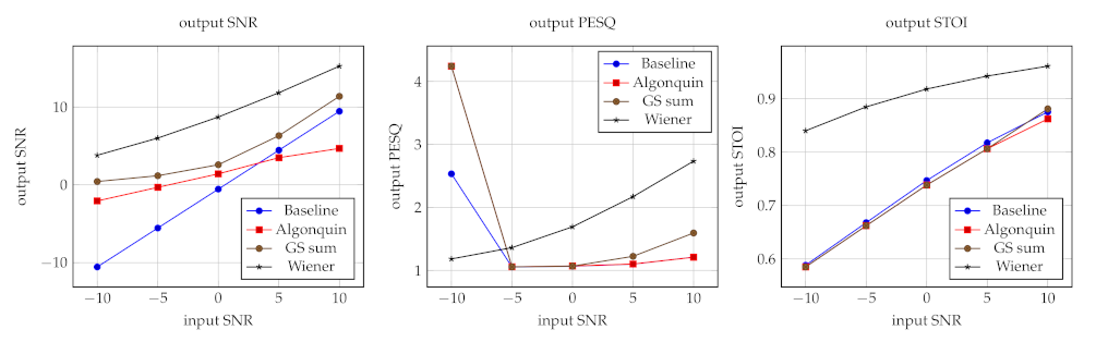
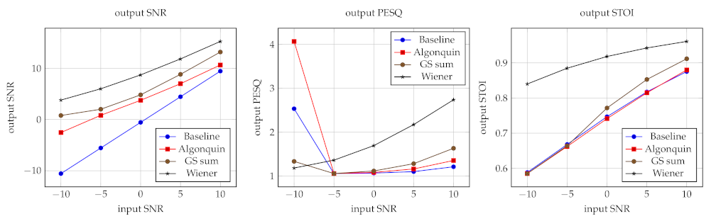
Our presented novel methodology differs from conventional research in the fact that users can create their personalized soundscaping algorithms by performing automated probabilistic inference on a modular generative model, with interchangeable submodels trained using on-the-spot recorded sound fragments. Users can adjust the source-specific gains w for balancing the amount of noise reduction and the inevitable introduction of speech distortion. Throughout the experiments the parameter w is post-hoc optimized subject to w k [ 0 , 1 ] and k w k = 1 to yield the most optimal performance metric, as in a real setting we assume that the user is capable of setting these parameters to their most optimal value. For comparison we will also evaluate the performance of the noise corrupted situation before and after processing with a Wiener filter [56].
A Wiener filter assumes full knowledge about the underlying signals and was implemented as follows. The mixture signal and the underlying signals are all processed by separate frequency-warped filters Every segment of data, consisting of 32 samples, is fed into the frequency warped filter. The frequency coefficients are extracted using the STFT and based on those the signal powers are calculated for each frequency bin as their squared magnitudes. The Wiener filter gain for each of the frequency bins is calculated individually as G f = P s f / ( P s f + P s f ) , where G f is the Wiener filter gain for frequency bin f and where P s f and P s f represent the corresponding calculated powers of the speech signal and noise signal, respectively. This gain is applied to the FIR compression filter to determine the processed output signal.
Finally, a quantitative measure for assessing the performance is not straightforward, because the performance depends on the perception of a specific individual human listener, and there are no personalized metrics for this application. In order to evaluate our approach we evaluate several metrics, of which some have been developed to approximate human perception. In this paper we evaluate the model performance using the output SNR, the perceptual evaluation of speech quality (PESQ) metric [57] and the short-time objective intelligibility measure (STOI) metric [58]. The output SNR represents the ratio of signal power with respect to noise power. It gives a quantitative impression of the remaining noise of the denoised signal by comparing it with the true signal. However, the output SNR does not measure the perceptual performance of the noise reduction algorithms. In contrast, the PESQ metric [57], introduced in 2001, is a more advanced metric that has been introduced to better model the perceptual performance. It was intended for a wider variety of network conditions and has been show to yield a significantly higher correlation with subjective opinions with respect to other perceptual evaluation metrics. The STOI metric [58], introduced in 2011, provides a measure for speech intelligibility that only uses short-time temporal speech segments, based on the correlation between the temporal envelopes of the extracted and true speech signal. It is important to note here that the PESQ and STOI metric represent by definition a group average of the experienced perceptual quality. The PESQ scores range from 1.0 (worst) to 4.5 (best) and the STOI scores range from 0.0 (worst) to 1.0 (best).

3.5. Results

The obtained results are visualized in Figure 9 and Figure 10. They show the model performance of the experiments from Section 3.1 with 1 and 2 noise mixture components, respectively.
In Figure 9 the output SNR, PESQ and STOI are calculated for a varying input SNR for both models of Section 2.2 with 1 noise mixture component. Besides the Wiener filter, the baseline performance, which corresponds to the output signal of the FIR compression filter for unity gain, is also plotted. The offset in the baseline output SNR with respect to the input SNR is caused by the frequency-warped filter. The input SNR is calculated with respect to the signals that enter the frequency-warped filter. After the processing by the filter the frequency-dependent phase delays lead to slightly degraded output SNRs, resulting in a vertical offset in the input and output SNR relationship.
The PESQ scores for an input SNR of −10 dB for the baseline and Algonquin model are incorrect as they by far outperform the Wiener filter for high noise situations. Therefore these points are regarded as outliers, possibly due to computational stability issues of the PESQ metric, as it was originally intended for narrowband telephone speech. From the figures it becomes evident that the Wiener filter yields the highest source separation performance in terms of output SNR, PESQ and STOI. This is expected as the Wiener filter requires full knowledge about the underlying signals in the observed mixture. In terms of PESQ scores, the Gaussian scale sum-based model attains better performance in comparison to the baseline signal.
In Figure 10 the output SNR, PESQ and STOI are calculated for a varying input SNR for both models of Section 2.2 with 2 noise mixture components, including the baseline performance and performance obtained with a Wiener filter. From all three plots it can be noted that the performance with respect to the baseline model has improved, especially for high input SNRs. In comparison to Figure 9, we can also see that the performance has increase when introducing an additional noise mixture model components. This behaviour is expected as we can model the source more accurately.

4. Discussion

From Figure 9 and Figure 10 it can be noted that the proposed soundscaping framework is capable of achieving increased speech quality for the current models. The performance metrics are inherently tied to the soundscaping weights w. Making adjustments to these weights can significantly increase the PESQ and STOI scores above the baseline performance. However, it should be noted that the PESQ and STOI metrics are by definition average group metrics. Therefore we expect that personalization of the weights w will lead to better perceived speech quality scores.
This paper lies at the foundation of a novel class of personalized and situated hearing aid algorithms. In the current framework the parameter estimation approach and the signal processing algorithm follow naturally from minimizing the variational free energy through probabilistic inference in a generative model. The framework allows hearing aid users to develop their own algorithms according to their preferences. Therefore it will ease the burden on hearing aid users as they do not need the help of specialists to personalize their hearing experience. This will greatly shorten the personalization procedure for users and is likely to yield more satisfying results. Although the main application of this paper concerned hearing aids, its generality extends to a broader class of applications. The framework is a thorough specification of the principle of informed source separation [6]. Therefore its usage extends to any source separation problem where information about the underlying sources is known or can be acquired, such as in denoising problems in biomedical signal processing or communication theory.
Future steps include the incorporation of user feedback and the learning of the acoustic model structure. Both improvements can be based on the same principle of free energy minimization, whose research fields are known as active inference [59] and Bayesian model reduction [60,61], respectively. The active inference approach to preference learning has the goal of imposing as little burden on the user as possible. We envision the user giving feedback to the algorithm through an accompanied app, which will be used for optimizing the source-specific gains depending on the acoustic context. Through Bayesian model reduction, the algorithm will automatically learn the optimal pruned model structure from a very generic probabilistic model by optimizing the free energy, which equals the simultaneous optimization of both the model accuracy and model complexity. This last step is required to bring down the computational complexity as the current implementation for the specified model is not yet suitable for real-time usage in hearing aid devices. This is a result of the inherent complexity of mixture models and the variational approximations which require multiple iterations for convergence. Instead, in future developments we may try to create sparse hierarchical time-varying source models that do not require variational approximations, such that the optimal result can be calculated within a single iteration. Furthermore, we can leverage the local stationarity in acoustic signals to only update the hearing aid gains (as described in Appendix A.3) every couple of milliseconds. By applying a combination of these approaches together with optimization of the framework we expect a real-time implementation of the framework to be within reach.
Besides the aforementioned directions for future research, we expect to obtain significant performance gains by altering the source model structure and by perhaps modeling the signal using an observation model in which inference is tractable and does not require variational approximations. In the current model proposals there are several straightforward directions for improving the separation performance. First, the Gaussian mixture models can both be extended using a Dirichlet process prior for determining an appropriate number of clusters. For computationally constrained devices, care should be taken with the number of clusters if real-time applications are desired. Bayesian model reduction [60,61] would prove itself useful here for pruning the number of clusters in an informed way, by monitoring the corresponding loss in variational free energy. Secondly, the Algonquin-based model can be optimized for all signals and SNRs. In the experiments we empirically set γ x = 10 , however, this is likely not to always yield optimal performance. By defining γ x as a random variable with a Gamma distribution prior, we could learn the optimal noise parameter. In Table 1 we have already derived novel variational messages for this purpose. Besides improving upon the current probabilistic models, we could also create entirely new probabilistic models for the underlying signals. Inspiration for these models can be obtained by reviewing architectural ideas of state-of-the-art deep neural networks. These large neural networks provide interesting ideas for further research on how to extend our compact generative model. For example, reference [20] uses dilated convolutions to mimic the hidden Markov dependencies among multiple samples. Reference [21] models the conventionally used Mel-spectrogram and models different types of spectro-temporal dependencies. Reference [22] extends the efficiency of neural networks by using conventional audio processing blocks, such as oscillators and synthesizers. One of the most recent additions [23] focuses on long-term coherence of music, using a variation of the multi-scale hierarchical organization of the variational auto-encoders of [24].

5. Conclusions

In this paper we presented a probabilistic modeling framework for situated design of personalized soundscaping algorithms for hearing aids. In this framework, the hearing aid client gets to design her own sound processing algorithm under situated conditions, based on small recordings of source signal fragments. The framework is very general and allows for plug-in substitution of alternative source models. Since hearing aids are resource constrained devices, we proposed a very compact generative model for acoustic mixtures and execute approximate inference in real-time through efficient message passing-based methods. Furthermore, we have derived novel and more general variational messages for the Algonquin node and the Gaussian scale sum node, and we have described a general procedure for source separation in which mixture models are incorporated. Supported by the experiments, the current approach has shown to be capable of performing source separation. In view of these results, we consider this system an interesting starting point towards user-driven situated design of personalized hearing aid algorithms. Future developments include the automated learning of the model structure and the automated learning of the user preferences for better perceptual performance.

Supplementary Materials

Source code, experiments and the derivations of the variational messages in Table 1 and Table 2 are available at https://github.com/biaslab/SituatedSoundscaping.

Author Contributions

Conceptualization, B.v.E.; Formal analysis, B.v.E.; Investigation, B.v.E.; Methodology, B.v.E.; Supervision, A.P., T.I. and B.d.V.; Validation, B.v.E.; Visualization, B.v.E.; Writing—original draft, B.v.E.; Writing—review & editing, A.P., T.I. and B.d.V. All authors have read and agreed to the published version of the manuscript.

Funding

This work was partly financed by GN Advanced Science, which is the research department of GN Hearing A/S, and by research program ZERO with project number P15-06, which is (partly) financed by the Netherlands Organisation for Scientific Research (NWO).

Institutional Review Board Statement

Not applicable.

Informed Consent Statement

Not applicable.

Data Availability Statement

Publicly available datasets were analyzed in this study. This data can be found at https://www.openslr.org/12 and https://www.eduardofonseca.net/FSDnoisy18k/.

Conflicts of Interest

The authors declare no conflict of interest.

Appendix A. Inference for Learning and Signal Processing

This appendix will describe in detail how exactly the three inference tasks from Section 2.1 are realized under the model specification of Section 2.2. In the upcoming subsection we will discuss the inference tasks: source modeling (2), source separation (3) and soundscaping (5).

Appendix A.1. Source Modeling

The inference task corresponding to the source modeling stage (2) is automated using message passing. All message passing update rules are readily available within ReactiveMP, based on Table 1 and Table 2 and published update rule tables elsewhere [32,37,62]. However, in order to improve convergence the message passing-based inference is preceded by other algorithms for training the Gaussian mixtures, similarly to [30]. In the remainder of this subsection we will describe in detail how both signal models from Section 2.2 have been initialized.
The signal models in the Algonquin-based generative model are all directly modeling the log-power spectrum. This means that we can use the deterministic log-power spectrum as a direct input to our model. This Algonquin-based signal model is fully defined by (8), (12)–(16) for K = 1 . For convergence we will infer the parameters of the Gaussian mixtures in three stages. The first and second phase involve the initialization of the Gaussian mixture model parameters on the deterministic log-power spectrum for the third phase. In the first phase, the K-means algorithm is used to initialize the mixture means. Then in the second phase, the expectation-maximization (EM) algorithm for Gaussian mixture models is employed on the deterministic log-power spectrum for determining the mean vectors, precision matrices and event probabilities of the mixture components. This training step proceeds using an offline EM algorithm, as convergence is guaranteed in contrast to incremental EM algorithms [63]. Finally the obtained mean vectors, precision matrices and event probabilities are used as model priors for μ , γ and h from Section 2.2.3. In the third training phase, the posterior distributions of the model parameters are inferred using variational message passing. Here we assume a mean-field factorization over the Gaussian mixture model.
The training of the Gaussian scale sum-based signal model proceeds similarly to the Algonquin-based model. This Gaussian scale sum-based signal model is fully defined by (11)–(16) for K = 1 . This signal model contains the pseudo log-power spectrum, which differs from the deterministic log-power spectrum. Therefore training the model requires a slightly different approach than for the Algonquin-based generative model. Training will again proceed in three phases, where the first and second phase are identical to the training phases of the Algonquin-based model. Here the model parameters are trained using the K-means algorithm and using the EM algorithm on the deterministic log-power spectrum. The obtained parameters are used for initialization of the third phase, where now the probabilistic relationship between the pseudo log-power spectrum and the complex frequency coefficients from (11) is assumed. Using variational message passing the posterior distributions of the model parameters are inferred subject to the mean-field assumption. The Gaussian scale sum node for K = 1 reduces to the Gaussian scale node of [30,62]. We will approximate the variational messages ν s n k , f directly using Laplace’s method as described in [62] for computational speed.

Appendix A.2. Source Separation

A recursive implementation of online informed source separation as described by (3) leads to a generalized Kalman filter, which can be realized by variational message passing. During source separation the inferred model parameters are used for separating the sources. From a graphical perspective, the messages colliding on the edges of s n k , f result in the marginal beliefs over these latent variables representing the constituents signals in the observed mixture. The mean values of these marginal beliefs are extracted and regarded as separated signals.
The choice of the Gaussian mixture model for the individual sources and the corresponding variational approximation has some implications for performing source separation in this model. The variational messages ν s n k , f will be Gaussian distributions, because of the variational approximations in the Gaussian mixture node. These local approximations are not always appropriate for source separation and can lead to biased estimates of the posterior selection variables and therefore to biased inference results. To resolve this problem, the source separation problem is approached as a Bayesian model averaging problem [44], which can be generalized for any problem containing multiple mixture models. Alternatively, techniques such as Bayesian model selection or Bayesian model combination [45] can also be used. Here each Gaussian mixture node is expanded into D k distinct models, in which the Gaussian mixture node is replaced by one of its mixture components. This means that the entire generative model is expanded into D tot = k = 1 K D k distinct models, where D k represents the number of components used to model the k th constituent source. In the rest of this section an individual model will be denoted by m d where d D encodes a unique combination of mixture components. d k refers to the original cluster index of the k th constituent source. The set of all unique combinations is denoted by D and has cardinality | D | = D tot .
With Bayesian model averaging we wish to calculate the posterior distribution p ( x y ) of some latent states x , which in our case represent the constituent signals, given some observations y . This posterior distribution can obtained by calculating the posterior distribution for each of the models p ( x y , m d ) and by “averaging” them with the posterior model probability p ( m d y ) as
p ( x y ) = d D p ( x y , m d ) p ( m d y ) .
In this equation the posterior distribution of the latent states for a given model p ( x y , m d ) can be obtained by performing probabilistic inference in the model m d . The model posterior p ( m d y ) on the other hand can be determined as
p ( m d y ) = p ( y m d ) p ( m d ) d D p ( y m d ) p ( m d ) ,
where p ( m d ) specifies the prior probability of the model m d and where p ( y m d ) denotes the model evidence of model m d .
In the proposed models, all required quantities p ( x y , m d ) , p ( y m d ) and p ( m d ) are not easily computable in their exact form, because of intractability’s in the model. Here we will approximate all these terms by the approximations that we obtain using variational inference as follows:
p ( x y , m d ) q ( x m d )
p ( y m d ) exp F q ( x m d )
p ( m d ) k = 1 K ν z k = d k d D k = 1 K ν z k = d k
The first approximation in (A3a) is a direct result of the variational approximation for computing the posterior distributions. For the second approximation in (A3b) we make use of the fact that the variational free energy is a bound on the negative log-evidence as shown in (21). In the final approximation we make use of the messages ν ( z k ) , which represent the information about the selection variables z k originating from the informed prior distribution of (16). In our case a model is uniquely specified by its mixture components and therefore its prior probability can be found by multiplying the prior probabilities of the individual mixture components. The model prior should be normalized to yield a proper probability distribution, meaning that d D p ( m d ) = 1 needs to hold.

Appendix A.3. Soundscaping

The inference task for soundscaping as described by (5) is simplified here to limit computational complexity and to prevent cyclic conditional dependencies. The mean values of the posterior distributions of the latent constituent signals s n k , as obtained by the second inference task (3), are extracted, converted to an acoustic signal and amplified/suppressed according to the deterministic gain preferences w 1 : K . These are set by the user in order to “soundscape” the final processed signal and to personalize their acoustic environment. As the extracted signals are in the log-power spectrum, the conversion back to the acoustic signal is not immediate evident. For this purpose we will make use of the generalized Wiener filter. This filter applies a frequency-dependent gain to the frequency coefficients of the acoustic signal. The Wiener filter gain for each of the frequency bins is calculated individually as G f = P s f / ( P s f + P s f ) , where G f is the Wiener filter gain for frequency bin f and where P s f and P s f represent the corresponding calculated average powers of the signal of interest and all other signals, respectively. From the filtered frequency coefficients the acoustic signal can be reconstructed using overlap-add or overlap-save.

References

  1. Reddy, C.K.A.; Shankar, N.; Bhat, G.S.; Charan, R.; Panahi, I. An Individualized Super-Gaussian Single Microphone Speech Enhancement for Hearing Aid Users With Smartphone as an Assistive Device. IEEE Signal Process. Lett. 2017, 24, 1601–1605. [Google Scholar] [CrossRef]
  2. Comon, P. Independent Component Analysis, a new concept? Signal Process. 1994, 36, 287–314. [Google Scholar] [CrossRef]
  3. Hong, L.; Rosca, J.; Balan, R. Bayesian single channel speech enhancement exploiting sparseness in the ICA domain. In Proceedings of the 12th European Signal Processing Conference, Vienna, Austria, 6–10 September 2004; pp. 1713–1716. [Google Scholar]
  4. Fevotte, C.; Godsill, S.J. A Bayesian Approach for Blind Separation of Sparse Sources. IEEE Trans. Audio Speech Lang. Process. 2006, 14, 2174–2188. [Google Scholar] [CrossRef] [Green Version]
  5. Erdogan, A.T. Adaptive algorithm for the blind separation of sources with finite support. In Proceedings of the 16th European Signal Processing Conference, Lausanne, Switzerland, 25–29 August 2008; pp. 1–5. [Google Scholar]
  6. Knuth, K.H. Informed Source Separation: A Bayesian Tutorial. arXiv 2013, arXiv:1311.3001. [Google Scholar]
  7. Rennie, S.; Kristjansson, T.; Olsen, P.; Gopinath, R. Dynamic noise adaptation. In Proceedings of the 2006 IEEE International Conference on Acoustics Speech and Signal Processing Proceedings, Toulouse, France, 14–19 May 2006; Volume 1. [Google Scholar]
  8. Rennie, S.; Hershey, J.; Olsen, P. Single-channel speech separation and recognition using loopy belief propagation. In Proceedings of the IEEE International Conference on Acoustics, Speech and Signal Processing, Taipei, Taiwan, 19–24 April 2009; pp. 3845–3848. [Google Scholar] [CrossRef]
  9. Frey, B.J.; Deng, L.; Acero, A.; Kristjansson, T. ALGONQUIN: Iterating Laplace’s Method to Remove Multiple Types of Acoustic Distortion for Robust Speech Recognition. In Proceedings of the Eurospeech Conference, Aalborg, Denmark, 3–7 September 2001; pp. 901–904. [Google Scholar]
  10. Hershey, J.R.; Olsen, P.; Rennie, S.J. Signal Interaction and the Devil Function. In Proceedings of the Interspeech 2010, Makuhari, Japan, 26–30 September 2010; pp. 334–337. [Google Scholar]
  11. Radfar, M.; Banihashemi, A.; Dansereau, R.; Sayadiyan, A. Nonlinear minimum mean square error estimator for mixture-maximisation approximation. Electron. Lett. 2006, 42, 724–725. [Google Scholar] [CrossRef]
  12. Rennie, S.; Hershey, J.; Olsen, P. Single-Channel Multitalker Speech Recognition. IEEE Signal Process. Mag. 2010, 27, 66–80. [Google Scholar] [CrossRef]
  13. Chien, J.T.; Yang, P.K. Bayesian Factorization and Learning for Monaural Source Separation. IEEE/ACM Trans. Audio Speech Lang. Process. 2016, 24, 185–195. [Google Scholar] [CrossRef]
  14. Magron, P.; Virtanen, T. Complex ISNMF: A Phase-Aware Model for Monaural Audio Source Separation. arXiv 2018, arXiv:1802.03156. [Google Scholar] [CrossRef]
  15. Wilkinson, W.J.; Andersen, M.R.; Reiss, J.D.; Stowell, D.; Solin, A. End-to-End Probabilistic Inference for Nonstationary Audio Analysis. arXiv 2019, arXiv:1901.11436. [Google Scholar]
  16. Zalmai, N.; Keusch, R.; Malmberg, H.; Loeliger, H.A. Unsupervised feature extraction, signal labeling, and blind signal separation in a state space world. In Proceedings of the 2017 25th European Signal Processing Conference (EUSIPCO), Kos, Greece, 28 August–2 September 2017; pp. 838–842. [Google Scholar] [CrossRef] [Green Version]
  17. Bruderer, L.; Malmberg, H.; Loeliger, H. Deconvolution of weakly-sparse signals and dynamical-system identification by Gaussian message passing. In Proceedings of the 2015 IEEE International Symposium on Information Theory (ISIT), Hong Kong, China, 14–19 June 2015; pp. 326–330. [Google Scholar] [CrossRef]
  18. Bruderer, L. Input Estimation and Dynamical System Identification: New Algorithms and Results. Ph.D. Thesis, ETH Zurich, Zurich, Switzerland, 2015. [Google Scholar]
  19. Loeliger, H.; Bruderer, L.; Malmberg, H.; Wadehn, F.; Zalmai, N. On sparsity by NUV-EM, Gaussian message passing, and Kalman smoothing. In Proceedings of the 2016 Information Theory and Applications Workshop (ITA), La Jolla, CA, USA, 31 January–5 February 2016; pp. 1–10. [Google Scholar] [CrossRef] [Green Version]
  20. Oord, A.V.D.; Dieleman, S.; Zen, H.; Simonyan, K.; Vinyals, O.; Graves, A.; Kalchbrenner, N.; Senior, A.; Kavukcuoglu, K. WaveNet: A Generative Model for Raw Audio. arXiv 2016, arXiv:1609.03499. [Google Scholar]
  21. Vasquez, S.; Lewis, M. MelNet: A Generative Model for Audio in the Frequency Domain. arXiv 2019, arXiv:1906.01083. [Google Scholar]
  22. Engel, J.; Hantrakul, L.; Gu, C.; Roberts, A. DDSP: Differentiable Digital Signal Processing. arXiv 2020, arXiv:2001.04643. [Google Scholar]
  23. Dhariwal, P.; Jun, H.; Payne, C.; Kim, J.W.; Radford, A.; Sutskever, I. Jukebox: A Generative Model for Music. arXiv 2020, arXiv:2005.00341. [Google Scholar]
  24. Razavi, A.; Oord, A.V.D.; Vinyals, O. Generating Diverse High-Fidelity Images with VQ-VAE-2. arXiv 2019, arXiv:1906.00446. [Google Scholar]
  25. Cox, M.; van de Laar, T.; de Vries, B. A Factor Graph Approach to Automated Design of Bayesian Signal Processing Algorithms. Int. J. Approx. Reason. 2019, 104, 185–204. [Google Scholar] [CrossRef] [Green Version]
  26. Beal, M.J. Variational Algorithms for Approximate Bayesian Inference. Ph.D. Thesis, University College London, London, UK, 2003. [Google Scholar]
  27. Minka, T.P. A Family of Algorithms for Approximate Bayesian Inference. Ph.D. Thesis, Massachusetts Institute of Technology, Cambridge, MA, USA, 2001. [Google Scholar]
  28. Bishop, C.M. Pattern Recognition and Machine Learning; Information Science and Statistics; Springer: New York, NY, USA, 2006. [Google Scholar]
  29. Murphy, K.P. Machine Learning: A Probabilistic Perspective; Adaptive Computation and Machine Learning Series; MIT Press: Cambridge, MA, USA, 2012. [Google Scholar]
  30. Hao, J.; Lee, T.W.; Sejnowski, T.J. Speech Enhancement Using Gaussian Scale Mixture Models. IEEE Trans. Audio Speech Lang. Process. 2010, 18, 1127–1136. [Google Scholar] [CrossRef] [Green Version]
  31. Kalman, R.E. A New Approach to Linear Filtering and Prediction Problems. J. Basic Eng. 1960, 82, 35–45. [Google Scholar] [CrossRef] [Green Version]
  32. Loeliger, H.A.; Dauwels, J.; Hu, J.; Korl, S.; Ping, L.; Kschischang, F.R. The Factor Graph Approach to Model-Based Signal Processing. Proc. IEEE 2007, 95, 1295–1322. [Google Scholar] [CrossRef] [Green Version]
  33. Gallager, R.G. Circularly-Symmetric Gaussian Random Vectors. Preprint. 2008. Available online: https://www.rle.mit.edu/rgallager/documents/CircSymGauss.pdf (accessed on 31 August 2020).
  34. Allen, J.B. Articulation and Intelligibility, 1st ed.; Synthesis Lectures on Speech and Audio Processing; Morgan & Claypool: San Rafael, CA, USA, 2005. [Google Scholar]
  35. Forney, G. Codes on graphs: Normal realizations. IEEE Trans. Inf. Theory 2001, 47, 520–548. [Google Scholar] [CrossRef] [Green Version]
  36. Loeliger, H.A. An introduction to factor graphs. IEEE Signal Process. Mag. 2004, 21, 28–41. [Google Scholar] [CrossRef] [Green Version]
  37. van de Laar, T. Automated Design of Bayesian Signal Processing Algorithms. Ph.D. Thesis, Technische Universiteit Eindhoven, Eindhoven, The Netherlands, 2019. [Google Scholar]
  38. Kschischang, F.; Frey, B.; Loeliger, H.A. Factor graphs and the sum-product algorithm. IEEE Trans. Inf. Theory 2001, 47, 498–519. [Google Scholar] [CrossRef] [Green Version]
  39. Murphy, K.; Weiss, Y.; Jordan, M.I. Loopy Belief Propagation for Approximate Inference: An Empirical Study. In Proceedings of the Fifteenth Conference on Uncertainty in Artificial Intelligence, Stockholm, Sweden, 30 July–1 August 1999. [Google Scholar]
  40. Winn, J.; Bishop, C.M. Variational Message Passing. J. Mach. Learn. Res. 2005, 661–694. [Google Scholar]
  41. Dauwels, J. On Variational Message Passing on Factor Graphs. In Proceedings of the 2007 IEEE International Symposium on Information Theory, Nice, France, 24–29 June 2007; pp. 2546–2550. [Google Scholar] [CrossRef] [Green Version]
  42. Akbayrak, S.; Bocharov, I.; de Vries, B. Extended Variational Message Passing for Automated Approximate Bayesian Inference. Entropy 2021, 23, 815. [Google Scholar] [CrossRef] [PubMed]
  43. Goodfellow, I.; Bengio, Y.; Courville, A. Deep Learning; Adaptive Computation and Machine Learning; The MIT Press: Cambridge, MA, USA, 2016. [Google Scholar]
  44. Hoeting, J.A.; Madigan, D.; Raftery, A.E.; Volinsky, C.T. Bayesian Model Averaging: A Tutorial. Stat. Sci. 1999, 14, 382–401. [Google Scholar]
  45. Monteith, K.; Carroll, J.L.; Seppi, K.; Martinez, T. Turning Bayesian model averaging into Bayesian model combination. In Proceedings of the 2011 International Joint Conference on Neural Networks, San Jose, CA, USA, 31 July–5 August 2011; pp. 2657–2663. [Google Scholar] [CrossRef]
  46. Yedidia, J.S.; Freeman, W.T.; Weiss, Y. Bethe free energy, Kikuchi approximations, and belief propagation algorithms. Adv. Neural Inf. Process. Syst. 2001, 13, 689. [Google Scholar]
  47. Şenöz, I.; van de Laar, T.; Bagaev, D.; de Vries, B. Variational Message Passing and Local Constraint Manipulation in Factor Graphs. Entropy 2021, 23, 807. [Google Scholar] [CrossRef] [PubMed]
  48. Blei, D.M.; Lafferty, J.D. Correlated Topic Models. In Proceedings of the 18th International Conference on Neural Information Processing Systems, Vancouver, BC, Canada, 5–8 December 2005; pp. 147–154. [Google Scholar]
  49. Braun, M.; McAuliffe, J. Variational Inference for Large-Scale Models of Discrete Choice. J. Am. Stat. Assoc. 2007, 105. [Google Scholar] [CrossRef] [Green Version]
  50. Depraetere, N.; Vandebroek, M. A comparison of variational approximations for fast inference in mixed logit models. Comput. Stat. 2017, 32, 93–125. [Google Scholar] [CrossRef] [Green Version]
  51. Panayotov, V.; Chen, G.; Povey, D.; Khudanpur, S. Librispeech: An ASR corpus based on public domain audio books. In Proceedings of the 2015 IEEE International Conference on Acoustics, Speech and Signal Processing (ICASSP), South Brisbane, Australia, 19–24 April 2015; pp. 5206–5210. [Google Scholar] [CrossRef]
  52. Fonseca, E.; Plakal, M.; Ellis, D.P.W.; Font, F.; Favory, X.; Serra, X. Learning Sound Event Classifiers from Web Audio with Noisy Labels. In Proceedings of the ICASSP 2019—2019 IEEE International Conference on Acoustics, Speech and Signal Processing (ICASSP), Brighton, UK, 12–17 May 2019; pp. 21–25. [Google Scholar] [CrossRef] [Green Version]
  53. Kates, J.M.; Arehart, K.H. Multichannel Dynamic-Range Compression Using Digital Frequency Warping. EURASIP J. Adv. Signal Process. 2005, 2005, 483486. [Google Scholar] [CrossRef] [Green Version]
  54. Zwicker, E. Subdivision of the Audible Frequency Range into Critical Bands (Frequenzgruppen). J. Acoust. Soc. Am. 1961, 33, 248. [Google Scholar] [CrossRef]
  55. Smith, J.; Abel, J. Bark and ERB bilinear transforms. IEEE Trans. Speech Audio Process. 1999, 7, 697–708. [Google Scholar] [CrossRef] [Green Version]
  56. Proakis, J.G.; Manolakis, D.G. Linear Prediction and Optimum Linear Filters. In Digital Signal Processing, 4th ed.; Pearson Prentice Hall: Upper Saddle River, NJ, USA, 2014. [Google Scholar]
  57. Rix, A.; Beerends, J.; Hollier, M.; Hekstra, A. Perceptual evaluation of speech quality (PESQ)-a new method for speech quality assessment of telephone networks and codecs. In Proceedings of the 2001 IEEE International Conference on Acoustics, Speech, and Signal Processing. Proceedings (Cat. No.01CH37221), Salt Lake City, UT, USA, 7–11 May 2001; Volume 2, pp. 749–752. [Google Scholar] [CrossRef]
  58. Taal, C.H.; Hendriks, R.C.; Heusdens, R.; Jensen, J. An Algorithm for Intelligibility Prediction of Time–Frequency Weighted Noisy Speech. IEEE Trans. Audio Speech Lang. Process. 2011, 19, 2125–2136. [Google Scholar] [CrossRef]
  59. Friston, K.; FitzGerald, T.; Rigoli, F.; Schwartenbeck, P.; O’Doherty, J.; Pezzulo, G. Active inference and learning. Neurosci. Biobehav. Rev. 2016, 68, 862–879. [Google Scholar] [CrossRef] [PubMed] [Green Version]
  60. Friston, K.; Penny, W. Post hoc Bayesian model selection. NeuroImage 2011, 56, 2089–2099. [Google Scholar] [CrossRef] [PubMed] [Green Version]
  61. Friston, K.; Parr, T.; Zeidman, P. Bayesian model reduction. arXiv 2019, arXiv:1805.07092. [Google Scholar]
  62. van Erp, B.; Şenöz, I.; de Vries, B. Variational Log-Power Spectral Tracking for Acoustic Signals. In Proceedings of the 2021 IEEE Statistical Signal Processing Workshop (SSP), Rio de Janeiro, Brazil, 11–14 July 2021; pp. 311–315. [Google Scholar] [CrossRef]
  63. Zhang, Y.; Chen, L.; Ran, X. Online incremental EM training of GMM and its application to speech processing applications. In Proceedings of the IEEE 10th International Conference on Signal Processing Proceedings, Beijing, China, 24–28 October 2010; pp. 1309–1312. [Google Scholar] [CrossRef]
Figure 1. An overview of the source modeling stage. The user records short fragments of the observed signals and infers the corresponding model parameters.
Applsci 11 09535 g001
Figure 2. An overview of the source separation stage. Based on the observed signal and the trained source models the latent states corresponding to the individual signal are tracked and extracted.
Applsci 11 09535 g002
Figure 3. An overview of the soundscaping stage. The user controls the weights for the individual signals and performs source-specific amplification and suppression.
Applsci 11 09535 g003
Figure 4. Forney-style factor graph representation of (17).
Applsci 11 09535 g004
Figure 5. The Forney-style factor graph representation of the Algonquin-based generative model fully specified by (8), (12)–(16). The GMM composite node represents the Gaussian mixture node as specified in ([37], A.2). The Algonquin composite node has been summarized in Table 1. The dashed rectangular bounding boxes here denote plates, which represent repeating parts of the graph. Edges that are intersected by the plate boundaries are implicitly connected between plates using equality nodes.
Applsci 11 09535 g005
Figure 6. The Forney-style factor graph representation of the Gaussian scale sum-based generative model fully specified by (11)–(16). The GMM composite node represents the Gaussian mixture node as specified in ([37], A.2). The Gaussian scale sum composite node has been summarized in Table 2. The dashed rectangular bounding boxes here denote plates, which represent repeating parts of the graph. Edges that are intersected by the plate boundaries are implicitly connected between plates using equality nodes.
Applsci 11 09535 g006
Figure 7. Forney-style factor graph of (17) with sum-product messages as indicated in (19) for the calculation of the marginal distribution of x 4 .
Applsci 11 09535 g007
Figure 8. Example of a situational sketch of (22) where a variational message ν ( x j ) flows out of an arbitrary node f ( x 1 , x 2 , , x n ) with marginals q ( x j ) .
Applsci 11 09535 g008
Figure 9. Overview of the performance metrics for the first experiment as described in Section 3.1. For a varying input SNR, the output SNR (left), the PESQ (middle) and the STOI (right) are evaluated for both models from Section 2.2 for 1 noise mixture component. For comparison the baseline performance of the noisy signal has been included, in addition to the results obtained by the Wiener filter. It should be noted that the input SNR refers to the signal before entering the frequency-warped filter, causing the offset in the left plot.
Applsci 11 09535 g009
Figure 10. Overview of the performance metrics for the second experiment as described in Section 3.1. For a varying input SNR, the output SNR (left), the PESQ (middle) and the STOI (right) are evaluated for both models from Section 2.2 for 2 noise mixture components. For comparison the baseline performance of the noisy signal has been included, in addition to the results obtained by the Wiener filter. It should be noted that the input SNR refers to the signal before entering the frequency-warped filter, causing the offset in the left plot.
Applsci 11 09535 g010
Table 1. Table containing (a) the Forney-style factor graph representation of the generalized Algonquin node. (b) The likelihood function corresponding to the generalized Algonquin node. (c) An overview of the chosen approximate posterior distributions. Here the · ^ accent refers to the parameters of these distributions. (d) The derived variational messages for the generalized Algonquin node. Here the σ ( · ) k represents the k th output of the softmax function. (e) The derived local variational free energy, in which ψ ( · ) denotes the digamma function. All derivations are available at Supplementary Materials https://github.com/biaslab/SituatedSoundscaping, accessed on 1 July 2021.
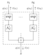
Factor graph for the Algonquin node
Applsci 11 09535 i001
Node function
p ( x s 1 , , s K , γ ) = N x | ln k = 1 K exp ( s k ) , γ 1
MarginalsFunctional form
q ( x ) N x m ^ x , γ ^ x 1 where m ^ x R and γ ^ x R +
q ( s k ) N s k m ^ s k , γ ^ s k 1 where m ^ s k R and γ ^ s k R +
q ( γ ) Γ γ α ^ , β ^ where α ^ , β ^ R +
MessagesFunctional form
ν ( x ) N x | ln k = 1 K exp ( m ^ s k ) , β ^ α ^
ν ( s k ) N s k | m ^ x ln i = 1 K exp ( m s i ) m ^ x σ ( m ^ s ) k , β ^ α ^ σ ( m ^ s ) k 2
ν ( γ ) Γ γ | 3 2 , 1 2 1 γ ^ x + k = 1 K σ ( m ^ s ) k 2 γ ^ s k + m ^ x ln k = 1 K exp ( m ^ s k ) 2
Local variational free energy
1 2 ln ( 2 π ) + 1 2 ψ ( α ^ ) ln ( β ^ ) + α ^ 2 β ^ 1 γ ^ y + k = 1 K σ ( m ^ s ) k 2 γ ^ s k + m ^ x ln k = 1 K exp ( m ^ s k ) 2
Table 2. Table containing (a) the Forney-style factor graph representation of the Gaussian scale sum node. (b) The likelihood function corresponding to the Gaussian scale sum node. (c) An overview of the chosen approximate posterior distributions. Here the · ^ accent refers to the parameters of these distributions. (d) The derived variational messages for the Gaussian scale sum node. (e) The derived local variational free energy. All derivations are available at https://github.com/biaslab/SituatedSoundscaping, accessed on 1 July 2021.
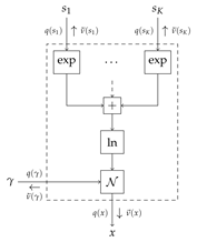
Factor graph for the Gaussian scale sum node
Applsci 11 09535 i002
Node function
p ( x s 1 , , s K ) = N x | 0 , k = 1 K exp ( s k ) , 0
MarginalsFunctional form
q ( x ) N C x m ^ x , γ ^ x 1 , 0 where m ^ x C and γ ^ x R +
q ( s k ) N s k m ^ s k , γ ^ s k 1 where m ^ s k R and γ ^ s k R +
MessagesFunctional form
ν ( x ) N C x | 0 , k = 1 K exp m ^ s k , 0
ν ( s k ) 1 exp ( s k ) + i k exp ( m ^ s i ) exp ( γ ^ x 1 + | m ^ x | 2 ) exp ( s k ) + i k exp ( m ^ s i )
Local variational free energy
ln ( π ) + ln k = 1 K exp ( m ^ s k ) + 1 k = 1 K exp ( m ^ s k ) ( γ ^ x 1 + | m ^ x | 2 )
Publisher’s Note: MDPI stays neutral with regard to jurisdictional claims in published maps and institutional affiliations.

