JUMRv1: A Sentiment Analysis Dataset for Movie Recommendation

Abstract

Nowadays, we can observe the applications of machine learning in every field, ranging from the quality testing of materials to the building of powerful computer vision tools. One such recent application is the recommendation system, which is a method that suggests products to users based on their preferences. In this paper, our focus is on a specific recommendation system called movie recommendation. Here, we make use of user reviews of movies in order to establish a general outlook about the movie and then use that outlook to recommend that movie to other users. However, a huge number of available reviews has baffled sophisticated review systems. Consequently, there is a need to find a method of extracting meaningful information from the available reviews and use that in classifying a movie review and predicting the sentiment in each one. In a typical scenario, a review can either be positive, negative, or indifferent about a movie. However, the available research articles in the field mainly consider this as a two-class classification problem—positive and negative. The most popular work in this field was performed on Stanford and Rotten Tomatoes datasets, which are somewhat outdated. Our work is based on self-scraped reviews from the IMDB website, and we have annotated the reviews into one of the three classes—positive, negative, and neutral. Our dataset is called JUMRv1—Jadavpur University Movie Recommendation dataset version 1. For the evaluation of JUMRv1, we took an exhaustive approach by testing various combinations of word embeddings, feature selection methods, and classifiers. We also analysed the performance trends, if there were any, and attempted to explain them. Our work sets a benchmark for movie recommendation systems that is based on the newly developed dataset using a three-class sentiment classification.

1. Introduction

Because of the psychological nature of reviews, sentiment analysis (SA) of movie reviews is a challenging task for the researchers. SA is the process of manipulating textual media and extracting the subjective value from the text. It determines the review author’s attitude towards a movie: whether it is positive, negative, or indifferent. SA is currently being used all over the internet for various purposes such as political profiling, recommendation engines, fact checking, spam filtering, etc. It has rapidly generated a lot of attention among researchers working with machine learning and Natural Language Processing (NLP), primarily because it takes in crude text from a plethora of sources and transforms it into useful information. With the advent of social media, the amount of data on the internet has boomed. Be it reviews, tweets, comments, poetry, stories, articles, or blogs, these resources can be tapped into and utilised by users. In the industrial sense, SA is mostly used by corporations to get and consider their customers’ feedback. The field of NLP is intertwined with that of SA. Most data on the internet is present in the form of natural text, unrecognizable to the machines due to their complexities and inter-word semantics. NLP is the procedure used in analysing these natural texts in order to form entities that can be understood by the machine for SA. We used various methods to process and classify these movie reviews into one of the three classes—positive, negative, or neutral. The first step in the process was to clean the reviews by removing emojis, punctuation marks, numbers, and stop words that provide no meaningfulness to the text. It is also important to derive the inherent sentiments in that text, which we accomplished by further extracting features out from the texts and using them to classify these texts. Our study included the following steps:

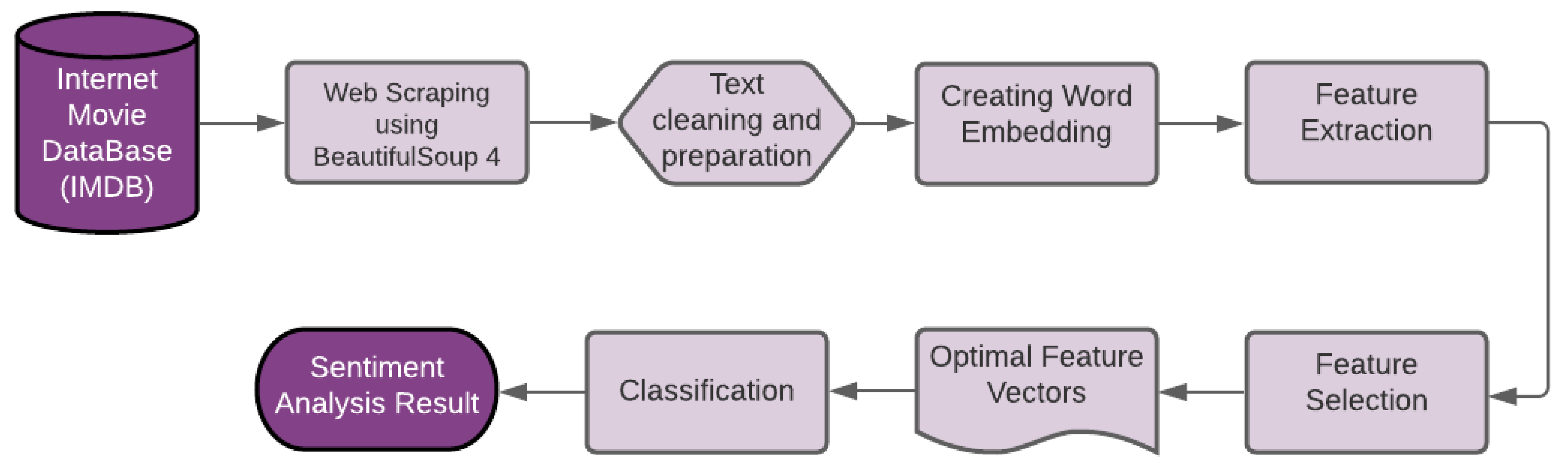
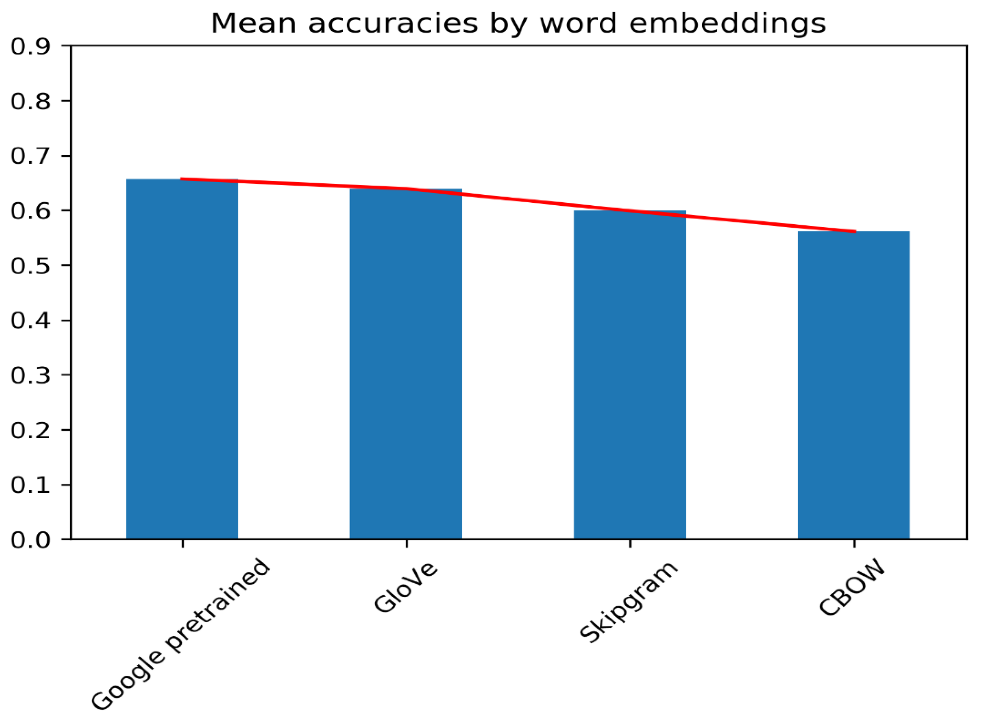
• Word-embedding: We used several word embedding techniques for feature extraction and in order to find the semantics of the words in the cleaned version of the reviews. We used word2vec-skipgram, word2vec-CBOW, Google pre-trained word2vec, and GloVe;
• Feature Selection: By using feature-selection algorithms, we narrowed down the available features to the most important ones. We used three filter methods—Chi-squared, F classifier, Mutual information (MI), and one wrapper method—Recursive Feature Elimination (RFE). All were used with top-k features, where k was optimised;
• Classification: We used three different classifiers with the following methods: Random Forest (RF), XGBoost (XGB), and Support Vector Classifier (SVC).

Our study contributes to the field in a way that it provides noteworthy results to the area of three-class classification with an entirely new database that we freshly scraped from IMDB. We named our dataset JUMRv1—Jadavpur University Movie Recommendation dataset version 1.

The rest of the paper is organised in the following way: Section 2 deals with previous work that has been performed on the topic. Section 3 gives an insight into the dataset that we considered for our study. Section 4 throws light upon the methodology that was followed for the study, a journey from raw data to sentiment classification. Section 5 is a detailed description of the results that we received. Section 6 analyses the results and provides explanations for them. Finally, Section 7 concludes the research, summing it up and providing improvement opportunities.

2. Literature Survey

In the past couple of years, researchers have worked on various recommendation systems based on text data provided by netizens. Baid et al. [1] proposed a study based on the “Sentiment Polarity Dataset version 2.0” from the IMDB website (Pang and Lee [2]), which is a two-class dataset. The classifiers used were Naïve Bayes (NB), K-Nearest Neighbour (KNN), and RF. The word embedding was provided by the StringToWordVector filter. Elghazaly et al. [3] presented a political SA model that used twitter data. They utilised Term Frequency-Inverse Document Frequency (TF-IDF), which is a term weight-based embedding system, combined with simple Naive Bayes (NB) and Support Vector Machine (SVM) classifiers. Pratiwi et al. [4] as well as Adwijaya used document frequency-based vocabulary but implemented feature selection based on information gain. SVM and Neural Network (NN)-based models were used to classify reviews in the the same dataset as Baid et al. [1].

Pang et al. [5] and Lee worked on the SA of IMDB movie review data using unigram, bigram, and uni+bigram models. They used NB, Maximum Entropy, and SVM classifiers to achieve a two-class classification. Tripathy et al. [6] and Zou et al. [7] furthered the work of Pang et al. [5] by adding TF-IDF, POS tagging, and Stochastic Gradient Descent (SGD) in order to improve the accuracies. Ukhti Ikhsani Larasati et al. [8] developed the work of Tripathy et al. [6] and used the chi-squared method of feature selection along with the already proposed SVM classifier.

Ray et al. [9] proposed a hotel recommendation system using a sentiment analysis of the hotel reviews and an aspect-based review categorisation that works on the queries given by a user. They provided a new rich and diverse dataset of online hotel reviews crawled from Tripadvisor.com. They followed a systematic approach, which first used an ensemble of a binary classification called the Bidirectional Encoder Representations from Transformers (BERT) model, with three phases for positive–negative, neutral–negative, and neutral–positive sentiments merged using a weight assigning protocol. The authors also grouped the reviews into different categories using an approach that involved fuzzy logic and cosine similarity. Finally, they created a recommender system with the aforementioned frameworks. Our model achieved a Macro F${}_1$-score of 84% and test accuracy of 92.36% in the classification of sentiment polarities.

Fang and Zhan [10] put forward a product review-based recommendation system from reviews on Amazon.com. Their categorisation was both review-based and sentence-based. Part-of-speech (POS) tagging and sentiment-phrase identification were performed to calculate a sentiment score. These were considered, along with the rating system, which allowed users to rate the product from one-half to five stars. This two-level scoring system was combined with NB, RF, and SVM classifiers.

Barkan and Koenigstein [11] provided an embedding method based on collaborative filtering using the word2vec skip-gram negative sampling method (SGNS) named ‘item2vec’. This was used on a music dataset with artists pertaining to several different genres. When compared to a singular value decomposition classified with a simple KNN model, the embedding resulted in a more accurate score.

Manek et al. [12] used opinion mining based on the Gini index by extracting opinion-oriented words (top 50 words). When performed on several web and self-crawled databases, the result was fed to an SVM classifier. This method does not account for sentences that may contain unopinionated words and yet carry opinions, nor does it deal with sentences that might contain strong polarising words and yet not contain important opinions. Both these works were based on two-class classification.

Liao et al. [13] propounded the use of a deep learning-based classifier along with MR and STS-Gold as the benchmark datasets (Saif et al. [14]) to give a two-class classification. The NN used was CNN, which contained three convolution layers with three max pooling layers, and a softmax layer. The achieved results were better than traditional classifiers such as SVM and NB. Singh et al. [15] put forth a Recurrent Neural Network (RNN)-based multilingual movie recommendation system. A twitter API was used to search for movie details, which provided user comments on the movie. Google maps was used to find the geographical location of the user and the data were translated using Google translator. Afterwards, the data were fed to the Stanford NLP library in order to create the word embedding. An RNN was used to categorise the reviews into positive or negative classes.

Ibrahim et al. [16] used an RNN and Long Short Term Memory (LSTM)-based recommendation model on various datasets such as Twitter, Rotten Tomatoes, etc. Word embedding was provided by SenticNet word network based on the semantics of the words. Uni-gram, bi-gram, and tri-gram texts were fed to the SVM classifier. This model utilises the concept of an LSTM cell, which helps to consider the relationships of a word with words after and before it, providing a better semantic arrangement of words. Wang et al. [17] proposed an “RNN Capsule” method. This method assigns one capsule to each class and uses that capsule’s state and attributes to learn and classify the reviews into positive or negative. This takes away the need for linguistic knowledge by using word embeddings.

Firmanto et al. [18] and Miranda et al. [19] proposed an effective model based on better word embeddings using SentiWordNet. Data from Rotten Tomatoes and Twitter data, respectively, were fed to the SentiWordNet library, which provided a sentiment score for the reviews based on the polarities of specific words present in the library. These scores were then added to find the total, which decides the polarity of the entire review.

In domains related to movie review sentiment analysis, three-class categorization has been a popular subject. Hong et al. [20] provided a three-class sentiment classifier, with book reviews on amazon.com as the corpus. Word2vec word embeddings and several simple and neural-network classifiers were used. Attia et al. [21] propounded a multi-lingual, multi-class sentiment classifier using twitter corpus data for English, German, French, etc. TF-IDF was used along with a CNN for classification. Sharma et al. [22] advanced the work of Liu et al. [23] and proposed an ensemble method for a mutli-class sentiment classifier using SVM and bagging techniques.

3. Dataset

In the present work, we developed a new dataset called JUMRv1, which is to be used in movie recommendation research. We named our dataset in this way as this was prepared in the lab of Jadavpur University, Kolkata, India. Scraped from the Internet Movie Database (https://www.imdb.com/search/title/?title_type=feature,tv_series&count=250&start=001&ref_=adv_nxt, accessed on 10 May 2020), JUMRv1 consists of the top 25 reviews for 60 movies, totalling 1500 reviews. We used the Beautiful Soup 4 library (Richardson [24]) for the scraping. The reviews were annotated as 1, 0, or −1, representing positive, negative, and neutral categories, respectively.

Annotating, though tiresome, is a step of extreme importance as this is going to be reflected in the final dataset that has to be fed to the classifiers. While some reviews were clear and condensed, many reviews were from professional critics who used comprehensive explanations, analogies, and metaphors that were mostly directed at cinema enthusiasts. We ensured constant communication in order to sustain maximum F${}_1$ scores in these annotations. As expected, the annotations revealed some class imbalance. That is, one category outnumbered the others. The class imbalance found in the developed database is as follows (in terms of number):

• Positive (1): 833
• Neutral (0): 301
• Negative (−1): 288

The problem with making natural language datasets is the complexity of human language, with new words creeping into use every day and new semantics arising out of these new words. The addition of the neutral class to the annotation makes the database-making process even more difficult. Some examples taken from JUMRv1 are shown in

Table 1. Examples of movie reviews for each class.

Review	Sentiment	Corresponding Annotation
“Amazing. Steven Spielberg always makes masterpieces…”	Positive	1
“Mediocre performance by Jake Gyllenhaal. The plot is good, worth a watch…”	Neutral	0
“This movie is an utter disaster. This is nothing like the book, full of inaccuracies. A buff batman is unnatural…”	Negative	−1

.

In

Table 2. How JUMRv1 compares to popular movie review datasets.

Dataset	Year of Creation	Year When Last Modified	No. of Reviews	No. of Classes
Polarity Dataset (Cornell)	2002	2004	2000	2
Large Movie Review Dataset (Stanford)	2011	-	50,000	2
Rotten Tomatoes Dataset	2020	-	17,000	2
STS-Gold	2015	2016	2034	2
JUMR v1.0	2021	-	1422	3

, a comparison between the four most popular movie review sentiment analysis datasets and JUMR v1.0 is provided, in terms of when they were last updated, when they were created, how many reviews they hold, and how many classes they have. From this table, it is clearly seen that JUMRv1 holds an advantage over the rest as it provides both comparatively newer movie reviews as well as annotates the reviews into three different classes. On the other hand, the most popular datasets only provide a two-class classification and a rather old set of movies, most of which are irrelevant today.

The dataset has reviews which vary from being sarcastic and ironic to serious and straightforward. This variation of behaviour has resulted in difficulties in the experiments performed to train the classifiers, and has led to a decrease in classification F${}_1$ scores, as seen in the result section. We created a 70:30 train-test split of the dataset for experimentation purposes.

4. Methods and Materials

The methodology that we followed is similar to the one proposed by Sharma and Dey [25]. In our research, the inherent parts include scraping the data from the IMDB website, text pre-processing, creation of a word network, feature extraction, feature selection, and sentiment classification. The workflow of this research is illustrated in Figure 1.

4.1. Pre-Processing

During the creation of JUMRv1, we discovered that textual data in online reviews are written in complex natural human language, which consists of English words (in our case), connector words, different parts of speech, conjunctions, interjections, prepositions, punctuation marks, numbers, emojis, html tags, etc. All these components do not necessarily add value to the text, especially for the SA task. After the web-scraping process, we used the text cleaning method as proposed by Rahman and Hossen [26] in order to clean the reviews. The method is given below:

• Removing non-alphabetic characters, including punctuation marks, numbers, special characters, html tags, and emojis (Garain and Mahata [27]);
• Converting all letters to lower case;
• Removing all words that are less than three characters long as these are not likely to add any value to the review as a whole;
• Removing “stop words” includes words such as “to”, “this”, “for”, as these words do not provide meaning to the review as a whole, and hence will not assist in the processing;
• Normalising numeronyms (Garain et al. [28]);
• Replacing emojis and emoticons with their corresponding meanings (Garain [29]);
• Lemmatising all words to their original form—so that words such as history, historical, and historic—are all converted into their root word: history. This ensures that all these words are processed as the same word; hence, their relations become clearer to the machine. We used the lemmatiser from the spaCy (Honnibal et al. [30]) library.

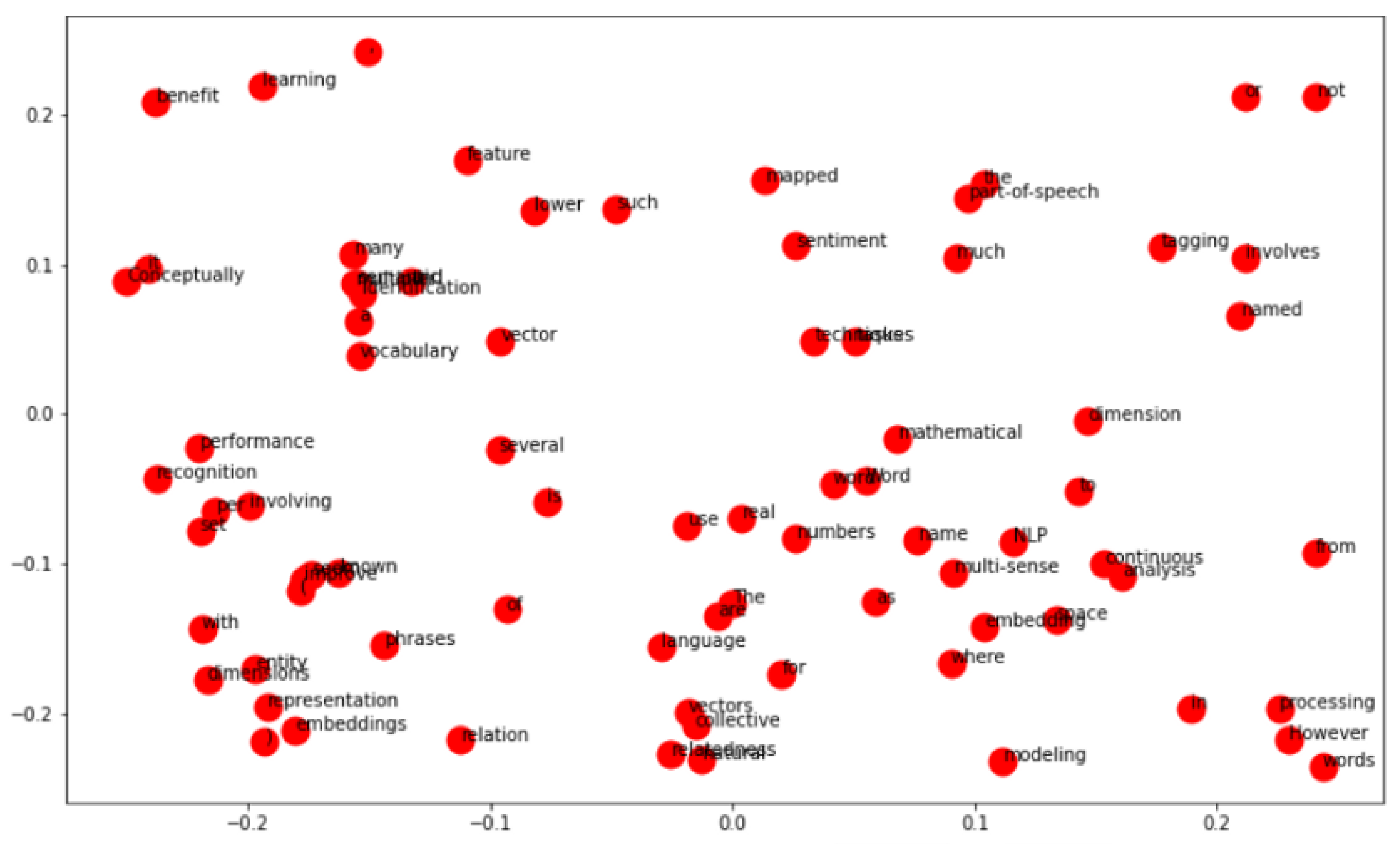
4.2. Word Embedding

Word embedding is a method of representing words in a low-dimensional space, most commonly in the form of real-valued vectors. It allows words with similar meaning and related semantics to be represented closer to each other than less related words. Word embeddings help attach features to all words, depending on their usage in the corpus. In other words, the purpose of word embeddings is to capture inter-word semantics. Figure 2 shows a typical word embedding.

While working on JUMRv1, we dealt with two different approaches to word embeddings, namely Word2Vec and GloVe.

Word2Vec: This is a two-layer NN that vectorises words, hence creating a word embedding. This method works by initialising a random word with a random vector value. It then trains the word according to its neighbouring words in the corpus. Word2Vec models can be customised to have a wide range of vocabularies, a large number of features as well as embedding types. There are also some pre-trained Word2vec models, accessible via open sources (https://towardsdatascience.com/the-three-main-branches-of-word-embeddings-7b90fa36dfb9).

GloVe: GloVe stands for Global Vectors and refers to a method of vectorising all the words given in a corpus while considering global as well as local semantics, unlike Word2Vec, which only takes care of local semantics. This method counts the total number of times one word co-occurs with another word with the use of a co-occurrence matrix; the resultant embedding is made on the basis of relative probabilities.

In this study, we used four different types of word embeddings, three of which are Word2Vec types and one is of the GloVe type. These are the following:

• Google Pre-trained Word2Vec: This is a Word2Vec model, trained by Google on a 100-billion-word Google News dataset and accessed via the gensim library (Mikolov et al. [31]);
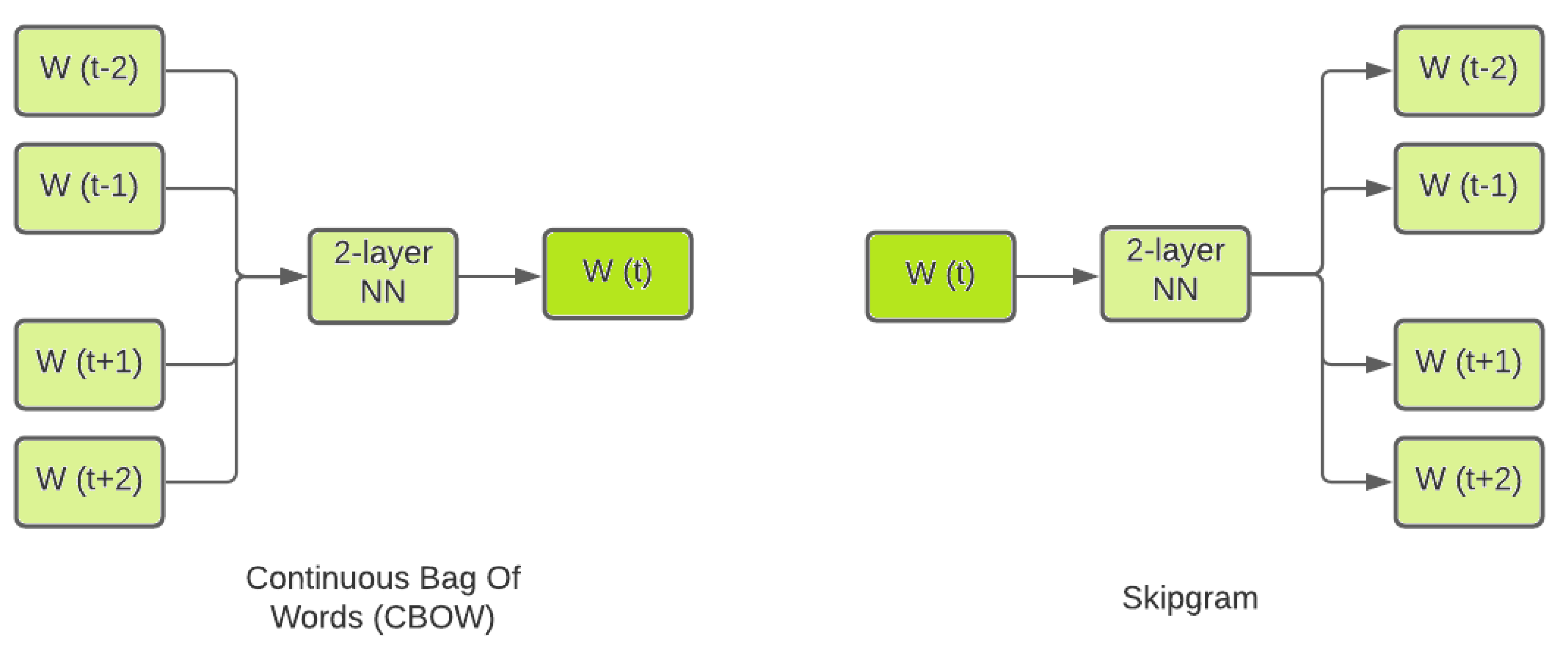
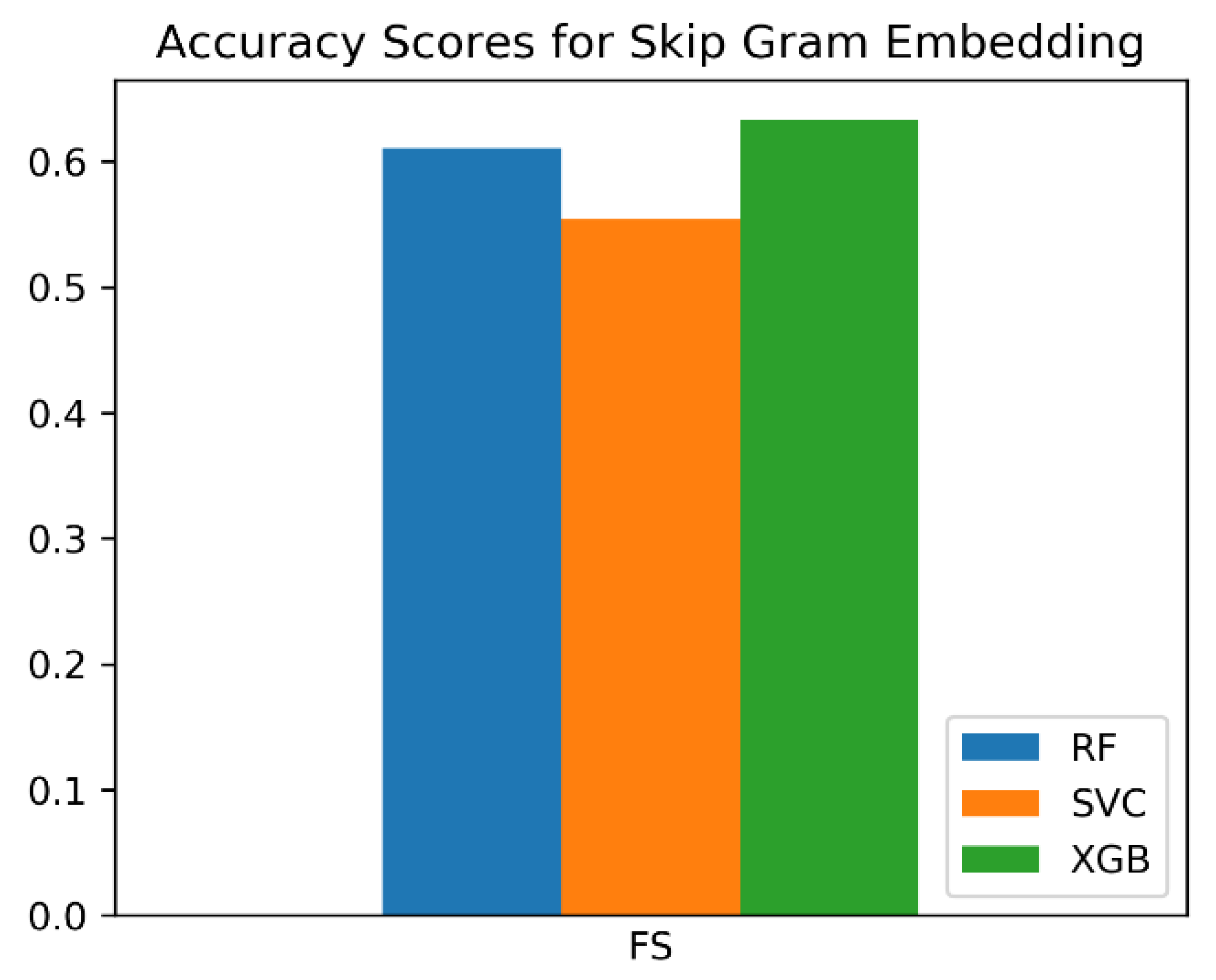
• Custom Word2vec (Skipgram): Here, a custom Word2Vec model that uses “skipgram” neural embedding method is considered. This method relates the central word to the neighbouring words;
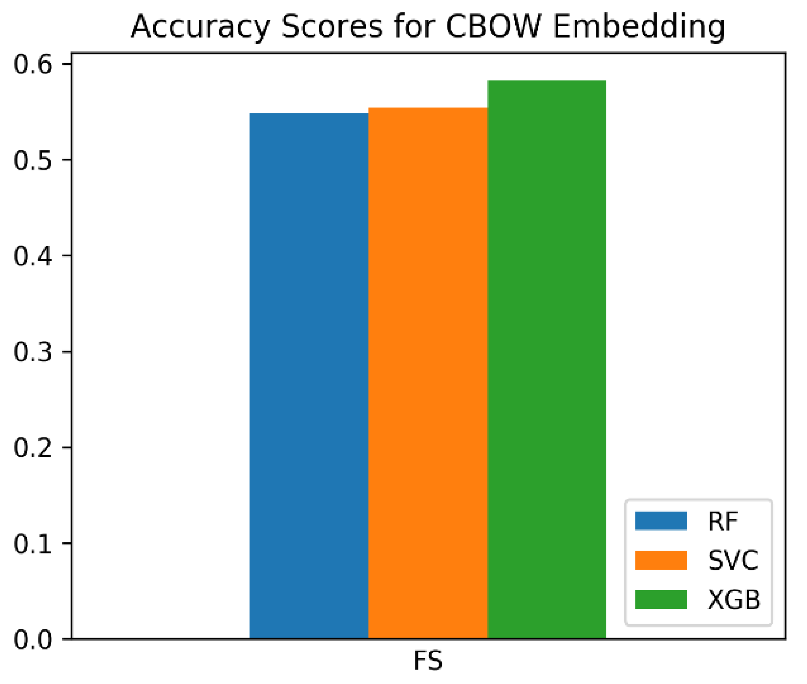
• Custom Word2Vec (Continuous Bag Of Words): Another custom Word2Vec model that uses the Continuous Bag Of Words (CBOW) neural embedding method. This is the opposite of the skipgram model, as this relates the neighbouring words to the central word;
• Stanford University GloVe Pre-trained: This is a GloVe model, trained using Wikipedia 2014 (Pennington et al. [32]) as a corpus by Stanford University, and can be accessed via the university website.

Among these, the first three are Word2Vec-type embeddings and the fourth is a GloVe embedding. Word2Vec embeddings have a neural network that can train itself with two learning models: CBOW and Skipgram.

CBOW: In this method, the representations of the neighbouring (context) words are fed to the NN to predict the word in the middle. The vectors of the context words form the vector of the word in the middle. Error vectors are formed and the individual weights are averaged before passing each word through the softmax layer.

Skipgram: Here, the exact opposite route is taken. The word in the middle is fed to the NN. Error vectors are formed with all words that could possibly be next. The error vectors are calculated and using back propagation, the weights of the hidden layers are updated accordingly. Figure 3 shows a graphical representation of these two methods.

We performed a majority of the exhaustive testings on the Google and Stanford pre-trained embeddings due to the more promising nature of results.

4.3. Feature Extraction

Feature extraction maps the original feature space to a new feature space with a lower or the same number of dimensions by combining the original feature space but with better representation. In our study, we used four word embeddings. Of these four, the Google pre-trained word embedding had 300 features, the GloVe pre-trained embedding had 200 features, and the two Word2Vec embeddings that we trained (Skipgram and CBOW) had 100 features each. Instead of making manual attempts to devise feature vectors for all words in the vocabulary, we took a different approach. We calculated the average embeddings of every word. This can be explained by Equation (1):

$${\overrightarrow{v}}_W=\frac{{\sum }_{iϵW}e\left(W\right)}{\left|W\right|}$$

(1)

where W is a word, ${\overrightarrow{v}}_w$ is the vector for the word, e(W) is the embedding for the word, and $\left|W\right|$ is the total number of words in the vocabulary. Embeddings can be obtained by considering the model function with the word a parameter. These are essentially the coordinates to every word in the multi-dimensional vector space. This contrasts with the otherwise popular method of assigning vectors to packets or entire documents, where the information loss is significant.

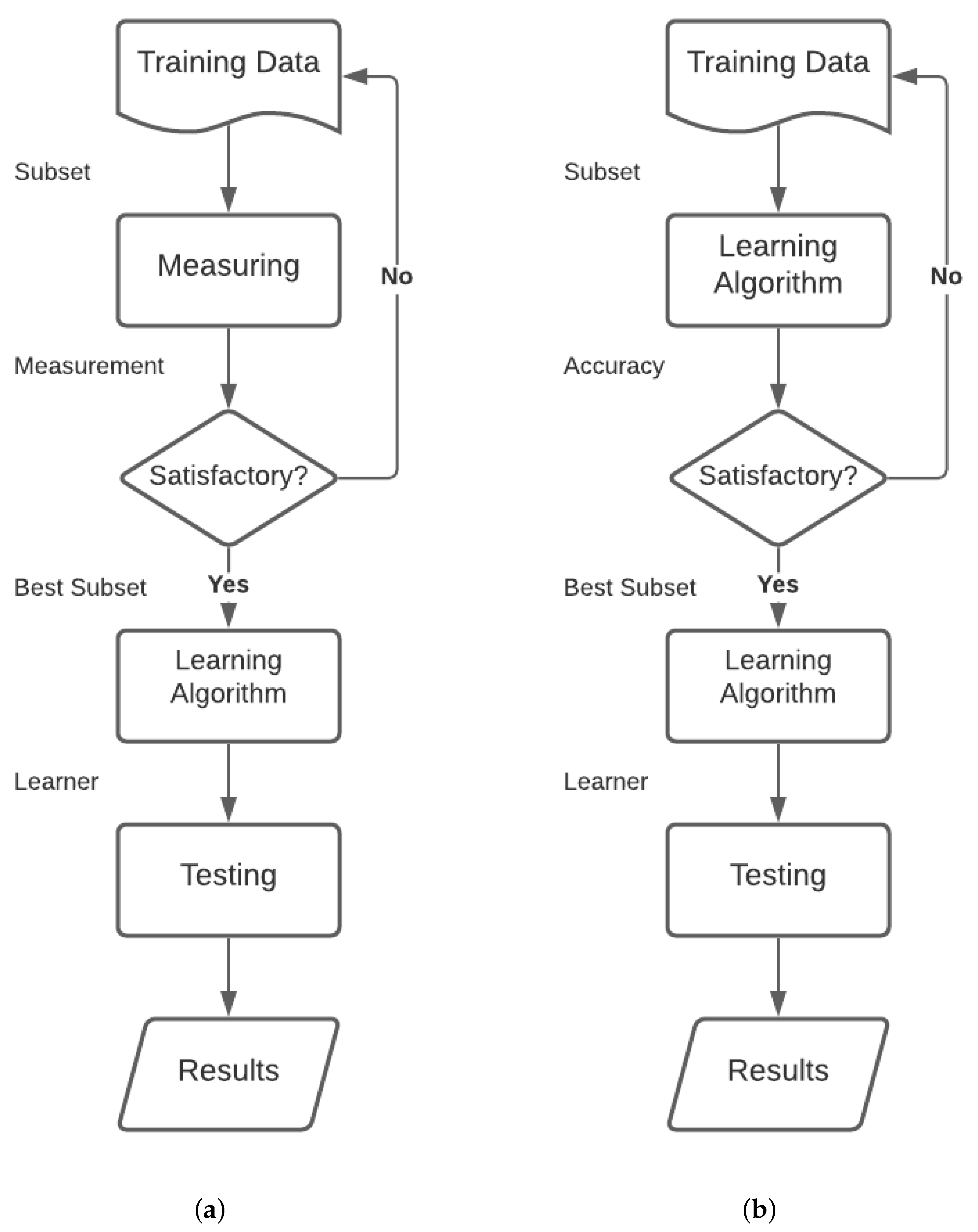
4.4. Feature Selection

Feature selection (Miao and Niu [33]) refers to the process of choosing only the essential features which will have a positive impact on the task of classifying the data into the required labels. Whenever high-dimensional data are used with a lot of features, they often contain some non-informative and redundant features that hamper the process of classification, a phenomenon known as the curse of dimensionality.

It has been documented in the work by Ghosh et al. [34] that not all features are equally important when performing a classification task. Some features seem to have a constructive effect on accuracy, whereas some have a destructive effect. Therefore, we tried to find out if a certain set of features that enhances the accuracy can be selected. According to whether the training set, i.e., features under study, is labelled or not, feature selection algorithms can be categorised into supervised, unsupervised, and semi-supervised feature selection. We used only the supervised feature selection algorithms. The next part deals with the classification of supervised feature selection methods and also describes some of the feature selection methods that were employed in our study. Given below is the classification of feature selection methods based on the selection strategy:

• Filter methods;
• Wrapper Methods;
• Embedded Methods.

The filter method of the feature selection separates feature selection from classifier learning so that the bias of a learning algorithm does not interact with the bias of a feature selection algorithm. It relies on measures of the general characteristics of the training data such as distance, consistency, dependency, information, and correlation. Based on the advantages of filter methods as reported in Ghosh et al. [34], in the present study, we chose three filter-based feature selection methods. We also experimented with one wrapper-based feature selection method. The wrapper model uses the predictive accuracy of a predetermined learning algorithm to determine the quality of selected feature subsets and ultimately to choose the optimal ones. Figure 4 shows the workflow of a feature selection method.

These methods are prohibitively expensive to run for data with a large number of features, but they give commendable results. Given below are the feature selection methods that we used in our study.

4.4.1. Filter Methods

Chi-Squared

Chi-squared is a statistical test that measures the divergence from the expected distribution if the occurrence of a feature is assumed to be independent of the class value (Forman et al. [35]). The chi-squared test measures dependence between stochastic, well-defined variables; hence, using this function eliminates the features that are the most likely to be independent of class and therefore irrelevant for classification. It does so with the use of the chi-squared metric. In the case of continuous variables, the range needs to be divided into intervals (Li et al. [36]). This chi-squared metric, which is also treated as the value of each feature, is given in Equation (2):

$${\chi }_f^2=\sum _{j=1}^r\sum _{s=1}^c{\displaystyle \frac{{(n_{js}-{\mu }_{js})}^2}{{\mu }_{js}}}$$

(2)

where, r is the number of distinct values in the feature, c is the number of distinct values in a class, $n_{js}$ is the frequency of jth element with sth class and ${\mu }_{js}={\displaystyle \frac{n_{*s}{n}_{j*}}{n}}$, $n_{j*}$ is the frequency of jth element, and $n_{*s}$ is the total number of elements with sth class. A higher chi-square value indicates that the feature is more informative.

F-Classifier

This is used to find the Analysis of Variance (ANOVA) f-value. ANOVA can determine whether the means of three or more groups (features in this case) are different. ANOVA uses F-tests to statistically test the equality of means.

F-tests are named after its test statistic. The F-statistic is simply a ratio of two variances. Variances are a measure of dispersion, or how far the data are scattered from the mean. Larger values represent greater dispersion. Dispersed data means the feature will not be that useful because this can be an indication of noise in the data. Therefore, basically, it is used to filter out co-related features.

More importantly, ANOVA is used when one variable is numeric and one is categorical, such as with numerical input variables and a classification target variable in a classification task. The results of this test can be used for feature selection where those features that are independent of the target variable can be removed from the dataset.

Mutual Information

MI is based on the concept of entropy. Entropy is a quantitative measure of how uncertain an event is. This means that if an event has a greater probability of occurring than another, then its entropy is lower than the second event. In classification, MI between two random variables shows dependency between them. Minimum dependency gives zero MI, and as dependency rises, so does the MI.

If $H\left(X\right)$, $H\left(Y\right)$, and $H(X;Y)$ are the entropies of X, Y, and the joint entropy of X and Y, then mutual information between X and Y can be defined as shown in Equation (3):

$$MI(X;Y)=H\left(X\right)+H\left(Y\right)-H(X;Y)$$

(3)

The mutual information between two discreet variables X and Y is given as shown in Equation (4):

$$MI(X;Y)=\sum _{yϵY}\sum _{xϵX}{p}_{(X,Y)}(x,y)log(\frac{p_{(X,Y)}(x,y)}{p_X\left(x\right)p_Y\left(y\right)})$$

(4)

where $p_{X,Y}$ is the joint probability density function for X and Y, and $p_X$ and $p_Y$ are the marginal probability density functions for X and Y, respectively. MI is calculated between two variables by testing the reduction in uncertainty of one variable, given a fixed value for the other. If MI does not exceed a given threshold, that feature is removed. This method can be used for both numerical and categorical data.

4.4.2. Wrapper-Based Method

Recursive Feature Elimination

Given an external estimator that assigns weights to features (e.g., the coefficients of a linear model), the goal of RFE is to select features by recursively considering smaller and smaller sets of features. First, the estimator is trained on the initial set of features and the importance of each feature is obtained either through any specific attribute (such as coef_, feature_importances_) or callable. Then, the least important features are pruned from the current set of features. That procedure is recursively repeated on the pruned set until the desired number of features with optimal accuracy is eventually reached.

4.5. Classification

We incorporated three standard classifiers into the three-class classification task under consideration, for each of the combinations of embedding and feature selection mechanisms.

4.5.1. Random Forest

This is a bagging-type classifier and it is essentially an ensemble of individual decision trees. It incorporates a number of decision tree classifiers, trains them over various sub-samples of the dataset, and uses averaging to increase the predictive accuracy. The fundamentals behind the functions of a random forest classifier is that when a number of independent and uncorrelated decision trees work as a voted ensemble, they outperform all of these individual models. Because of this low correlation, there is randomness among these models.

4.5.2. XGBoost

XGBoost stands for eXtreme Gradient Boosting. Unlike the bagging technique that merges similar decision-making classifiers together, XGB is a boosting-type ensemble algorithm. Boosting is a sequential ensemble that uses different iterations to remove misclassified observations by increasing their weights with every iteration. Boosting keeps track of the learner’s errors. Using parameters to control the maximum depth of decision trees being used and the number of classes in the dataset, the XGB model can be used to deal with data that have a large variance. Boosting is completed sequentially instead of parallelly such as in bagging methods.

4.5.3. Support Vector Classifier

This algorithm is completely different from the previous two, as its fundamentals involve finding a hyperplane in an N-dimensional space. The target is to maximise the support vectors.

Decision Boundary: This is a hyperplane that separates different classes of observations. The dimensionality of a hyperplane depends on that of the data. This simply means that for two-feature $R^2$ data, a hyperplane is a line, and for three-feature $R^3$ data, it is a plane.

Support Vector: Support vectors are observations that lie closest to the decision boundary that influences its position and directionality. In the proposed study, SVC has been used via the scikit-learn package with the Radial Basis Function (RBF) kernel. These kernels are specified for hyperplanes that are non-linear, as real world data do not necessarily need to be linear.

5. Results and Discussion

As mentioned earlier, in this work, we prepared a three-class SA dataset called JUMRv1 for the development of movie recommendation systems. We also provided the required annotation so that other researchers can assess the performance of their methods. To set a benchmark result on JUMRv1, we performed an exhaustive set of experiments. After extensive testing with different word embeddings and feature selection methods, as well as with the SVC, RF, and XGB classifiers, the SA results have been categorised and are discussed below.

GloVe (Pennington et al. [32]) word embedding, developed by Stanford University Researchers, was trained on the entire Wikipedia corpus. It was used as a stand-alone with all 200 of its available features and along with different feature selection methods, which were utilised to rank the importance of the features, employing 150, 100, and 50 of these in the experiments.

5.1. Analysis Metrics

In order to analyse the performance of our model on various datasets, we considered the standard performance metrics, namely the F${}_1$ score and the accuracy score with their corresponding class support division.

Precision is defined as:

$${\displaystyle \mathrm{Precision}=\frac{\mathrm{TP}}{\mathrm{TP}+\mathrm{FP}}}$$

(5)

Recall is defined as:

$${\displaystyle \mathrm{Recall}=\frac{\mathrm{TP}}{\mathrm{TP}+\mathrm{FN}}}$$

(6)

Accuracy score is defined as:

$${\displaystyle \mathrm{Accuracy}-\mathrm{score}=\frac{\mathrm{TP}+\mathrm{TN}}{\mathrm{TP}+\mathrm{TN}+\mathrm{FP}+\mathrm{FN}}}$$

(7)

Here, TP (True Positive) = Number of reviews correctly classified into corresponding sentiment classes.

FP (False Positive) = Number of reviews classified as belonging to a sentiment class that they do not belong to.

FN (False Negative) = Number of reviews classified as not belonging to a sentiment class that they actually belong to.

The F${}_1$ score is defined as:

$${\displaystyle {\mathrm{F}}_1-\mathrm{score}=2\times \frac{\mathrm{Precision}\times \mathrm{Recall}}{(\mathrm{Precision}+\mathrm{Recall})}}$$

(8)

Support for a sentiment class is defined as the number of reviews that lies in that sentiment class.

Figure 5 shows the F${}_1$ scores that we obtained using GloVe word embeddings with 200 features (i.e., no feature selection).

Table 3. F₁ scores obtained by using GloVe pre-trained embeddings and selecting 150, 100, and 50 features.

Feature Selection	Features Selected	Classifier	F1-Score
Recursive (RF)	150	RF	0.6667
Recursive (RF)		XGB	0.6667
Recursive (RF)		SVC	0.6045
Recursive (XGB)		RF	0.6384
Recursive (XGB)		XGB	0.6384
Recursive (XGB)		SVC	0.5593
Chi-Squared		RF	0.6158
Chi-Squared		XGB	0.7006
Chi-Squared		SVC	0.6441
Mutual Info		RF	0.6441
Mutual Info		XGB	0.661
Mutual Info		SVC	0.5593
F Classifier		RF	0.6441
F Classifier		XGB	0.6667
F Classifier		SVC	0.565
Recursive (RF)	100	RF	0.6553
Recursive (RF)		XGB	0.6327
Recursive (RF)		SVC	0.6158
Recursive (XGB)		RF	0.644
Recursive (XGB)		XGB	0.644
Recursive (XGB)		SVC	0.5593
Chi-Squared		RF	0.644
Chi-Squared		XGB	0.6836
Chi-Squared		SVC	0.6666
Mutual Info		RF	0.6779
Mutual Info		XGB	0.6836
Mutual Info		SVC	0.5649
F Classifier		RF	0.6497
F Classifier		XGB	0.6892
F Classifier		SVC	0.5649
Recursive (RF)	50	RF	0.644
Recursive (RF)		XGB	0.6779
Recursive (RF)		SVC	0.6214
Recursive (XGB)		RF	0.649717
Recursive (XGB)		XGB	0.649715
Recursive (XGB)		SVC	0.6271
Chi-Squared		RF	0.6779
Chi-Squared		XGB	0.6723
Chi-Squared		SVC	0.6666
Mutual Info		RF	0.644
Mutual Info		XGB	0.6836
Mutual Info		SVC	0.5932
F Classifier		RF	0.6892
F Classifier		XGB	0.6553
F Classifier		SVC	0.6327

denotes the F${}_1$ scores received via Glove embeddings, but with the help of different feature selection methods, selecting 150, 100, and 50 of the most important features.

Google Word2Vec word embedding is one of the most popular embeddings used in NLP. Here, we used the Word2Vec pre-trained model, which was trained on the Google News corpus with 100 billion words in its vocabulary. It has 300 features and using different feature selection methods, we ranked these features and selected the top 150, 100, and 50 features accordingly.

Figure 6 shows the F${}_1$ scores for Google’s pre-trained Word2Vec embedding with all 300 features (i.e., no feature selection).

Table 4. F₁ scores obtained by using Google pre-trained Word2Vec embedding and selecting 150, 100, and 50 features.

Feature Selection	Features Selected	Classifier	F1 Score
Recursive (RF)	150	RF	0.6667
Recursive (RF)		XGB	0.6667
Recursive (RF)		SVC	0.6045
Recursive (XGB)		RF	0.6384
Recursive (XGB)		XGB	0.6384
Recursive (XGB)		SVC	0.5593
Chi-Squared		RF	0.6158
Chi-Squared		XGB	0.7006
Chi-Squared		SVC	0.6441
Mutual Info		RF	0.6441
Mutual Info		XGB	0.661
Mutual Info		SVC	0.5593
F Classifier		RF	0.6441
F Classifier		XGB	0.6667
F Classifier		SVC	0.565
Recursive (RF)	100	RF	0.6723
Recursive (RF)		XGB	0.6949
Recursive (RF)		SVC	0.6723
Recursive (XGB)		RF	0.6553
Recursive (XGB)		XGB	0.6553
Recursive (XGB)		SVC	0.6949
Chi-Squared		RF	0.661
Chi-Squared		XGB	0.6497
Chi-Squared		SVC	0.6949
Mutual Info		RF	0.6497
Mutual Info		XGB	0.6271
Mutual Info		SVC	0.6271
F Classifier		RF	0.6497
F Classifier		XGB	0.6836
F Classifier		SVC	0.6666
Recursive (RF)	50	RF	0.661
Recursive (RF)		XGB	0.6949
Recursive (RF)		SVC	0.712
Recursive (XGB)		RF	0.678
Recursive (XGB)		XGB	0.678
Recursive (XGB)		SVC	0.7006
Chi-Squared		RF	0.695
Chi-Squared		XGB	0.6892
Chi-Squared		SVC	0.6892
Mutual Info		RF	0.7006
Mutual Info		XGB	0.6441
Mutual Info		SVC	0.6497
F Classifier		RF	0.6836
F Classifier		XGB	0.6271
F Classifier		SVC	0.6836

shows the F₁ scores obtained on the same embedding upon selection of the top 150, 100, and 50 features.

We also trained the Word2Vec model on our own data corpus using the CBOW approach once and the Skipgram approach once. The three classifiers—SVC, RF, and XGB—were also used here. Although the F${}_1$ scores were not that promising, they still gave us important insights about the data. The results are given in

Table 5. Embeddings: Custom CBOW, Skipgram, Word2Vec (trained by our group). Features: 100.

Embedding	Classifier	F1 Score
CBOW	RF	0.54802
CBOW	XGB	0.58192
CBOW	SVC	0.55367
Skipgram	SVC	0.55367
Skipgram	RF	0.61017
Skipgram	XGB	0.63277

.

In

Table 6. Confusion matrix for Glove embedding with the RFE(RF) feature selection method; 50 features.

26	6	16
5	4	22
2	5	91

,

Table 7. Confusion matrix for Glove Embedding with feature selection method of F Classifier, 100 features.

26	3	19
5	3	23
3	2	93

,

Table 8. Confusion matrix for Glove embedding with the RFE(RF) feature selection method; 100 features.

25	4	19
3	2	26
3	1	94

,

Table 9. Confusion matrix for Glove embedding with the Chi-squared feature selection method; 100 features.

25	4	19
3	2	26
3	1	94

,

Table 10. Confusion matrix for Glove embedding with F Classifier feature selection method and 100 features.

28	4	16
5	4	22
2	6	90

,

Table 11. Confusion matrix for Glove embedding with the RFE (RF) feature selection method; 150 features.

24	5	19
5	5	21
2	3	93

,

Table 12. Confusion matrix for Glove embedding with the Chi-Squared feature selection method; 150 features.

25	6	17
6	5	20
1	3	94

,

Table 13. Confusion matrix for Word2Vec embedding with the RFE (RF) feature selection method; 100 features.

26	8	14
4	5	22
2	3	93

,

Table 14. Confusion matrix for Glove embedding with the RFE (RF) feature selection method; 150 features.

24	5	19
5	5	21
2	3	93

and

Table 15. Confusion matrix for Word2Vec embedding with the RFE (RF) feature selection method; 150 features.

24	5	19
5	5	21
2	3	93

, confusion matrices are given for the 10 most accurate models that we achieved, along with their precision and recall values. The classifier used for Table 6 is XGB, with an accuracy score of 0.6836 and the precision and recall being 0.6838 and 0.683, respectively. The F₁ score is 0.66. The classifier used in Table 7 is the Random Forest Classifier, with an accuracy score of 0.689, precision of 0.689, recall of 0.689, and an F₁ score of 0.689. The classifier used in Table 8 is the Random Forest Classifier with an accuracy score of 0.6836, precision of 0.6836, recall of 0.666, and an F₁ score of 0.675. The classifier used in Table 9 is XGB, with an accuracy score of 0.6836, precision of 0.6836, recall of 0.666, and an F₁ score of 0.675. The classifier used in Table 10 is XGB, with an accuracy score of 0.689, precision of 0.68, recall of 0.686, and an F₁ score of 0.682. The classifier used in Table 11 is XGB, with an accuracy score of 0.6892, precision of 0.664, recall of 0.672, and an F₁ score of 0.668. The classifier used in Table 12 is XGB, with an accuracy score of 0.7005, precision of 0.7, recall of 0.7, and an F₁ score of 0.7. The classifier used in Table 13 is XGB, with an accuracy score of 0.7, precision of 0.7, recall of 0.68, and an F₁ score of 0.69. The classifier used in Table 14 is SVC, with an accuracy score of 0.695, precision of 0.694, recall of 0.687, and an F₁ score of 0.69. The classifier used in Table 15 is XGB, with an accuracy score of 0.6892, precision of 0.664, recall of 0.672, and an F₁ score of 0.668.

The visual representation of the entire exhaustive testing procedure, marking all the different embeddings, feature selection methods, and classifiers are shown in Figure 7, Figure 8, Figure 9, Figure 10 and Figure 11.

Figure 8 shows a similar exhaustive testing for the Google pre-trained embedding on the dataset.

Figure 9 shows the F${}_1$ scores of all three classifiers on the CBOW Word2Vec database that we trained.

Figure 10 shows the F${}_1$ scores of all three classifiers on the Skipgram Word2Vec database that we trained.

Figure 11 lists the means of the F${}_1$ scores for all observations on the four word embeddings.

5.2. Software Used

To set a benchmark result for JUMRv1—the newly developed SA-based movie recommender dataset, we performed various experiments. For the purpose of implementation, we used different software: We used NumPy (Harris et al. [37]) and Pandas (pandas development team [38]) for Array and DataFrame operations. The web-scraper that we used to prepare the JUMRv1 can be found in the Beautiful Soup (Richardson [24]) library. For text cleaning, we used Regular Expression (Van Rossum [39]), and for the lemmatisation, the SpaCy Lemmatizer (Honnibal et al. [30]). To create the word embeddings, the Gensim (Řehůřek and Sojka [40]) library was used for both Google’s pre-trained and our self-trained Word2Vec, while GloVe (Pennington et al. [32]) had to be downloaded from the Stanford website. For the feature selection and classification methods, Scikit-Learn (Pedregosa et al. [41]) was used. All graphical visualisations were performed using MatPlotLib (Hunter [42]).

6. Analysis

An analysis of the aforementioned results indicates the following trends:

As we increased the number of features fed to the classifiers, F${}_1$ scores of the SVCs seemed to dropped. This is apparent from Figure 7 and Figure 8. This leads to two conclusions. First, the samples in the dataset are dispersed, and the degree of dispersion (scatter) is notable. A statistical measure of scatter is the variance. High variance has led to the underfitting of the SVC, and as the number of features is increased, the underfitting increases as well. A plausible solution is the proper scaling of the data around the mean. This again serves as a trade-off as scaling might sometimes lead to information loss, which does not reflect the real-life data, especially in the case of embeddings with vocabularies as large as ours.

With fewer features, the decision boundary hyperplanes that are formed become simpler. Therefore, hyperplanes with 50 features and 100 features are much simpler than those with 150 features, pertaining to the fact that an increase in feature numbers leads to an increase in the complexity of hyperplane decision boundaries.

As seen in Figure 7 and Figure 8, when we increased the number of features, almost all XGB classifiers improved their F${}_1$ scores, while with fewer features, RF had better F${}_1$ scores. This can be attributed to the bias–variance trade-off. RF is more robust against overfitting and carries a low bias. At the same time, it does not work well with high variance. XGB, however, improves the bias and is hence less affected by the increase in variance as the number of features increase. It is also susceptible to overfitting.

As is apparent from Figure 7 and Figure 8, SVCs behaved marginally better with the Google pre-trained Word2Vec embedding (at par with RF and XGB), than with the GloVe pre-trained embedding. Word2Vec is an NN-based method that predicts the placement of one word with respect to the other words. GloVe, however, operates via two co-occurrence matrices and its fundamentals are frequency-of-use-based and not predictive. With a relatively small vocabulary of about two thousand words, Word2Vec has worked well with complex mathematical SVCs; an embedded word vector also directly implies simpler hyperplanes.

In Table 3, we see that among the available feature selection methods, Chi-squared and RF gave the highest F${}_1$ scores. The chi-squared test is a statistical test that determines if one variable is independent of another. It uses the chi-squared statistic as a measure. RF, on the other hand, is an ensemble of decision trees that are used to classify specified classes. While the chi-squared method is a hypothesis-driven method, RF is centred around decision trees. Both these methods are prone to noisy data but perform exceptionally well with smaller datasets with a more finite corpus such as ours.

A simple look at Figure 11 reveals that feature selection methods gave much more prominent results with Google’s pre-trained Word2Vec embedding than with the GloVe pre-trained embedding. The reason for this is similar to that of a previous observation: Word2Vec being an NN-based embedding, it can attain better semantics even with a smaller dataset; on the other hand, GloVe, which is majorly dependent upon co-occurrence, fails to do so. Hence, it is worth noting that the semantics captured by the Google pre-trained Word2Vec embedding are superior to those captured by the GloVe pre-trained embedding. Another prominent reason is that the GloVe embedding was based on a corpus of articles that have now become outdated and do not bring as much context to a movie review dataset as Google’s Word2Vec does. Figure 11 clearly shows that the embeddings that have been trained here, namely the Word2Vec Skipgram and the Word2Vec CBOW, provided results that are not as accurate as those provided by the Google Word2Vec and GloVe embeddings. The Google and GloVe word embeddings were trained on huge datasets with vocabularies of up to 100 billion words. With better vocabularies and a larger corpus, word semantics were better captured in these word embeddings. In contrast, our corpus had a fraction of those words. This led to appreciably less semantic word embeddings and consequentially, lower F${}_1$ scores. A simple remedy is to use a larger corpus to avoid any such cold start scenarios.

All the observations from Figure 11 were below the standard results. With the leading and average F${}_1$ scores in the two-class category being 0.9742 (as recorded in Thongtan and Phienthrakul [43]) and 0.93 (in Yasen and Tedmori [44]), the F${}_1$ scores achieved in our studies seem sub-standard. Firstly, our dataset is much smaller compared to the popular datasets used in the field. Secondly, a three-class classification is much more complex than a two-class classification. This is made even more complex by the imbalance we have in the dataset, which cannot be removed due to the persistent cold start.

7. Conclusions

In this paper, we studied the problem of movie recommendation systems, where we considered online movie reviews in order to suggest movies to people. We proposed a dataset called JUMRv1 for the development of movie recommendation systems using three-class SAs and performed an exhaustive experimentation of various models to present the baseline results of the overall sentiment of the reviews. In order to develop this database, we crawled, annotated, and cleaned the reviews taken from the popular movie review website called IMDB. To the best of our knowledge, all popular research works on movie recommendation systems have been performed considering these as a two-class classification problem and with the use of older datasets. The novelty of our research is that it provides a large-scale dataset, with a high number of reviews as well as reviews for newer movies, which bring into context some words and phrases that pertain to the newest trends. It brings more realism into the field of movie review sentiment analysis as it is only natural for people to have indifferent opinions on movies. A wider range of sentiments makes the dataset more applicable to the real world. Our research paves the way for further research into the field of three-class sentiment classification for movie reviews.

Although these results are a cornerstone in the testing of the respective methods, the F₁ scores that we achieved are significantly below the industry standard. The reasons are highly related to the length, class-imbalance, and complexity of the dataset, which provides us with the opportunity for improvement. Future work on JUMRv1 can explore other feature extraction techniques such as the use of transformers and the n-gram methodology. Subsequently, other ensemble methods can be used for further investigation on increasing classification metrics. As seen in Section 3, there is clearly an imbalance in the data. The dataset is almost completely positively biased, and it is not easy to remove that imbalance. Further improvement can be made by adding more negative and indifferent reviews. It would not only help the models train better, but will also provide more varieties to the word embeddings generated. It is always possible to add more reviews to the dataset, which would make it larger and hence provide us with more test and train data samples. As we have performed a general sentiment analysis here, we can leverage the dataset for multi-target-based sentiment analyses and execute an exhaustive set of experiments for the same, pertaining to the fact that the annotation may still be extended to further enhance on our dataset.

References

1. Baid, P.; Gupta, A.; Chaplot, N. Sentiment analysis of movie reviews using machine learning techniques. Int. J. Comput. Appl. 2017, 179, 45–49. [Google Scholar] [CrossRef]
2. Pang, B.; Lee, L. A Sentimental Education: Sentiment Analysis Using Subjectivity Summarization Based on Minimum Cuts. arXiv 2004, arXiv:cs/0409058. [Google Scholar]
3. Elghazaly, T.; Mahmoud, A.; Hefny, H.A. Political sentiment analysis using twitter data. In Proceedings of the International Conference on Internet of things and Cloud Computing, Cambridge, UK, 23 February—22 March 2016; pp. 1–5. [Google Scholar]
4. Pratiwi, A.I. On the feature selection and classification based on information gain for document sentiment analysis. Appl. Comput. Intell. Soft Comput. 2018, 2018, 1407817. [Google Scholar] [CrossRef] [Green Version]
5. Pang, B.; Lee, L.; Vaithyanathan, S. Thumbs up? Sentiment classification using machine learning techniques. arXiv 2002, arXiv:cs/0205070. [Google Scholar]
6. Tripathy, A.; Agrawal, A.; Rath, S.K. Classification of sentiment reviews using n-gram machine learning approach. Expert Syst. Appl. 2016, 57, 117–126. [Google Scholar] [CrossRef]
7. Zou, H.; Tang, X.; Xie, B.; Liu, B. Sentiment classification using machine learning techniques with syntax features. In Proceedings of the 2015 International Conference on Computational Science and Computational Intelligence (CSCI), Las Vegas, NV, USA, 7–9 December 2015; pp. 175–179. [Google Scholar]
8. Ukhti Ikhsani Larasati, I.U.; Much Aziz Muslim, I.U.; Riza Arifudin, I.U.; Alamsyah, I.U. Improve the Accuracy of Support Vector Machine Using Chi Square Statistic and Term Frequency Inverse Document Frequency on Movie Review Sentiment Analysis. Sci. J. Inform. 2019, 6, 138–149. [Google Scholar]
9. Ray, B.; Garain, A.; Sarkar, R. An ensemble-based hotel recommender system using sentiment analysis and aspect categorization of hotel reviews. Appl. Soft Comput. 2021, 98, 106935. [Google Scholar] [CrossRef]
10. Fang, X.; Zhan, J. Sentiment analysis using product review data. J. Big Data 2015, 2, 5. [Google Scholar] [CrossRef] [Green Version]
11. Barkan, O.; Koenigstein, N. Item2vec: Neural item embedding for collaborative filtering. In Proceedings of the 2016 IEEE 26th International Workshop on Machine Learning for Signal Processing (MLSP), Salerno, Italy, 13–16 September 2016; pp. 1–6. [Google Scholar]
12. Manek, A.S.; Shenoy, P.D.; Mohan, M.C.; Venugopal, K. Aspect term extraction for sentiment analysis in large movie reviews using Gini Index feature selection method and SVM classifier. World Wide Web 2017, 20, 135–154. [Google Scholar] [CrossRef] [Green Version]
13. Liao, S.; Wang, J.; Yu, R.; Sato, K.; Cheng, Z. CNN for situations understanding based on sentiment analysis of twitter data. Procedia Comput. Sci. 2017, 111, 376–381. [Google Scholar] [CrossRef]
14. Saif, H.; Fernandez, M.; He, Y.; Alani, H. Evaluation datasets for Twitter sentiment analysis: A survey and a new dataset, the STS-Gold. In Proceedings of the 1st Interantional Workshop on Emotion and Sentiment in Social and Expressive Media: Approaches and Perspectives from AI (ESSEM 2013), Turin, Italy, 3 December 2013. [Google Scholar]
15. Singh, T.; Nayyar, A.; Solanki, A. Multilingual opinion mining movie recommendation system using RNN. In Proceedings of First International Conference on Computing, Communications, and Cyber-Security (IC4S 2019); Springer: Berlin/Heidelberg, Germany, 2020; pp. 589–605. [Google Scholar]
16. Ibrahim, M.; Bajwa, I.S.; Ul-Amin, R.; Kasi, B. A neural network-inspired approach for improved and true movie recommendations. Comput. Intell. Neurosci. 2019, 2019, 4589060. [Google Scholar] [CrossRef] [PubMed] [Green Version]
17. Wang, Y.; Sun, A.; Han, J.; Liu, Y.; Zhu, X. Sentiment analysis by capsules. In Proceedings of the 2018 World Wide Web Conference, Lyon, France, 23–27 April 2018; pp. 1165–1174. [Google Scholar]
18. Firmanto, A.; Sarno, R. Prediction of movie sentiment based on reviews and score on rotten tomatoes using sentiwordnet. In Proceedings of the 2018 International Seminar on Application for Technology of Information and Communication, Semarang, Indonesia, 21–22 September 2018; pp. 202–206. [Google Scholar]
19. Miranda, E.; Aryuni, M.; Hariyanto, R.; Surya, E.S. Sentiment Analysis using Sentiwordnet and Machine Learning Approach (Indonesia general election opinion from the twitter content). In Proceedings of the 2019 International Conference on Information Management and Technology (ICIMTech), Denpasar, Indonesia, 19–20 August 2019; Volume 1, pp. 62–67. [Google Scholar]
20. Hong, J.; Nam, A.; Cai, A. Multi-Class Text Sentiment Analysis. 2019. Available online: http://cs229.stanford.edu/proj2019aut/data/assignment_308832_raw/26644050.pdf (accessed on 29 September 2021).
21. Attia, M.; Samih, Y.; Elkahky, A.; Kallmeyer, L. Multilingual multi-class sentiment classification using convolutional neural networks. In Proceedings of the Eleventh International Conference on Language Resources and Evaluation (LREC 2018), Miyazaki, Japan, 7–12 May 2018. [Google Scholar]
22. Sharma, S.; Srivastava, S.; Kumar, A.; Dangi, A. Multi-Class Sentiment Analysis Comparison Using Support Vector Machine (SVM) and BAGGING Technique-An Ensemble Method. In Proceedings of the 2018 International Conference on Smart Computing and Electronic Enterprise (ICSCEE), Kuala Lumpur, Malaysia, 11–12 July 2018; pp. 1–6. [Google Scholar]
23. Liu, Y.; Bi, J.W.; Fan, Z.P. Multi-class sentiment classification: The experimental comparisons of feature selection and machine learning algorithms. Expert Syst. Appl. 2017, 80, 323–339. [Google Scholar] [CrossRef] [Green Version]
24. Richardson, L. Beautiful Soup Documentation. 2007. Available online: https://beautiful-soup-4.readthedocs.io/en/latest/ (accessed on 29 September 2021).
25. Sharma, A.; Dey, S. Performance investigation of feature selection methods and sentiment lexicons for sentiment analysis. IJCA Spec. Issue Adv. Comput. Commun. Technol. HPC Appl. 2012, 3, 15–20. [Google Scholar]
26. Rahman, A.; Hossen, M.S. Sentiment analysis on movie review data using machine learning approach. In Proceedings of the 2019 International Conference on Bangla Speech and Language Processing (ICBSLP), Sylhet, Bangladesh, 27–28 September 2019; pp. 1–4. [Google Scholar]
27. Garain, A.; Mahata, S.K. Sentiment Analysis at SEPLN (TASS)-2019: Sentiment Analysis at Tweet Level Using Deep Learning. arXiv 2019, arXiv:1908.00321. [Google Scholar]
28. Garain, A.; Mahata, S.K.; Dutta, S. Normalization of Numeronyms using NLP Techniques. In Proceedings of the 2020 IEEE Calcutta Conference (CALCON), Kolkata, India, 28–29 February 2020; pp. 7–9. [Google Scholar]
29. Garain, A. Humor Analysis Based on Human Annotation (HAHA)-2019: Humor Analysis at Tweet Level Using Deep Learning. 2019. Available online: https://www.researchgate.net/publication/335022260_Humor_Analysis_based_on_Human_Annotation_HAHA-2019_Humor_Analysis_at_Tweet_Level_using_Deep_Learning (accessed on 29 September 2021).
30. Honnibal, M.; Montani, I.; Van Landeghem, S.; Boyd, A. spaCy: Industrial-Strength Natural Language Processing in Python. 2020. Available online: https://spacy.io/ (accessed on 29 September 2021). [CrossRef]
31. Mikolov, T.; Chen, K.; Corrado, G.; Dean, J. Efficient estimation of word representations in vector space. arXiv 2013, arXiv:1301.3781. [Google Scholar]
32. Pennington, J.; Socher, R.; Manning, C.D. GloVe: Global Vectors for Word Representation. In Proceedings of the Empirical Methods in Natural Language Processing (EMNLP), Doha, Qatar, 25–29 October 2014; pp. 1532–1543. [Google Scholar]
33. Miao, J.; Niu, L. A Survey on Feature Selection. Procedia Comput. Sci. 2016, 91, 919–926. [Google Scholar] [CrossRef] [Green Version]
34. Ghosh, K.K.; Begum, S.; Sardar, A.; Adhikary, S.; Ghosh, M.; Kumar, M.; Sarkar, R. Theoretical and empirical analysis of filter ranking methods: Experimental study on benchmark DNA microarray data. Expert Syst. Appl. 2021, 169, 114485. [Google Scholar] [CrossRef]
35. Forman, G. An extensive empirical study of feature selection metrics for text classification. J. Mach. Learn. Res. 2003, 3, 1289–1305. [Google Scholar]
36. Li, J.; Cheng, K.; Wang, S.; Morstatter, F.; Trevino, R.P.; Tang, J.; Liu, H. Feature selection: A data perspective. ACM Comput. Surv. 2017, 50, 1–45. [Google Scholar] [CrossRef] [Green Version]
37. Harris, C.R.; Millman, K.J.; van der Walt, S.J.; Gommers, R.; Virtanen, P.; Cournapeau, D.; Wieser, E.; Taylor, J.; Berg, S.; Smith, N.J.; et al. Array programming with NumPy. Nature 2020, 585, 357–362. [Google Scholar] [CrossRef] [PubMed]
38. Pandas Development Team. pandas-dev/pandas: Pandas 2020. Available online: https://zenodo.org/record/3630805#.YWD91o4zZPY (accessed on 29 September 2021). [CrossRef]
39. Van Rossum, G. The Python Library Reference, Release 3.8.2; Python Software Foundation: Wilmington, DE, USA, 2020. [Google Scholar]
40. Řehůřek, R.; Sojka, P. Software Framework for Topic Modelling with Large Corpora. In Proceedings of the LREC 2010 Workshop on New Challenges for NLP Frameworks, Valletta, Malta, 22 May 2010; pp. 45–50. [Google Scholar]
41. Pedregosa, F.; Varoquaux, G.; Gramfort, A.; Michel, V.; Thirion, B.; Grisel, O.; Blondel, M.; Prettenhofer, P.; Weiss, R.; Dubourg, V.; et al. Scikit-learn: Machine Learning in Python. J. Mach. Learn. Res. 2011, 12, 2825–2830. [Google Scholar]
42. Hunter, J.D. Matplotlib: A 2D graphics environment. Comput. Sci. Eng. 2007, 9, 90–95. [Google Scholar] [CrossRef]
43. Thongtan, T.; Phienthrakul, T. Sentiment classification using document embeddings trained with cosine similarity. In Proceedings of the 57th Annual Meeting of the Association for Computational Linguistics: Student Research Workshop, Florence, Italy, 28 July 2019; pp. 407–414. [Google Scholar]
44. Yasen, M.; Tedmori, S. Movies Reviews sentiment analysis and classification. In Proceedings of the 2019 IEEE Jordan International Joint Conference on Electrical Engineering and Information Technology (JEEIT), Amman, Jordan, 9–11 April 2019; pp. 860–865. [Google Scholar]
Figure 1. Key modules of the sentiment analysis-based Movie Recommendation System used in this research study.
Applsci 11 09381 g001
Figure 2. Example of a simple word embedding on a 2D plane, with words taken from the Wikipedia definition of “word embedding” (https://towardsdatascience.com/visualization-of-word-embedding-vectors-using-gensim-and-pca-8f592a5d3354).
Applsci 11 09381 g002
Figure 3. An illustration of the flow of data in the CBOW (left) and Skipgram (right) training methods.
Applsci 11 09381 g003
Figure 4. Workflow of the (a) filter-based and (b) wrapper-based feature selection methods.
Applsci 11 09381 g004
Figure 5. F 1 scores for GloVe embeddings, without any feature selection methods.
Applsci 11 09381 g005
Figure 6. F 1 Scores for Google pre-trained word embedding, without any feature selection methods.
Applsci 11 09381 g006
Figure 7. Bar graph showing the F 1 scores on GloVe embedding, for all combinations of feature selection methods and number of features.
Applsci 11 09381 g007
Figure 8. Bar graph for F 1 scores on Google’s pre-trained embedding, for all combinations of feature selection methods and number of features.
Applsci 11 09381 g008
Figure 9. F 1 scores of self-trained Word2Vec embedding with the CBOW method.
Applsci 11 09381 g009
Figure 10. F 1 scores of self-trained Word2Vec embedding with the Skipgram method.
Applsci 11 09381 g010
Figure 11. Mean F 1 scores for all the word embeddings.
Applsci 11 09381 g011