
Reflection-Mode Ultrasound Computed Tomography Based on Wavelet Processing for High-Contrast Anatomical and Morphometric Imaging


Abstract
Featured Application
Abstract
1. Introduction
- −
- B-mode ultrasound displays the acoustic impedance contrast as a grayscale map that does not quantitatively match the acoustic impedance value, or any other acoustic parameter.
- −
- The frequencies of the transmitters used in medical practice are quite high in the ultrasonic frequency range, between 2 MHz and 20 MHz, sometimes as high as 50 MHz [3]. The higher the frequency, the stronger the absorption. The propagation can be limited in depth to display deep structures, structures obscured by bones, or in obese patients.
- −
- If the acoustic impedance changes abruptly, as when passing an interface between hypoechogenic soft tissues and hyperechogenic bone structures, the wave/medium interaction phenomena are no longer linear. The linear theories and approximations used become limited. Taking into account the physical phenomena of wave propagation, wave refraction or beam deflection, the unattenuated shear waves, or the inhomogeneity induced by high echogenicity, modifies the acquisition protocols or image reconstruction strategies requiring the resolution of nonlinear inverse problems. B-mode ultrasound is thus poorly adapted to these complex areas, raising resolution problems in the interdiaphyseal areas of joined bones (tibia/fibula, for example), leading to a lack of distinct information between the overlying tissue (periosteum) and the underlying tissue (the deep face of the cortical bone and the medullary canal).
2. Fundamental Principles of Reflection-Mode Ultrasound Computed Tomography Based on Wavelet Processing
2.1. Projection-Like Geometry of Radon
2.2. Wavelet-Based Matched-Filter for the Inverse Radon Transform
- −
- is a function of the space;
- −
- The Fourier transform , has a compact support;
- −
- has a compact support:
2.3. Imaging of Hyperechogenic Media
3. Sample, Experimental Devices, and Protocols
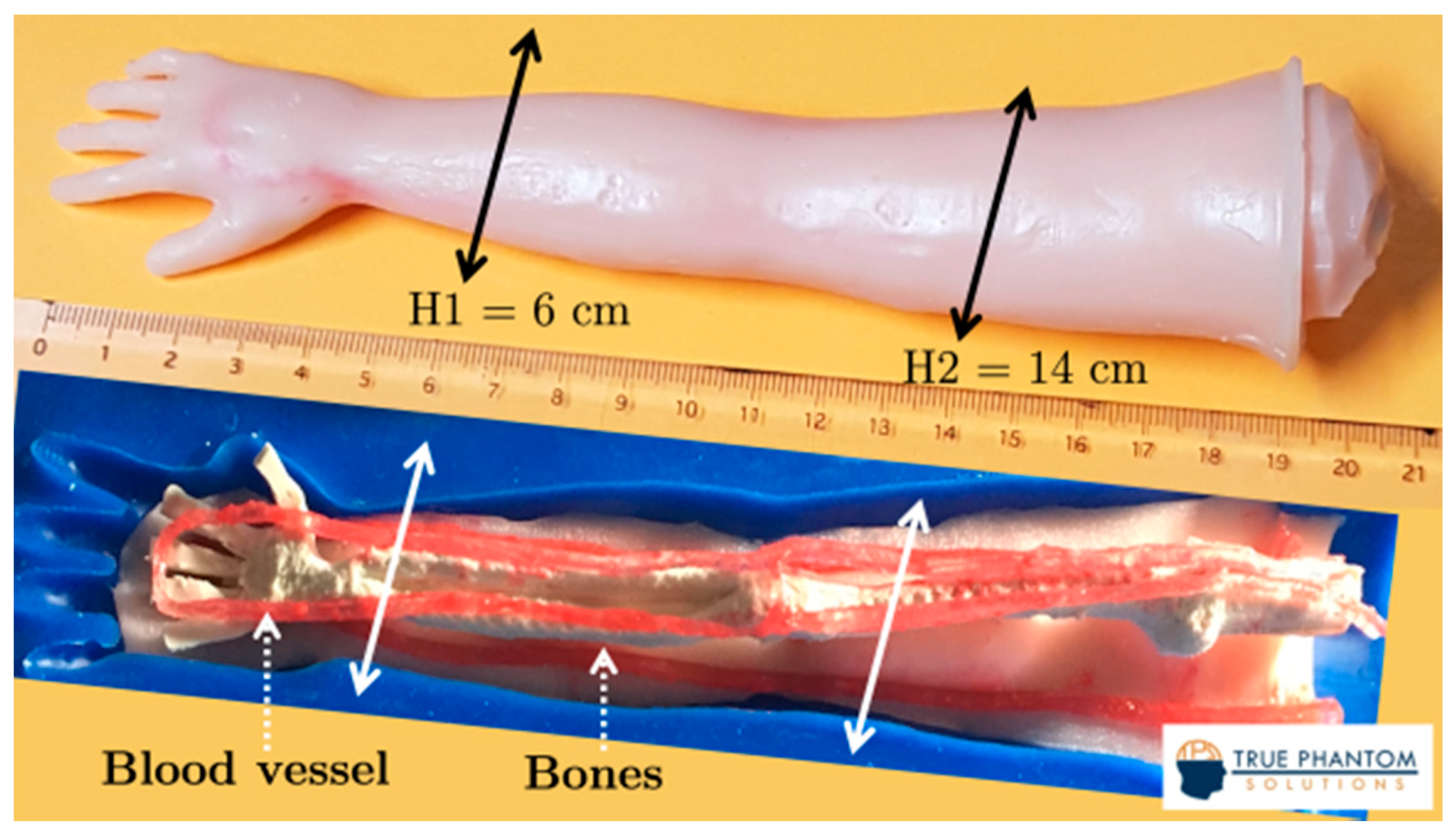
3.1. Samples
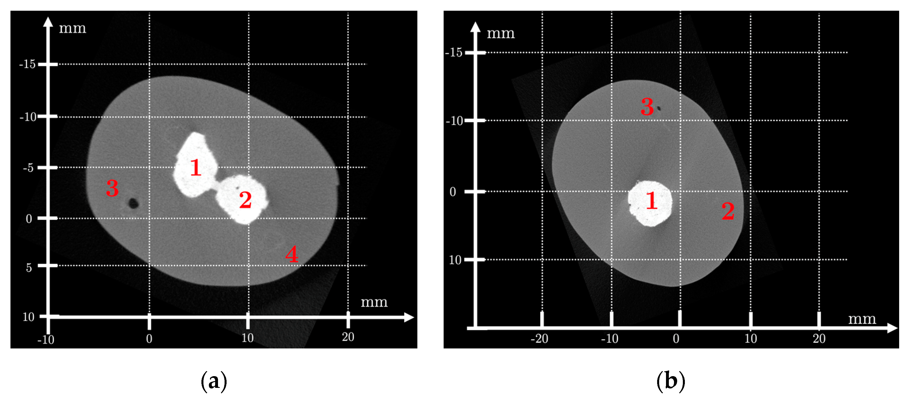
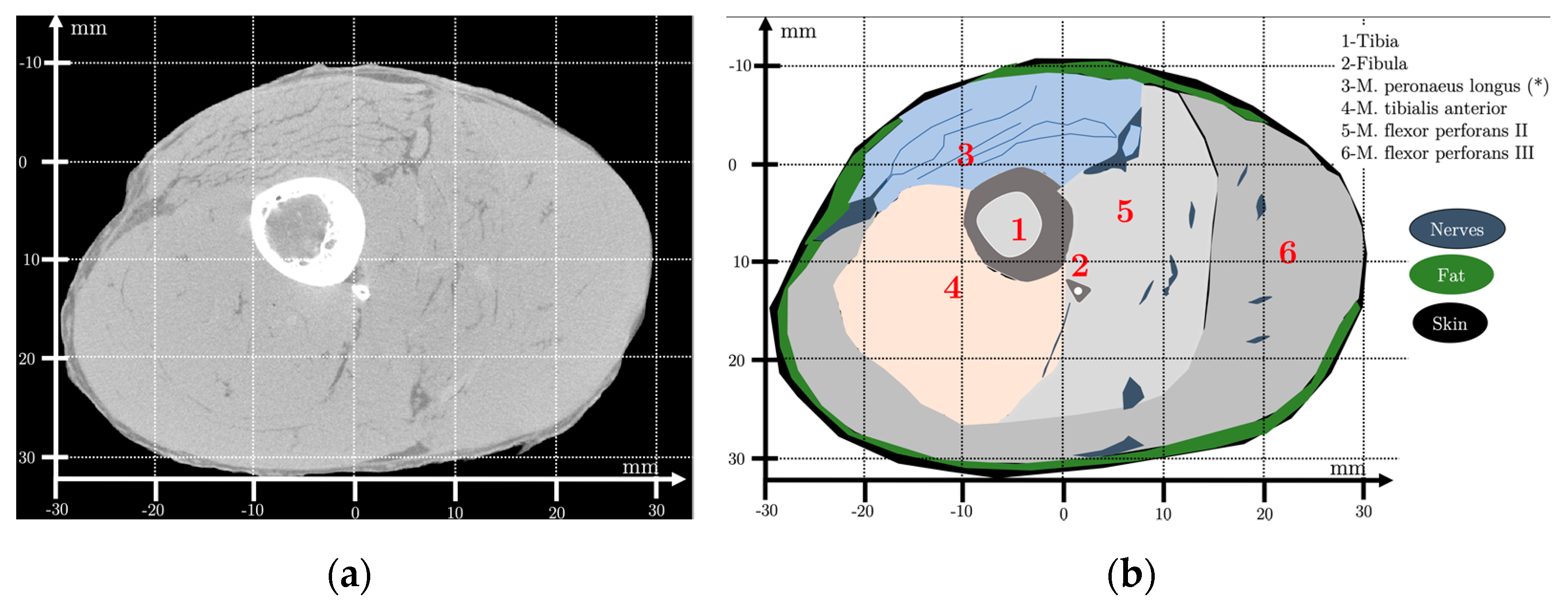
3.2. X-ray μCT
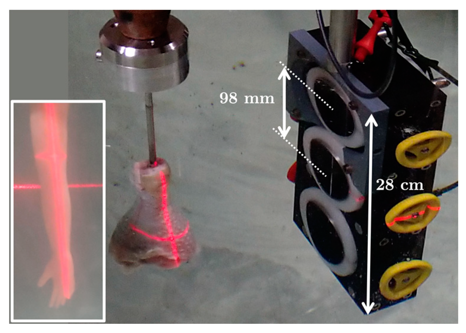
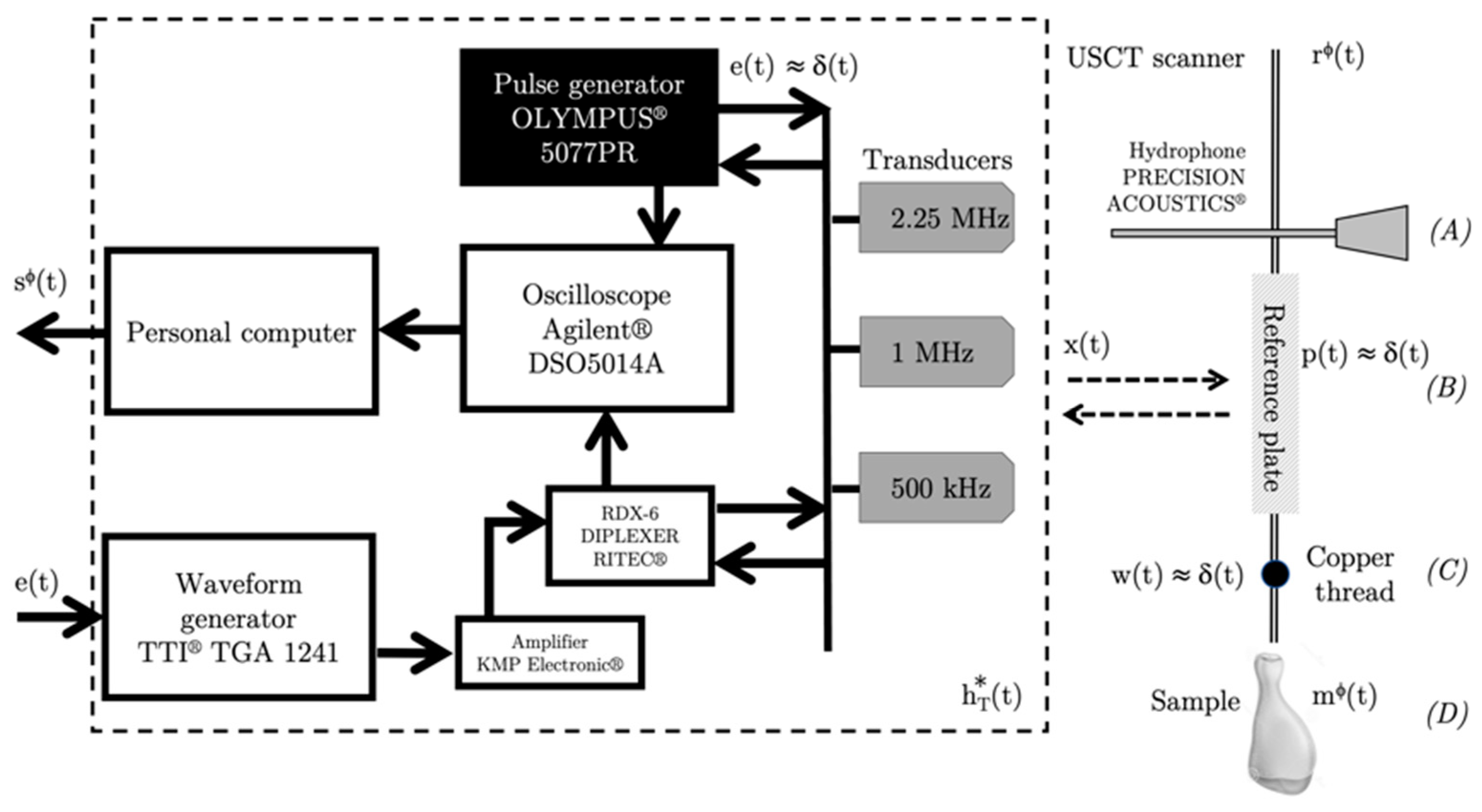
3.3. USCT Scanner
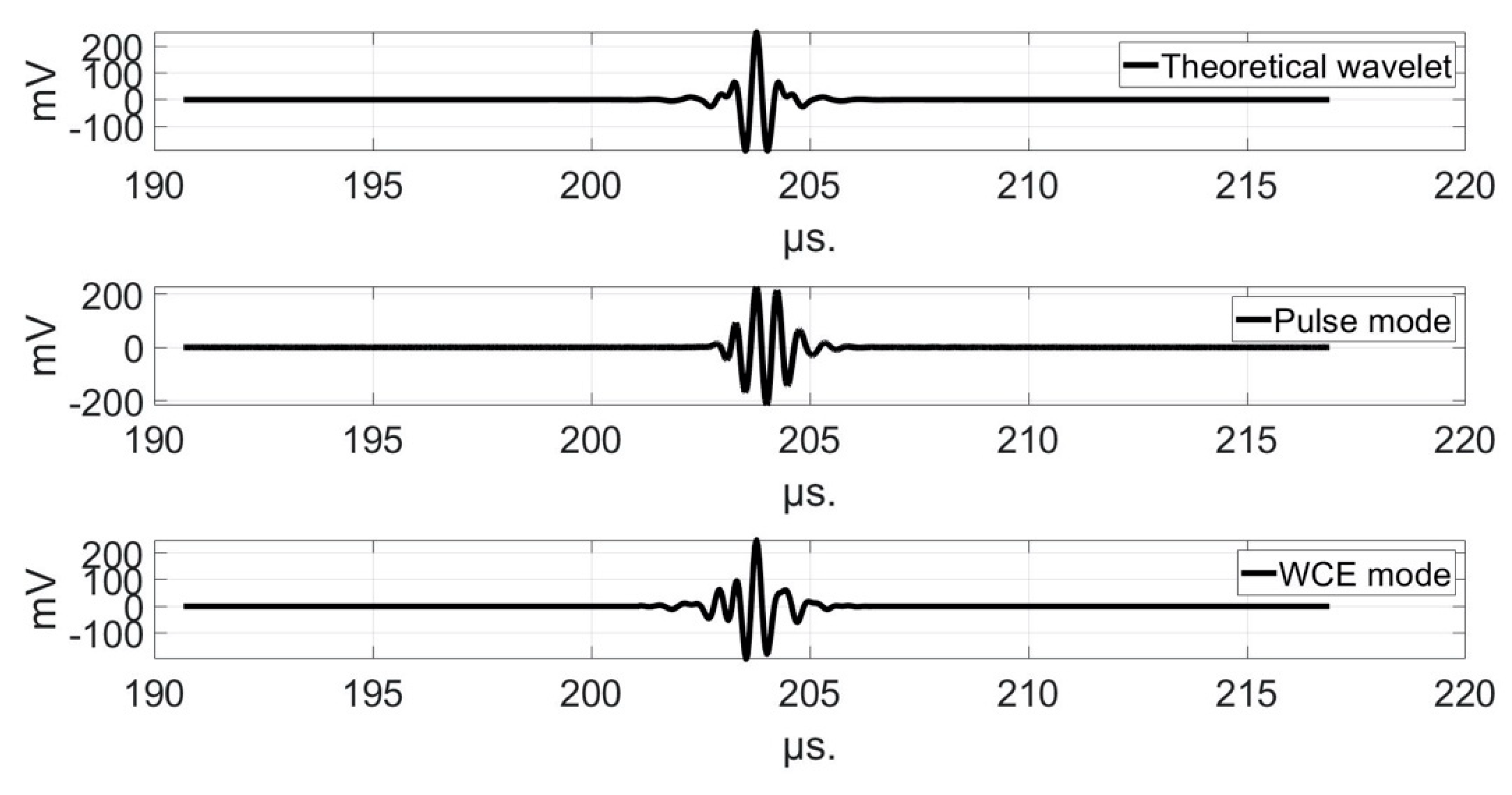
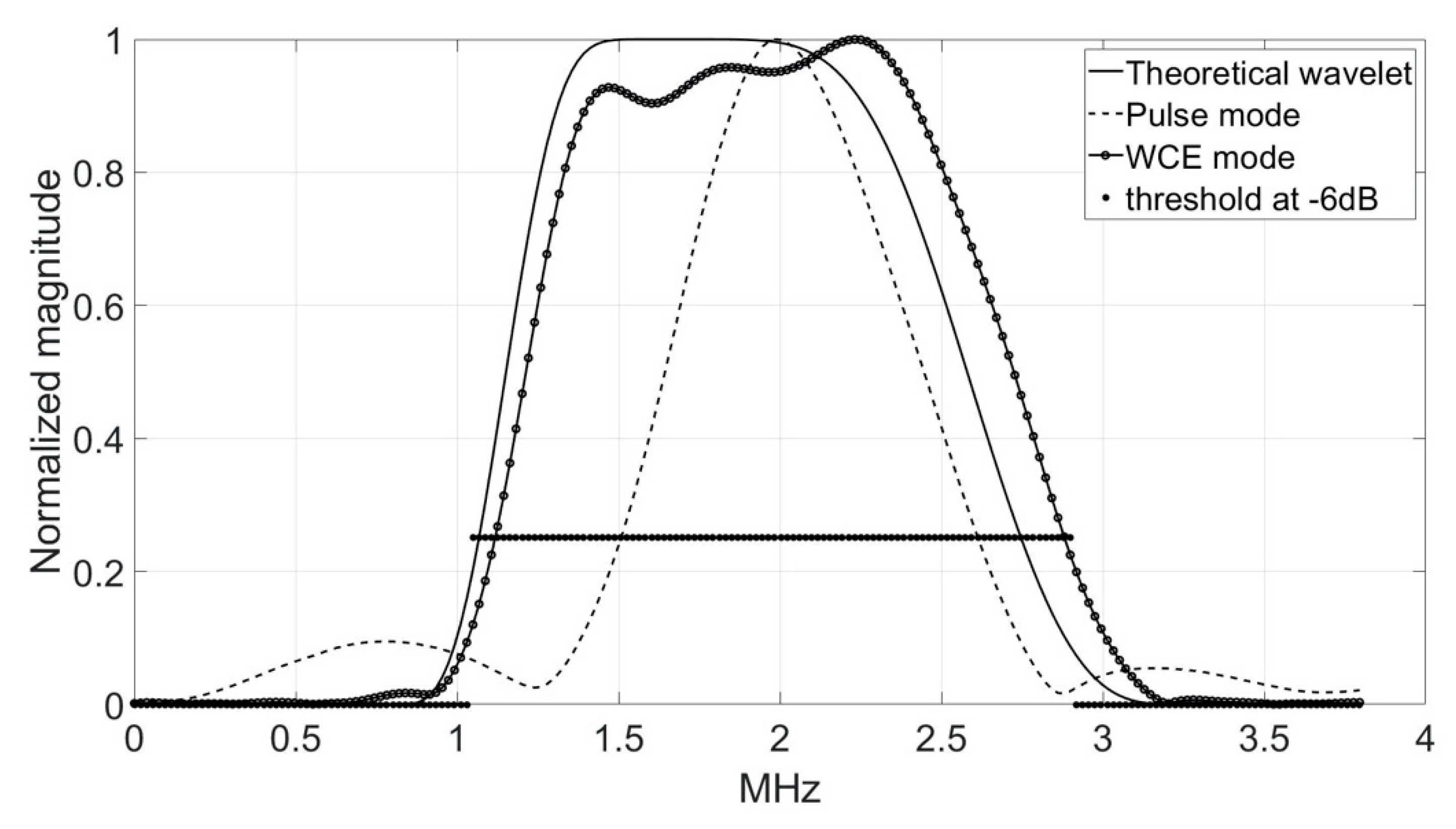
3.4. Transducers and Electro-Acoustic Devices
3.5. Experimental Conditions
3.6. Transmitted and Received Signals
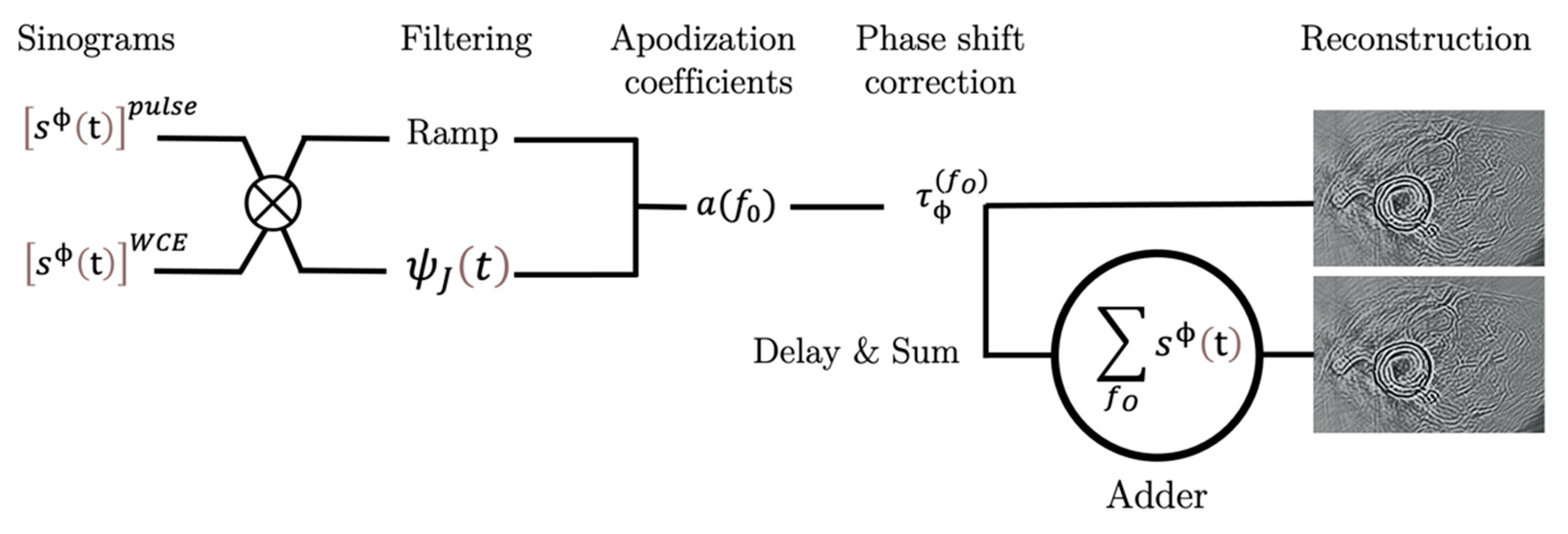
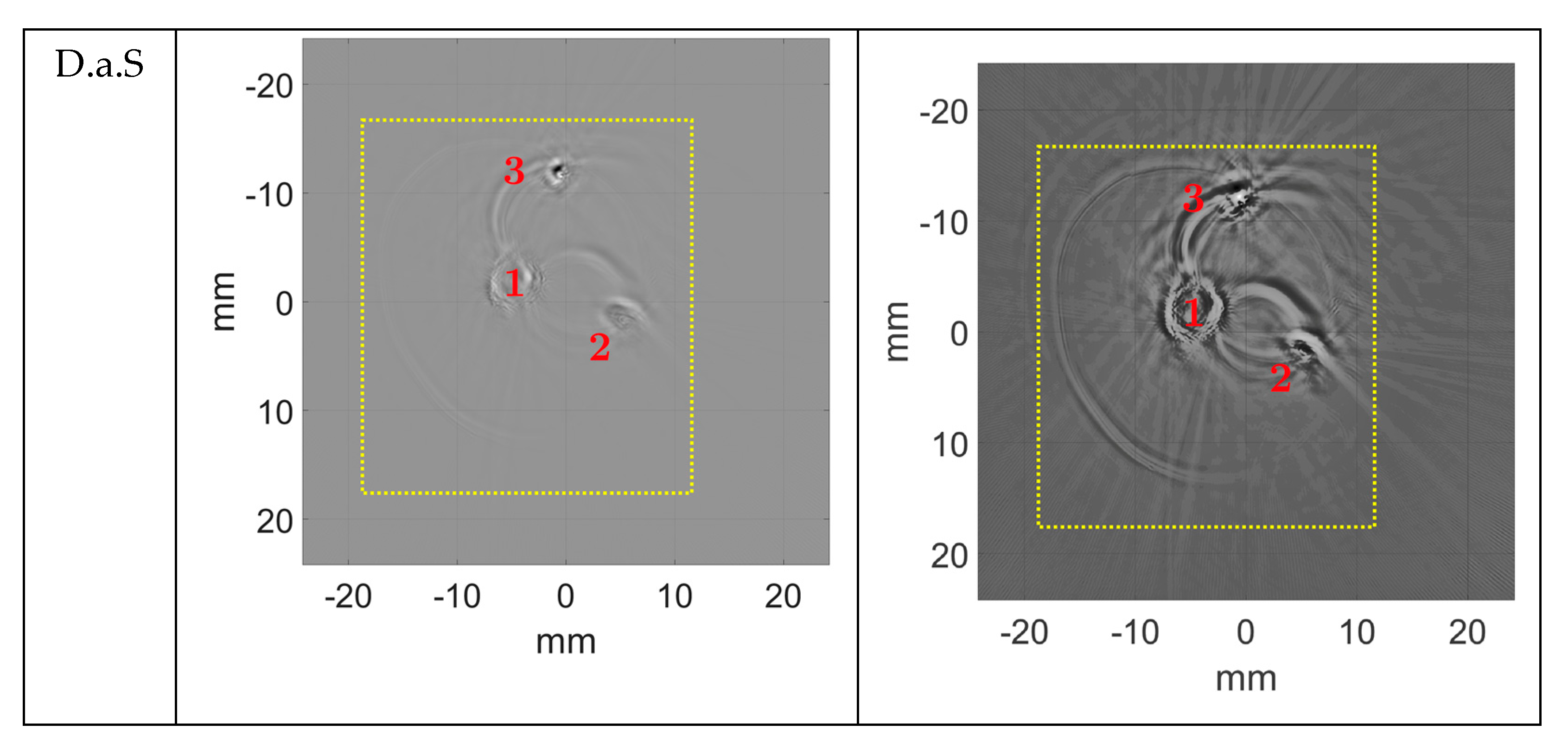
3.7. Delay-and-Sum Processing (D.a.S.)
3.8. Acoustical Intensities
4. Results
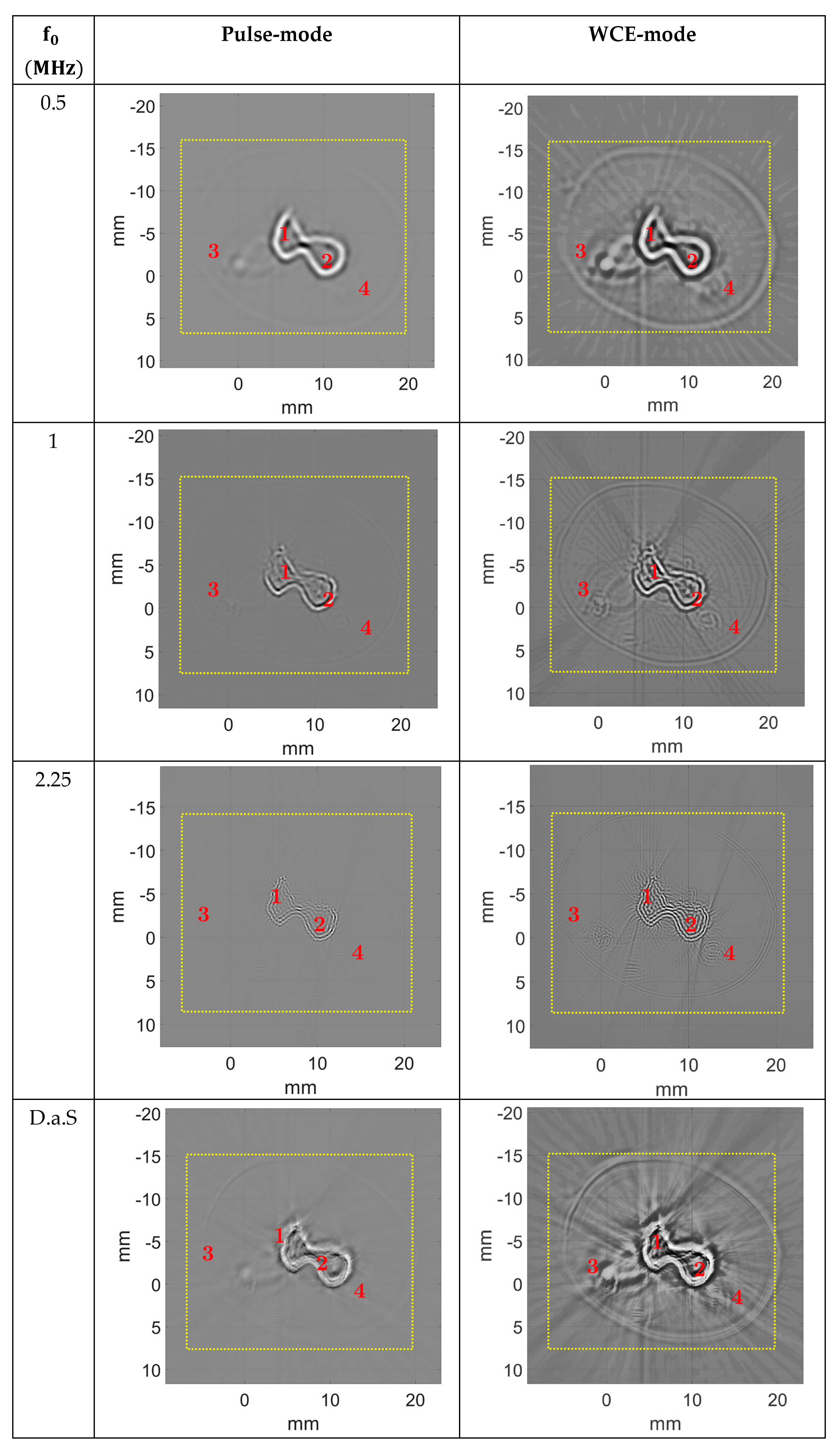
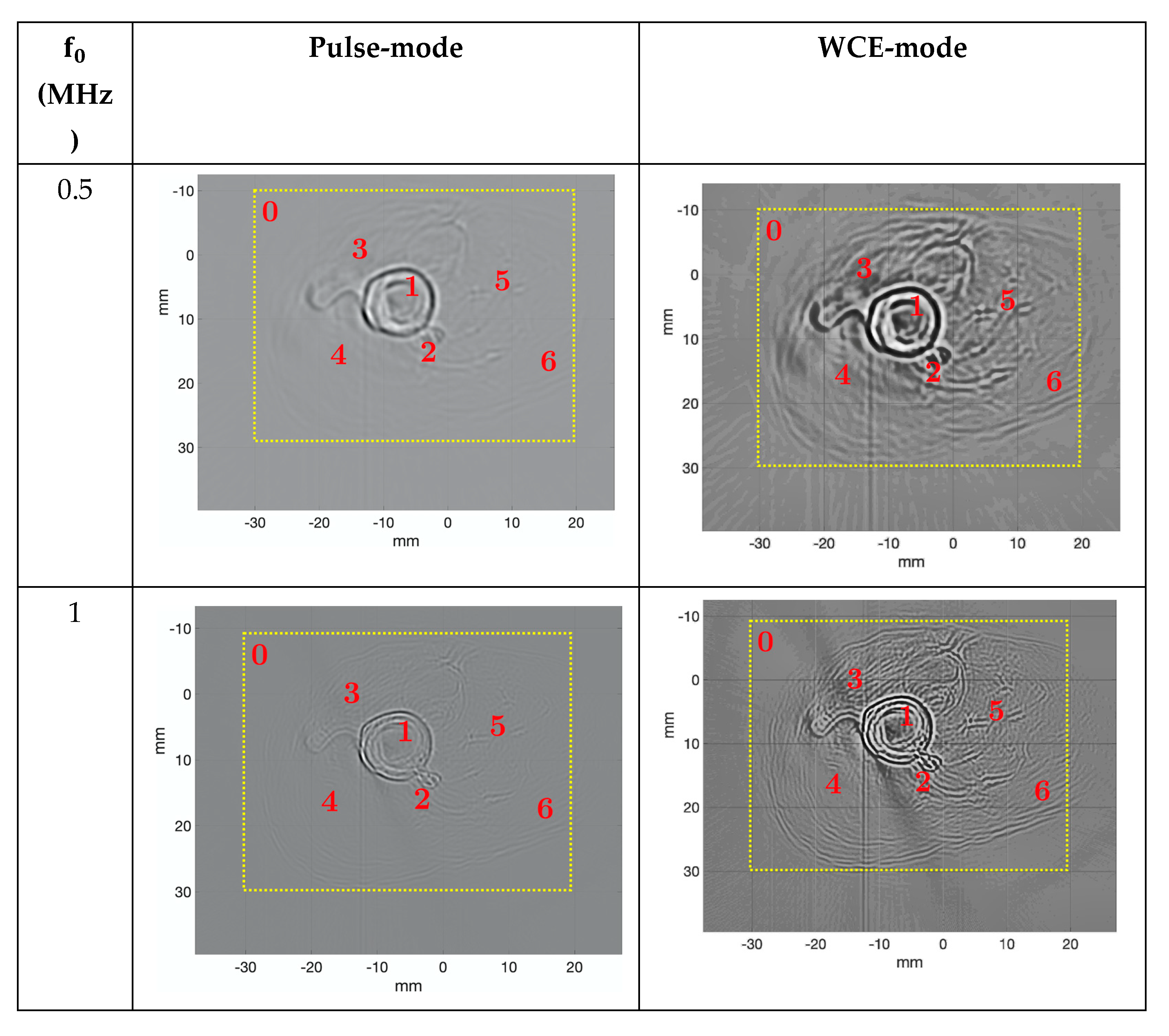
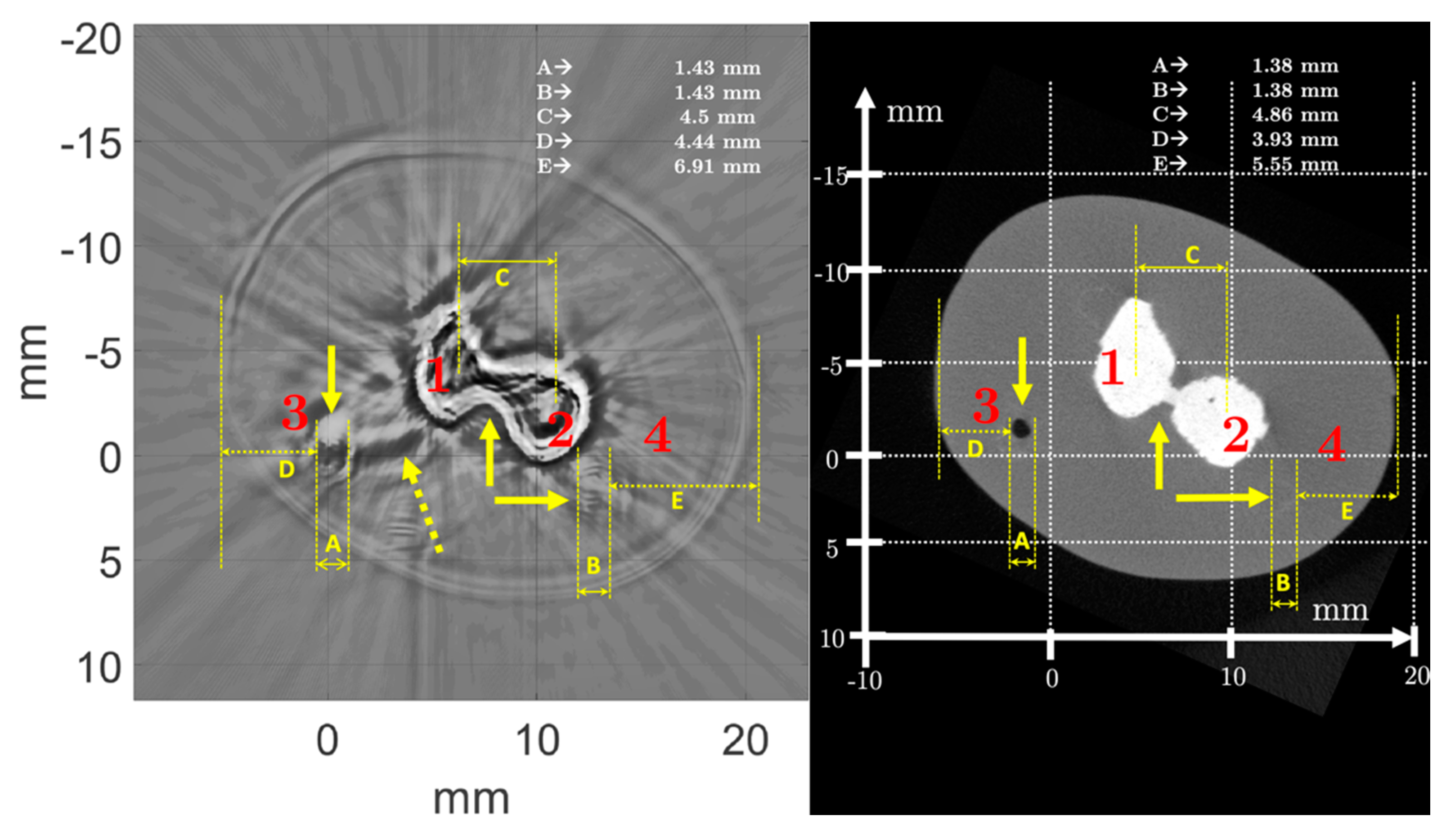
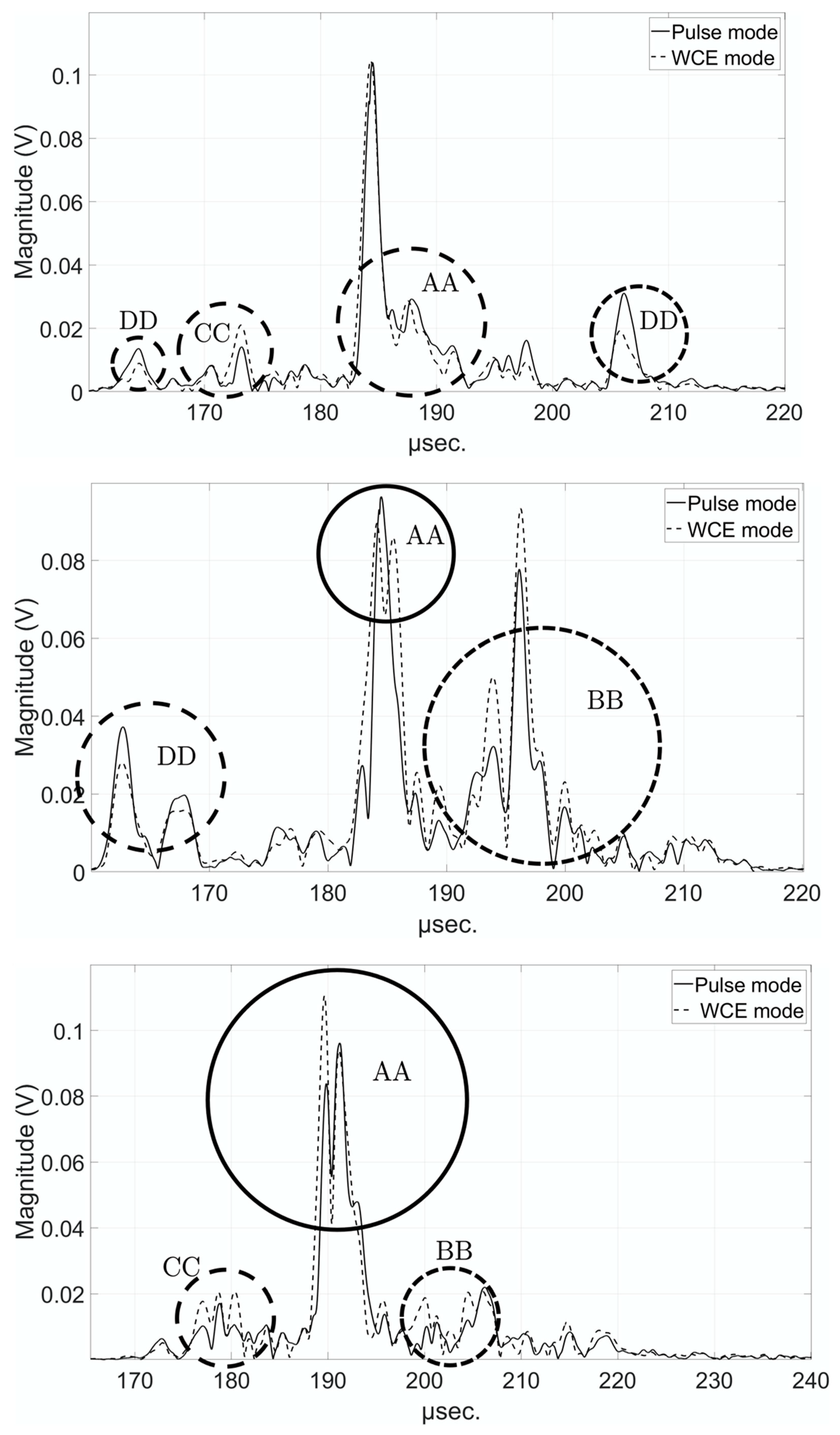
4.1. Comparison of Pulse and WCE-Mode Methods for the Newborn Arm Phantom
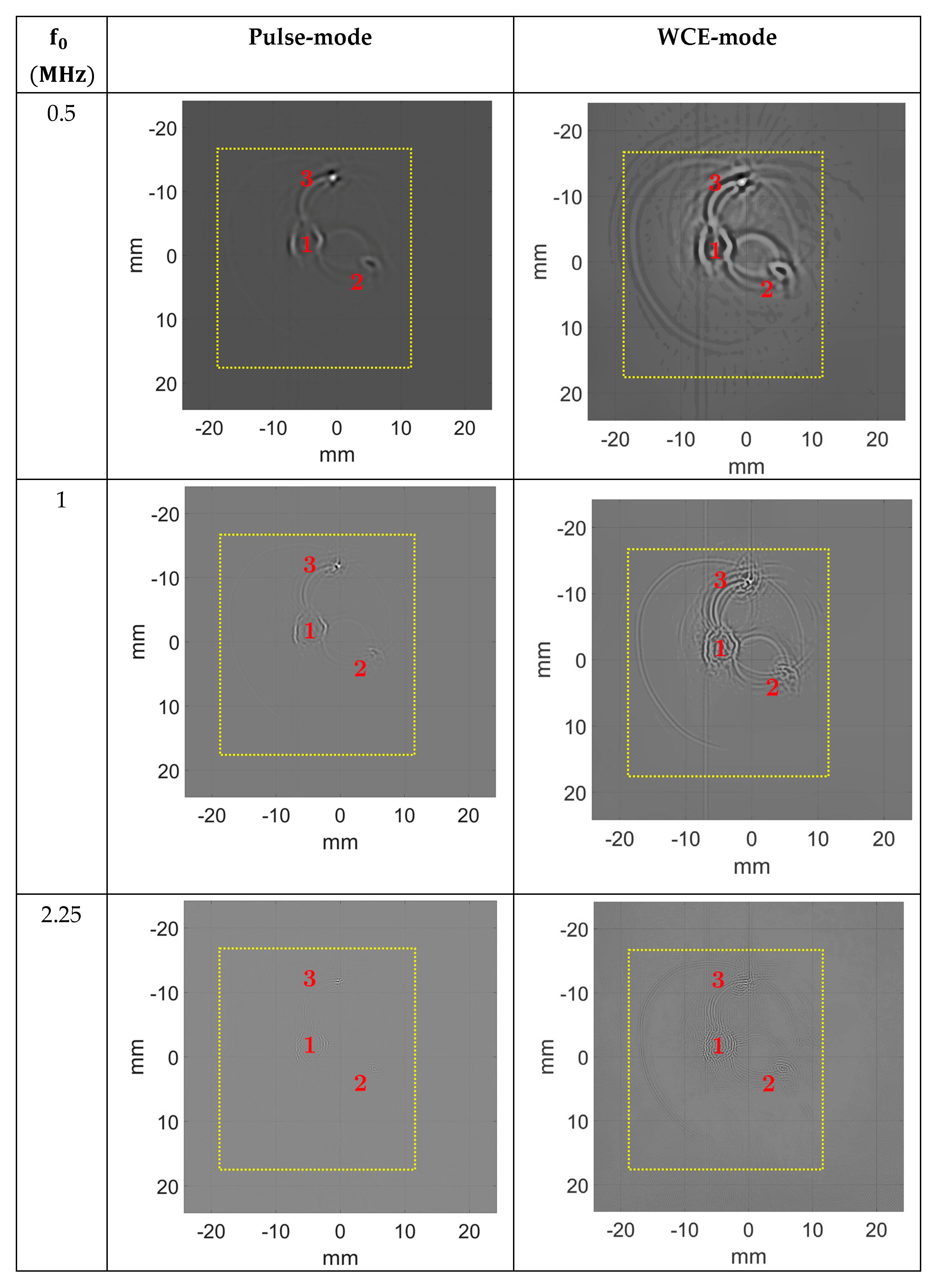
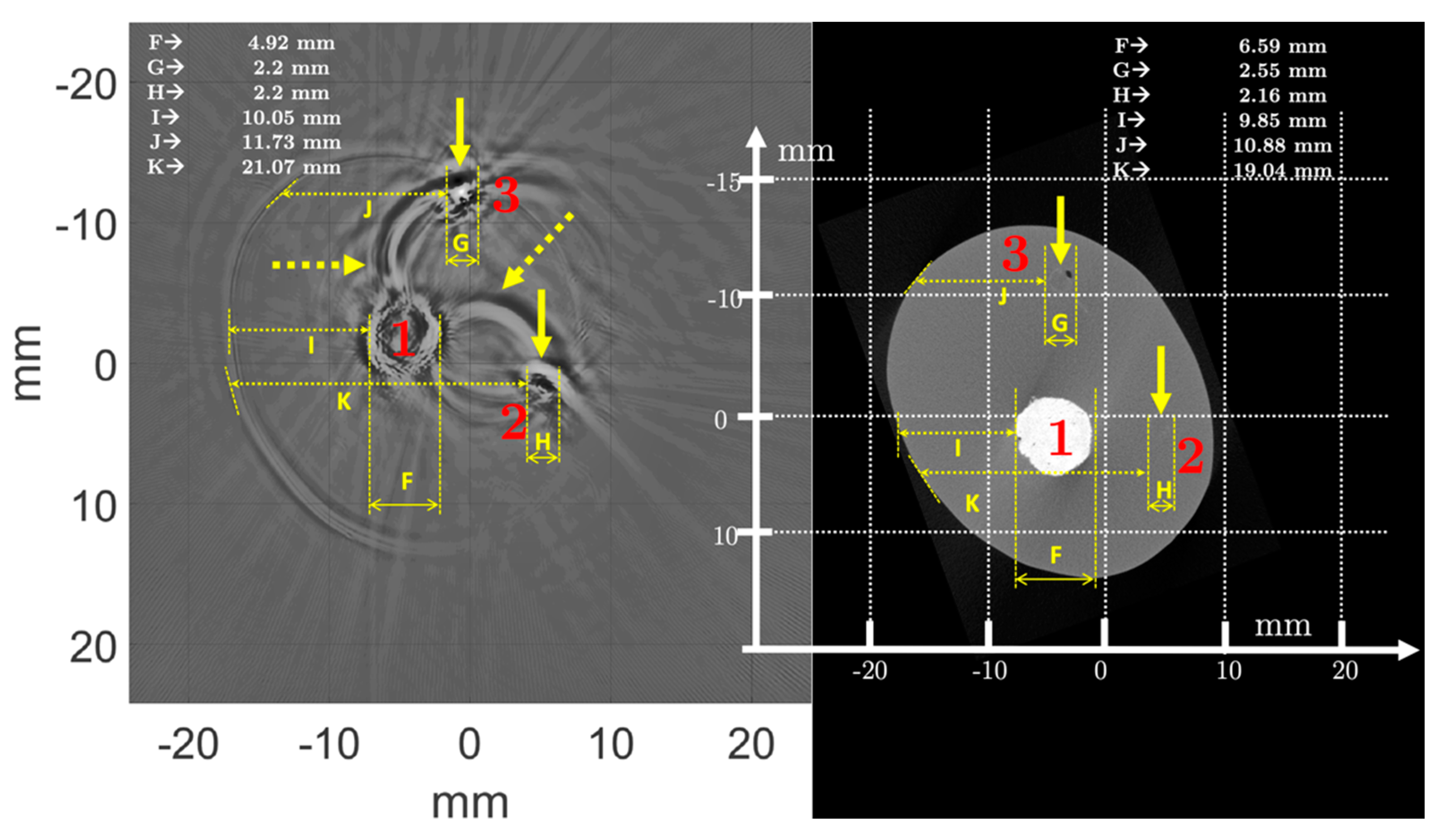
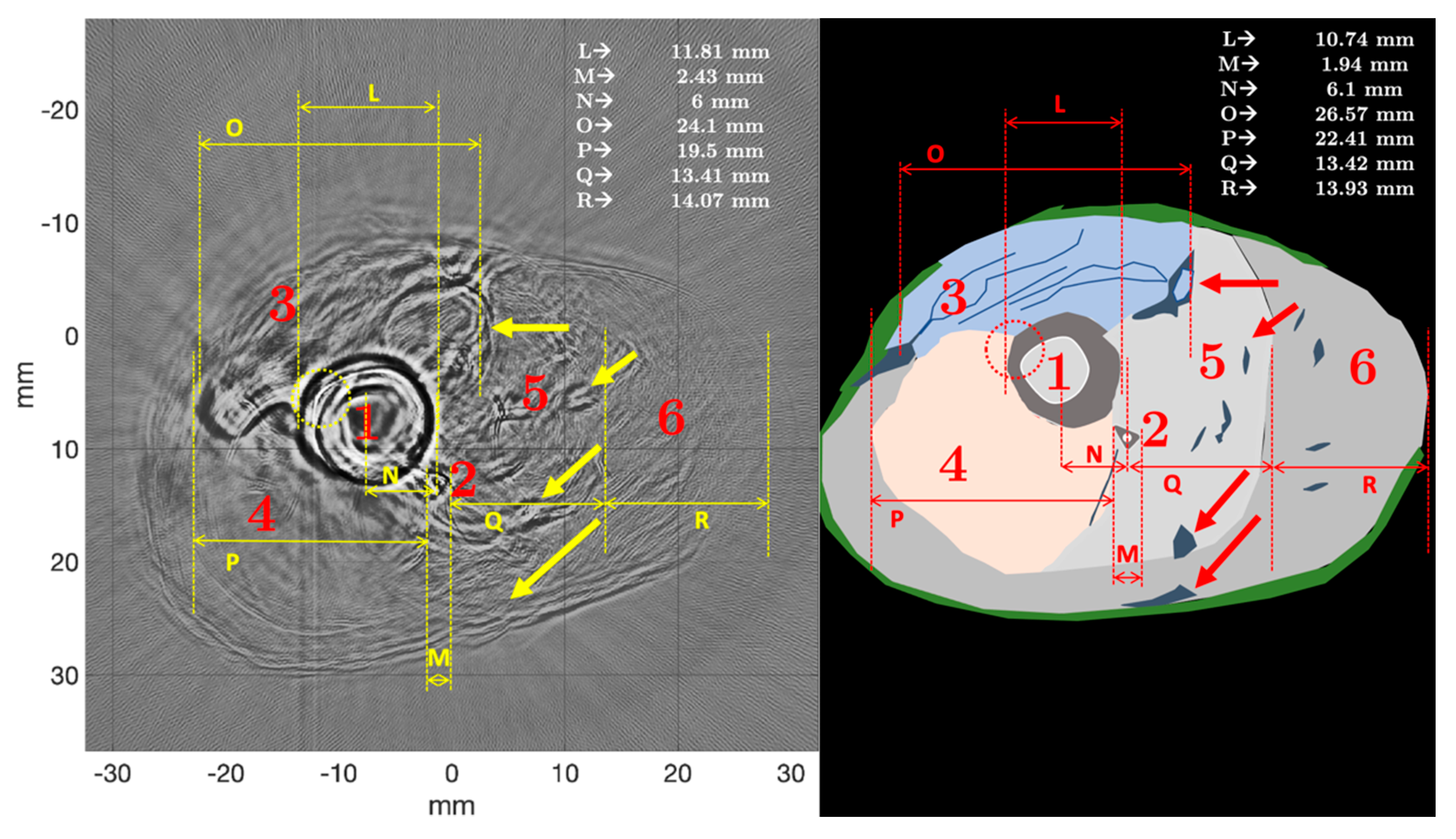
4.2. Comparison of Pulse- and WCE-Mode Methods for the Ex Vivo Chicken Drumstick
4.3. Study of the Contrast-to-Noise Ratio
5. Discussions
5.1. Anatomy and Morphometry
5.2. Pulse-Mode USCT versus WCE-Mode USCT
5.3. Intensity, Ultrasonic Field, and Beam Aperture
5.4. Usefulness on Living Tissue
6. Conclusions
Author Contributions
Funding
Institutional Review Board Statement
Acknowledgments
Conflicts of Interest
References
- Griffith, J.F. Diagnostic Ultrasound: Musculoskeletal, 2nd ed.; Amirsys Publishing: Salt Lake City, UT, USA, 2019; ISBN 978-1-937242-17-6. [Google Scholar]
- Riccabona, M. (Ed.) Pediatric Ultrasound: Requisites and Applications, 2nd ed.; Springer: Cham, Switzerland, 2020; ISBN 978-3-030-47909-1. [Google Scholar]
- Aldrich, J.E. Basic physics of ultrasound imaging. Crit. Care Med. 2007, 35, S131–S137. [Google Scholar] [CrossRef] [PubMed]
- André, M.P.; Martin, P.J.; Otto, G.P.; Olson, L.K.; Barrett, T.K.; Spivey, B.A.; Palmer, D.A. A New Consideration of Diffraction Computed Tomography for Breast Imaging: Studies in Phantoms and Patients. In Acoustical Imaging; Jones, J.P., Ed.; Springer: Boston, MA, USA, 1995; pp. 379–390. ISBN 978-1-4615-1943-0. [Google Scholar]
- Mensah, S.; Ferriere, R. Diffraction tomography: A geometrical distortion free procedure. Ultrasonics 2004, 42, 677–682. [Google Scholar] [CrossRef] [PubMed]
- Lefebvre, J.-P.; Lasaygues, P.; Mensah, S. Acoustic Tomography, Ultrasonic Tomography. In Materials and Acoustics Handbook; Bruneau, M., Potel, C., Eds.; ISTE: London, UK, 2009; pp. 887–906. ISBN 978-0-470-61160-9. [Google Scholar]
- Hopp, T.; Ruiter, N.; Bamber, J.C.; Duric, N.; Van Dongen, K.W.A. Proceedings of the International Workshop on Medical Ultrasound Tomography, Speyer, Germany, 1–3 November 2017; KIT Scientific Publishing: Karlruhe, Germany, 2017. [Google Scholar]
- Lasaygues, P.; Guillermin, R.; Lefebvre, J.P. Ultrasonic Computed Tomography. In Bone Quantitative Ultrasound; Springer: Berlin/Heidelberg, Germany, 2011; pp. 441–459. [Google Scholar]
- Wang, K.; Matthews, T.; Anis, F.; Li, C.; Duric, N.; Anastasio, M.A. Breast Ultrasound Computed Tomography Using Waveform Inversion with Source Encoding. In Proceedings of the Medical Imaging 2015: Ultrasonic Imaging and Tomography; Bosch, J.G., Duric, N., Eds.; SPIE: Orlando, FL, USA, 2015; p. 94190C. [Google Scholar]
- Sandhu, G.Y.; Li, C.; Roy, O.; Schmidt, S.; Duric, N. Frequency domain ultrasound waveform tomography: Breast imaging using a ring transducer. Phys. Med. Biol. 2015, 60, 5381–5398. [Google Scholar] [CrossRef] [PubMed]
- Bernard, S.; Monteiller, V.; Komatitsch, D.; Lasaygues, P. Ultrasonic computed tomography based on full-waveform inversion for bone quantitative imaging. Phys. Med. Biol. 2017, 62, 7011–7035. [Google Scholar] [CrossRef] [PubMed]
- Pérez-Liva, M.; Herraiz, J.L.; Udías, J.M.; Miller, E.; Cox, B.T.; Treeby, B.E. Time domain reconstruction of sound speed and attenuation in ultrasound computed tomography using full wave inversiona. J. Acoust. Soc. Am. 2017, 141, 1595–1604. [Google Scholar] [CrossRef] [PubMed]
- Calderon Agudo, O.; Guasch, L.; Huthwaite, P.; Warner, M. 3D Imaging of the Breast Using Full-Waveform Inversion; Bamber, J., van Dongen, K.W.A., Duric, N., Hopp, T., Ruiter, N.V., Eds.; KIT Scientific Publishing: Karlruhe, Germany, 2017; pp. 99–110. [Google Scholar]
- Falardeau, T.; Belanger, P. Ultrasound tomography in bone mimicking phantoms: Simulations and experiments. J. Acoust. Soc. Am. 2018, 144, 2937–2946. [Google Scholar] [CrossRef] [PubMed]
- Wiskin, J.W.; Malik, B.; Natesan, R.; Pirshafiey, N.; Klock, J.; Lenox, M. 3D full inverse scattering ultrasound tomography of the human knee (Conference Presentation). In Proceedings of the Medical Imaging 2019: Ultrasonic Imaging and Tomography; Ruiter, N.V., Byram, B.C., Eds.; SPIE: San Diego, CA, USA, 2019; p. 25. [Google Scholar]
- Wiskin, J.; Malik, B.; Borup, D.; Pirshafiey, N.; Klock, J. Full wave 3D inverse scattering transmission ultrasound tomography in the presence of high contrast. Sci. Rep. 2020, 10, 20166. [Google Scholar] [CrossRef] [PubMed]
- Guasch, L.; Calderón Agudo, O.; Tang, M.-X.; Nachev, P.; Warner, M. Full-waveform inversion imaging of the human brain. NPJ Digit. Med. 2020, 3, 28. [Google Scholar] [CrossRef] [PubMed]
- Espinosa, L.; Doveri, E.; Bernard, S.; Monteiller, V.; Guillermin, R.; Lasaygues, P. Ultrasonic Imaging of High-contrasted Objects Based on Full-waveform Inversion: Limits under Fluid Modeling. Ultrason. Imaging 2021, 43, 88–99. [Google Scholar] [CrossRef] [PubMed]
- Lefebvre, J.-P. Progress in linear inverse scattering imaging: NDE application of Ultrasonic Reflection Tomography. In Inverse Problem in Engineering Mechanics; Balkema, A.A., Ed.; Brookfield: Rotterdam, The Netherlands, 1994; pp. 371–375. [Google Scholar]
- Zheng, R.; Lasaygues, P. Simultaneous Assessment of Bone Thickness and Velocity for Ultrasonic Computed Tomography Using Transmission-Echo Method. In Proceedings of the 2013 IEEE International Ultrasonics Symposium (IUS), Prague, Czech Republic, 21–25 July 2013; pp. 2084–2087. [Google Scholar]
- Shortell, M.P.; Althomali, M.A.M.; Wille, M.-L.; Langton, C.M. Combining Ultrasound Pulse-Echo and Transmission Computed Tomography for Quantitative Imaging the Cortical Shell of Long-Bone Replicas. Front. Mater. 2017, 4, 40. [Google Scholar] [CrossRef]
- Lasaygues, P. Assessing the cortical thickness of long bone shafts in children, using two-dimensional ultrasonic diffraction tomography. Ultrasound Med. Biol. 2006, 32, 1215–1227. [Google Scholar] [CrossRef] [PubMed][Green Version]
- Duric, N.; Littrup, P.; Poulo, L.; Babkin, A.; Pevzner, R.; Holsapple, E.; Rama, O.; Glide, C. Detection of breast cancer with ultrasound tomography: First results with the Computed Ultrasound Risk Evaluation (CURE) prototype: Detection of breast cancer with ultrasound tomography. Med. Phys. 2007, 34, 773–785. [Google Scholar] [CrossRef] [PubMed]
- Rouyer, J.; Mensah, S.; Vasseur, C.; Lasaygues, P. The benefits of compression methods in acoustic coherence tomography. Ultrason. Imaging 2015, 37, 205–223. [Google Scholar] [CrossRef] [PubMed]
- Lasaygues, P.; Arciniegas, A.; Espinosa, L.; Prieto, F.; Brancheriau, L. Accuracy of coded excitation methods for measuring the time of flight: Application to ultrasonic characterization of wood samples. Ultrasonics 2018, 89, 178–186. [Google Scholar] [CrossRef] [PubMed]
- Loosvelt, M.; Lasaygues, P. A Wavelet-Based Processing method for simultaneously determining ultrasonic velocity and material thickness. Ultrasonics 2011, 51, 325–339. [Google Scholar] [CrossRef] [PubMed]
- Metwally, K.; Lefevre, E.; Baron, C.; Zheng, R.; Pithioux, M.; Lasaygues, P. Measuring mass density and ultrasonic wave velocity: A wavelet-based method applied in ultrasonic reflection mode. Ultrasonics 2016, 65, 10–17. [Google Scholar] [CrossRef] [PubMed]
- Lasaygues, P.; Guillermin, R.; Metwally, K.; Fernandez, S.; Balasse, L.; Petit, P.; Baron, C. Contrast resolution enhancement of Ultrasonic Computed Tomography using a wavelet-based method—Preliminary results in bone imaging. In Proceedings of the International Workshop on Medical Ultrasound Tomography; Bamber, J., van Dongen, K.W.A., Duric, N., Hopp, T., Ruiter, N.V., Eds.; KIT Scientific Publishing: Karlruhe, Germany, 2017; pp. 291–302. [Google Scholar]
- Retz, K.; Kotopoulis, S.; Kiserud, T.; Matre, K.; Eide, G.E.; Sande, R. Measured acoustic intensities for clinical diagnostic ultrasound transducers and correlation with thermal index: Acoustic intensity and TI. Ultrasound Obstet. Gynecol. 2017, 50, 236–241. [Google Scholar] [CrossRef] [PubMed]
- Preston, R.C. Output Measurements for Medical Ultrasound.; Springer: London, UK, 1991; ISBN 978-1-4471-1883-1. [Google Scholar]
- Kak, A.; Slaney, M. Principles of Computerized Tomographic Imaging; Society for Industrial and Applied Mathematics: Philadelphia, PA, USA, 2001. [Google Scholar]
- Deans, S.R. The Radon Transform and some of Its Applications; Dover Publications: Mineola, NY, USA, 2007; ISBN 978-0-486-46241-7. [Google Scholar]
- Devaney, A.J. Mathematical Foundations of Imaging, Tomography and Wavefield Inversion; Cambridge University Press: Cambridge, MA, USA, 2012; ISBN 978-0-521-11974-0. [Google Scholar]
- Holschneider, M. Inverse Radon transforms through inverse wavelet transforms. Inverse Probl. 1991, 7, 853–861. [Google Scholar] [CrossRef]
- Jaffard, S. Construction of Wavelets on Open Sets. In Wavelets; Combes, J.-M., Grossmann, A., Tchamitchian, P., Eds.; Springer: Berlin/Heidelberg, Germany, 1989; pp. 247–252. ISBN 978-3-642-97179-2. [Google Scholar]
- Jaffard, S.; Meyer, Y.; Ryan, R.D. Wavelets: Tools for Science and Technology; Society for Industrial and Applied Mathematics: Philadelphia, PA, USA, 2001; ISBN 978-0-89871-448-7. [Google Scholar]
- Meyer, Y. Orthonormal Wavelets. In Wavelets; Combes, J.-M., Grossmann, A., Tchamitchian, P., Eds.; Springer: Berlin/Heidelberg, Germany, 1989; pp. 21–37. ISBN 978-3-642-97179-2. [Google Scholar]
- Schindelin, J.; Arganda-Carreras, I.; Frise, E.; Kaynig, V.; Longair, M.; Pietzsch, T.; Preibisch, S.; Rueden, C.; Saalfeld, S.; Schmid, B.; et al. Fiji: An open-source platform for biological-image analysis. Nat. Methods 2012, 9, 676–682. [Google Scholar] [CrossRef]
- National Council on Radiation Protection and Measurements (Ed.) Biological Effects of Ultrasound: Mechanisms and Clinical Implications; NCRP report; The Council: Bethesda, MD, USA, 1983; ISBN 978-0-913392-64-5. [Google Scholar]
- Renaud, G.; Kruizinga, P.; Cassereau, D.; Laugier, P. In vivo ultrasound imaging of the bone cortex. Phys. Med. Biol. 2018, 63, 125010. [Google Scholar] [CrossRef] [PubMed]


| Type of Tissue | Ultrasonic Velocity (m/s) | Mass Density (g/cm3) | Impedance (MRays) | Attenuation (dB/cm) |
|---|---|---|---|---|
| Soft body | 1423 ± 10 | 1.0 | ≈1.423 | 1.1 ± 0.2 |
| Blood vessel | 1400 ± 10 | 1.02 | ≈1.428 | 1.7 ± 0.2 |
| Bone | 1129 ± 5 | 2.16 | ≈0.0024 | 21 ± 2.0 |
| Parameter (−6 dB) | 500 kHz | 1 MHz | 2.25 MHz |
|---|---|---|---|
| Nominal frequency | 477 kHz | 858 kHz | 2 MHz |
| Broadband width | 591 kHz | 900 kHz | 1 MHz |
| Bandwidth | (229–820) kHz | (0.5–1.3) MHz | (1.5–2.6) MHz |
| AUC (normalized) | 0.394 | 0.459 | 0.76 |
| Pulse duration () | 1.7 μs | 1.2 μs | 1 μs |
| Axial resolution | 2.5 mm | 1.8 mm | 1.5 mm |
| Theoretical Parameter | 500 kHz | 1 MHz | 2.25 MHz |
| −9 | −8 | −7 | |
| Center frequency () | 651 kHz | 1.3 MHz | 2.6 MHz |
| Bandwidth | (0.325–1.3) MHz | (0.651–2.6) MHz | (1.3–5.2) MHz |
| −6 dB Parameters | |||
| Broadband width | 458 kHz | 900 kHz | 1.66 MHz |
| Bandwidth | (248–706) kHz | (0.5–1.4) MHz | (1.04–2.7) MHz |
| AUC (normalized) | 0.349 | 0.694 | 1.38 |
| Pulse duration () | 2.2 μs | 0.74 μs | 0.5 μs |
| Axial resolution | 3.2 mm | 1.1 mm | 743 μm |
| Parameter (−6 dB) | 500 kHz | 1 MHz | 2.25 MHz |
|---|---|---|---|
| Nominal frequency | 553 kHz | 744 kHz | 2.23 MHz |
| Broadband width | 458 kHz | 900 kHz | 1.8 MHz |
| Bandwidth | (267–725) kHz | (0.5–1.4) MHz | (1.1–2.9) MHz |
| AUC (normalized) | 0.347 | 0.655 | 1.42 |
| Pulse duration () | 2.2 μs | 1.2 μs | 0.56 μs |
| Axial resolution | 3.2 mm | 1.8 mm | 832 μm |
| 500 kHz | 641 | −641 | 27.6 | 0.93 |
| 1 MHz | 529.5 | −517.4 | 18.8 | 0.56 |
| 2.25 MHz | 540.8 | −540.8 | 19.6 | 0.38 |
| Pulse-Mode | WCE-Mode | Gain (%) | |
|---|---|---|---|
| Newborn arm phantom (H1) | |||
| 0.5 | 0.11 (0.1) | 1.6 (1.3) | 1355 |
| 1 | 0.083 (0.076) | 0.62 (0.54) | 647 |
| 2.25 | 1 (1) | 3.9 (5.6) | 290 |
| D.a.S | 0.16 (0.16) | 0.89 (0.75) | 456 |
| Newborn arm phantom (H2) | |||
| 0.5 | 0.13 (0.1) | 3.5 (2.6) | 2592 |
| 1 | 0.069 (0.058) | 1.3 (1.1) | 1784 |
| 2.25 | 0.11 (0.093) | 1.5 (0.64) | 1264 |
| D.a.S | 0.12 (0.11) | 2 (0.99) | 1567 |
| Ex vivo chicken drumstick | |||
| 0.5 | 0.3 (0.23) | 2.1 (1.4) | 600 |
| 1 | 0.41 (0.31) | 1.1 (1) | 175 |
| 2.25 | 0.19 (0.11) | 0.37 (0.19) | 95 |
| D.a.S | 0.22 (0.18) | 0.46 (0.26) | 109 |
Publisher’s Note: MDPI stays neutral with regard to jurisdictional claims in published maps and institutional affiliations. |
© 2021 by the authors. Licensee MDPI, Basel, Switzerland. This article is an open access article distributed under the terms and conditions of the Creative Commons Attribution (CC BY) license (https://creativecommons.org/licenses/by/4.0/).
Share and Cite
Doveri, E.; Sabatier, L.; Long, V.; Lasaygues, P. Reflection-Mode Ultrasound Computed Tomography Based on Wavelet Processing for High-Contrast Anatomical and Morphometric Imaging. Appl. Sci. 2021, 11, 9368. https://doi.org/10.3390/app11209368
Doveri E, Sabatier L, Long V, Lasaygues P. Reflection-Mode Ultrasound Computed Tomography Based on Wavelet Processing for High-Contrast Anatomical and Morphometric Imaging. Applied Sciences. 2021; 11(20):9368. https://doi.org/10.3390/app11209368
Chicago/Turabian StyleDoveri, Elise, Laurent Sabatier, Vincent Long, and Philippe Lasaygues. 2021. "Reflection-Mode Ultrasound Computed Tomography Based on Wavelet Processing for High-Contrast Anatomical and Morphometric Imaging" Applied Sciences 11, no. 20: 9368. https://doi.org/10.3390/app11209368
APA StyleDoveri, E., Sabatier, L., Long, V., & Lasaygues, P. (2021). Reflection-Mode Ultrasound Computed Tomography Based on Wavelet Processing for High-Contrast Anatomical and Morphometric Imaging. Applied Sciences, 11(20), 9368. https://doi.org/10.3390/app11209368