Effects of Phase Shift Errors in Recurrence Plot for Rotating Machinery Fault Diagnosis

 ,
,
Abstract
1. Introduction
2. Methods
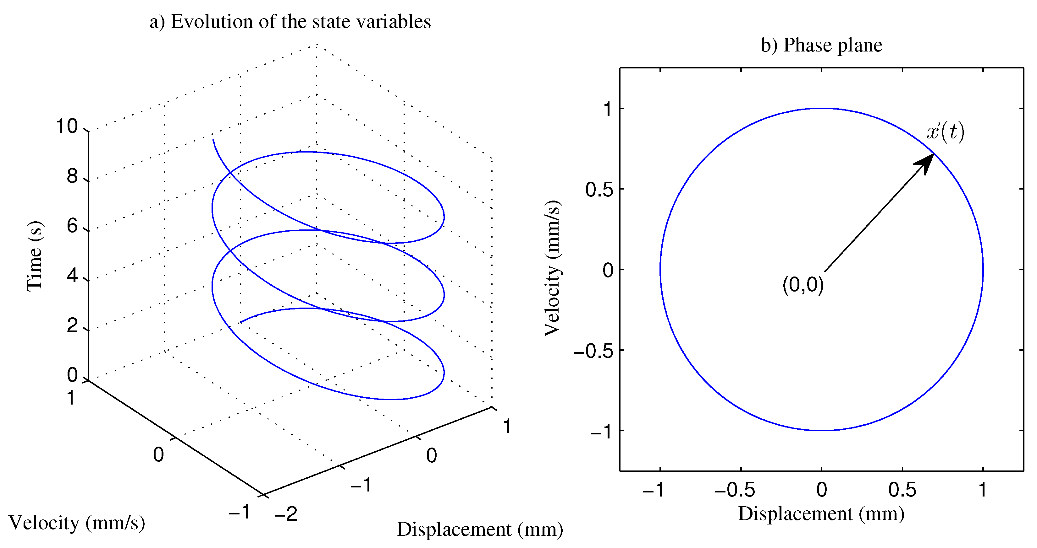
2.1. Phase Plane
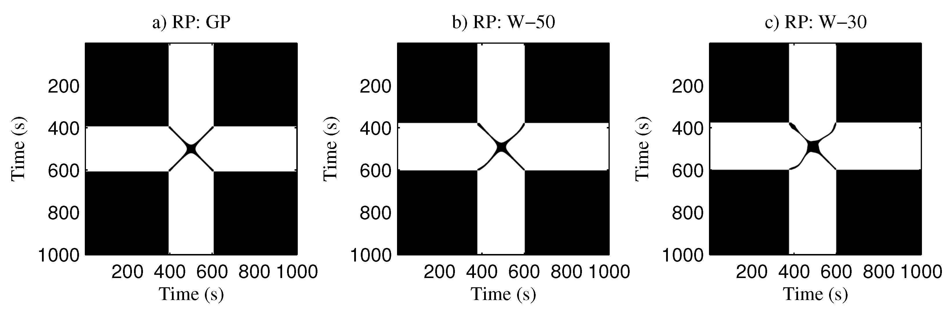
2.2. Recurrence Plot
3. Results
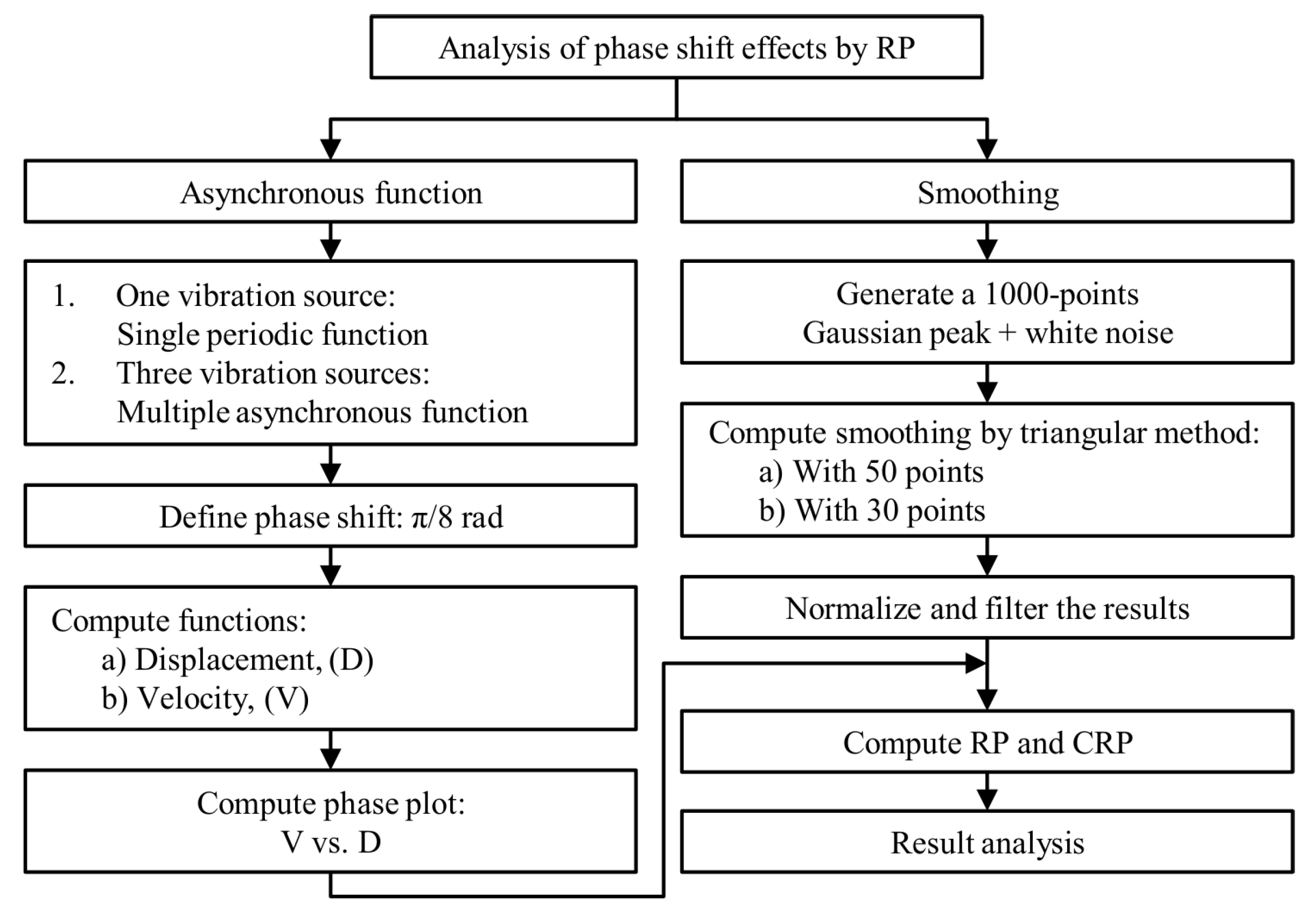
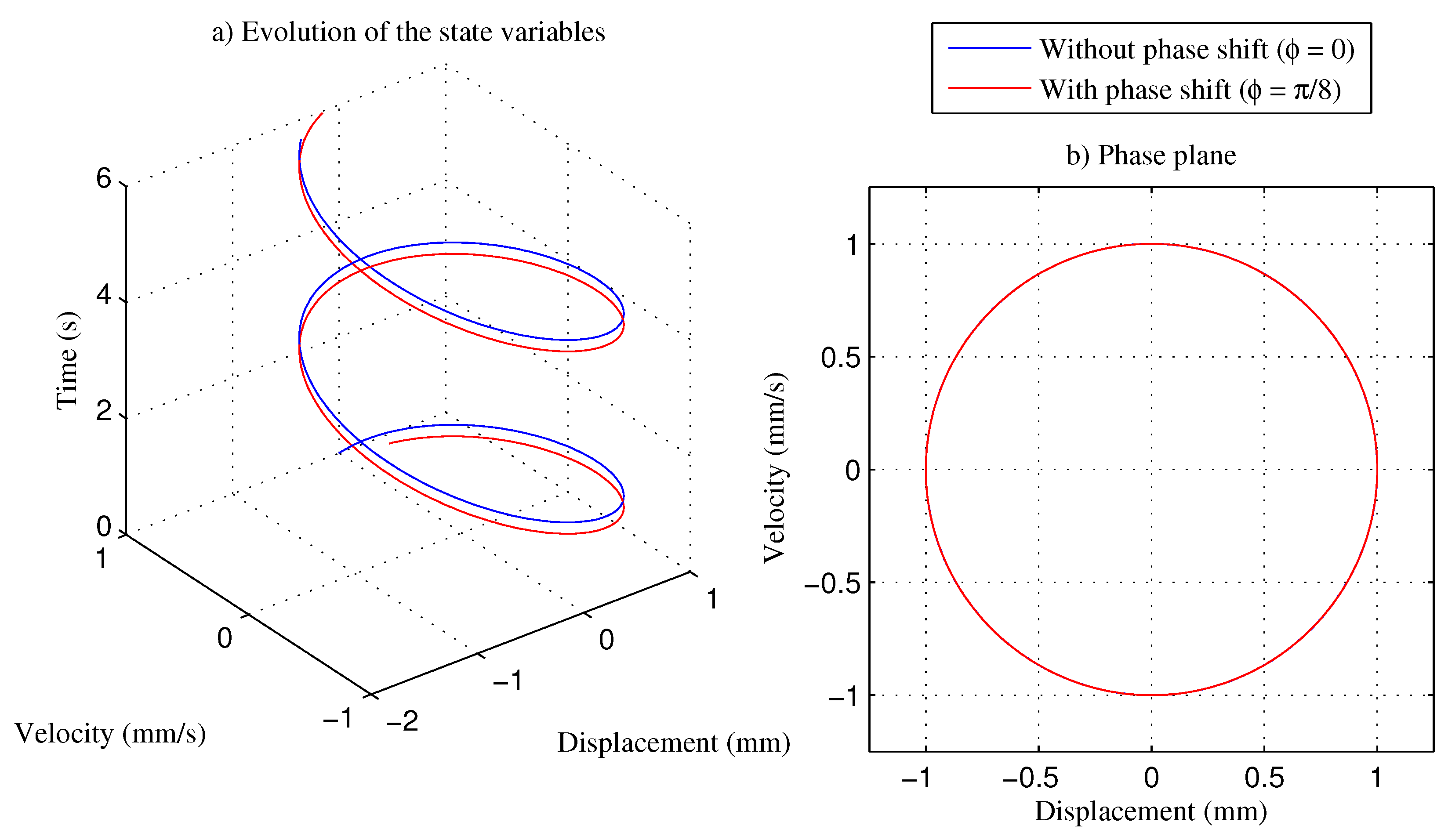
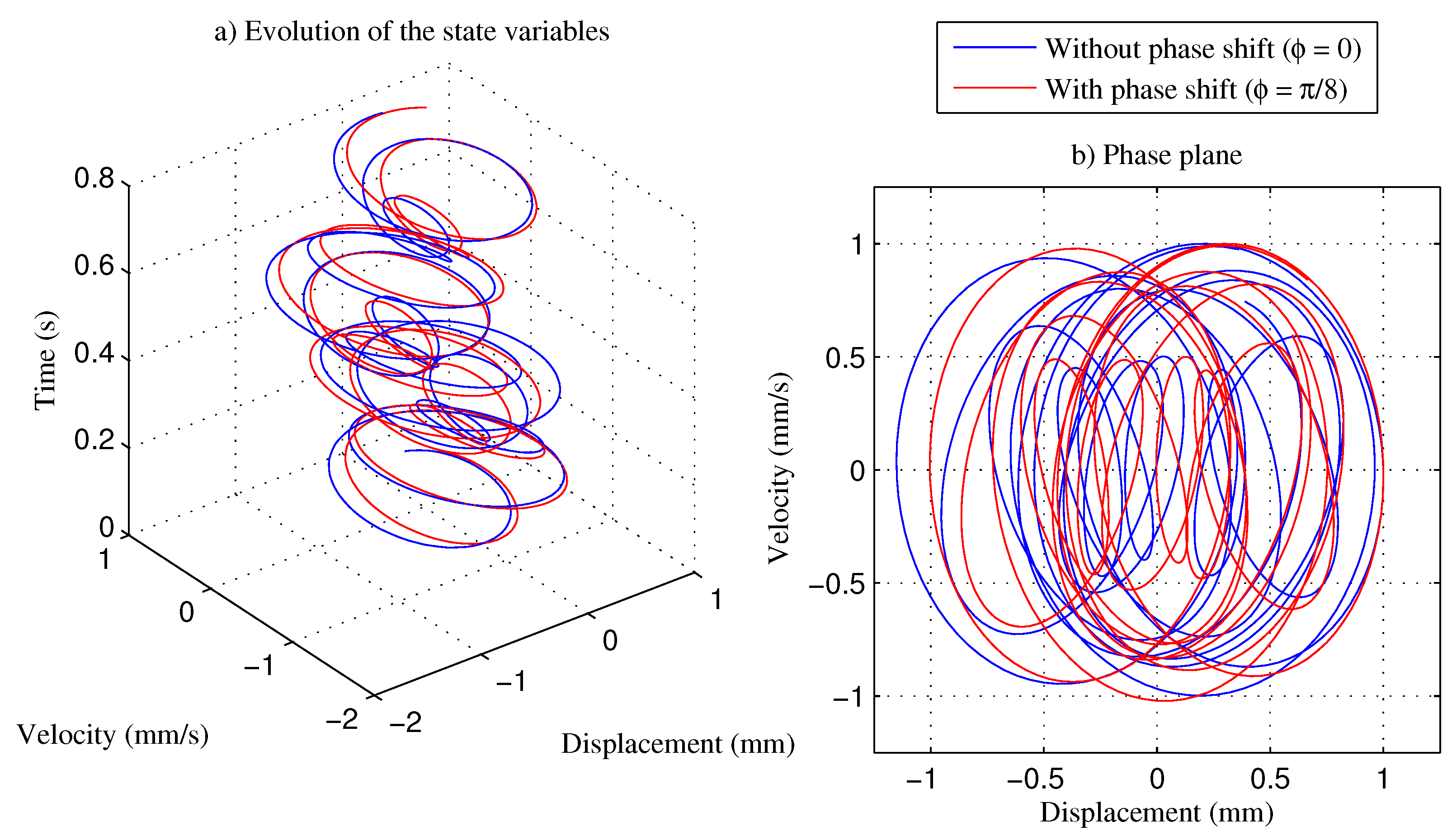
3.1. Phase Shift Effects on Multi-Source Functions
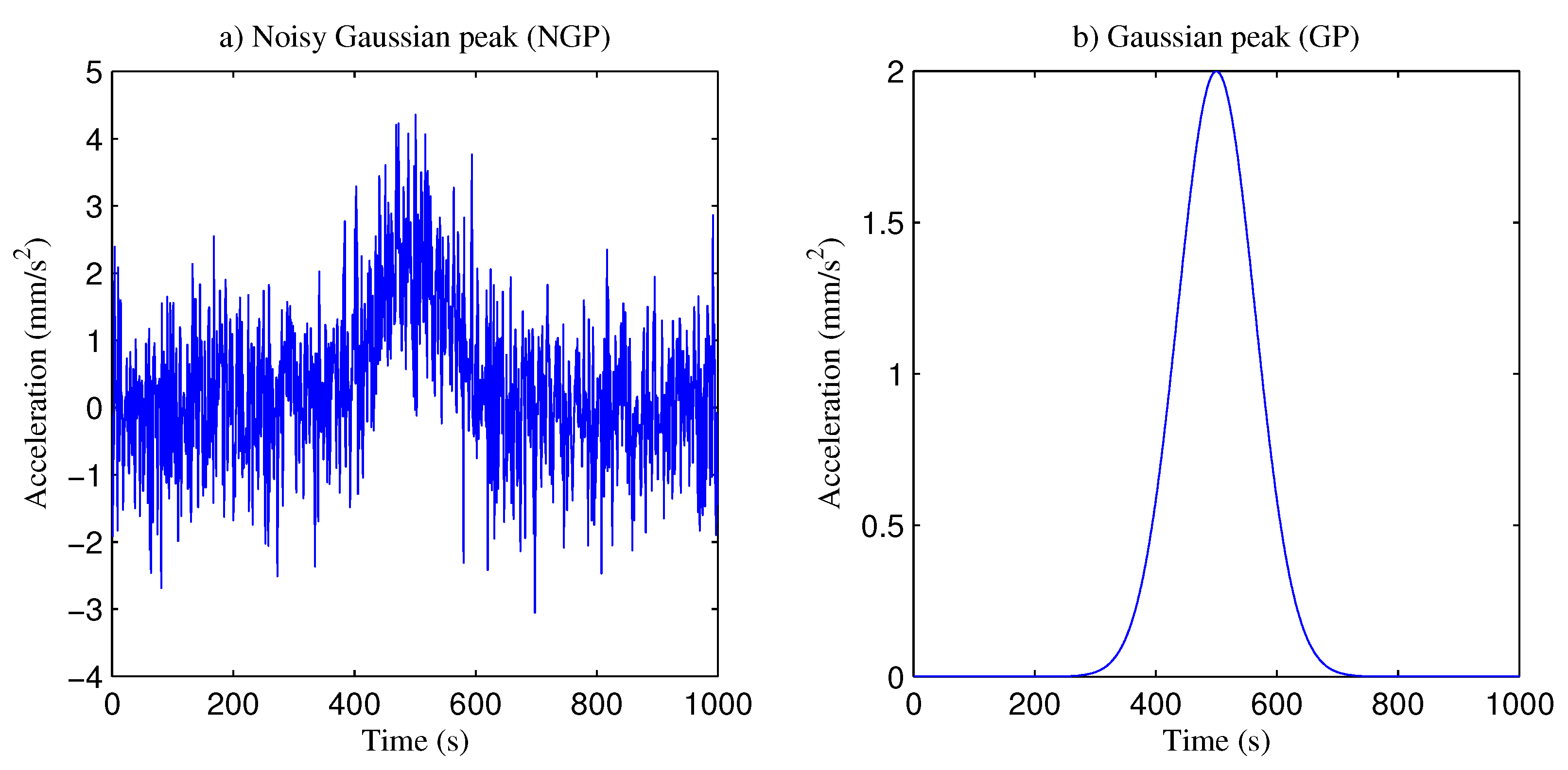
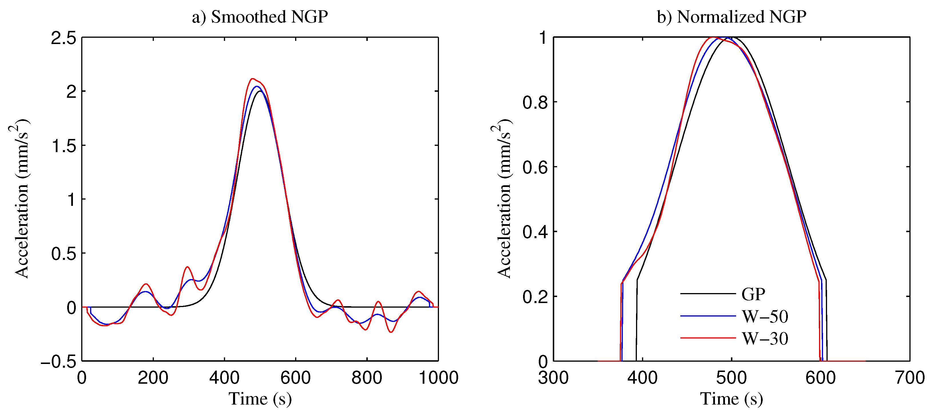
3.2. Smoothing Signal
4. Conclusions
Author Contributions
Funding
Conflicts of Interest
References
- Bokde, N.; Feijóo, A.; Villanueva, D.; Kulat, K. A Review on Hybrid Empirical Mode Decomposition Models for Wind Speed and Wind Power Prediction. Energies 2019, 12, 254. [Google Scholar] [CrossRef]
- Li, Y.; Wang, L. A novel noise reduction technique for underwater acoustic signals based on complete ensemble empirical mode decomposition with adaptive noise, minimum mean square variance criterion and least mean square adaptive filter. Def. Technol. 2020, 16, 543–554. [Google Scholar] [CrossRef]
- Poincaré, H. On the problem of the three bodies and the equations of dynamics. Acta Math. 1890, 13, 1–270. [Google Scholar]
- Eckmann, J.; Oliffson, S.; Ruelle, D. Recurrence Plots of Dynamical Systems. World Sci. Ser. Nonlinear Sci. Ser. A 1995, 16, 441–446. [Google Scholar]
- Pham, T. Fuzzy recurrence plots. In EPL Europhysics Letters; IOP Publishing: Bristol, UK, 2016; Volume 116. [Google Scholar]
- Marwan, N.; Romano, M.; Thiel, M.; Kurths, J. Recurrence plots for the analysis of complex systems. Phys. Rep. 2007, 438, 237–329. [Google Scholar] [CrossRef]
- Marwan, N.; Schinke, S.; Kurths, J. Recurrence plots 25 years later—Gaining confidence in dynamical transitions. EPL (Europhys. Lett.) 2013, 101, 20007. [Google Scholar] [CrossRef]
- Zhang, E.; Shan, D.; Li, Q. Nonlinear and Non-Stationary Detection for Measured Dynamic Signal from Bridge Structure Based on Adaptive Decomposition and Multiscale Recurrence Analysis. Appl. Sci. 2019, 9, 1302. [Google Scholar] [CrossRef]
- Acharya, U.; Faust, O.; Ciaccio, E.; Wei, K.; Lih, O.; Tan, R.; Garan, H. Application of nonlinear methods to discriminate fractionated electrograms in paroxysmal versus persistent atrial fibrillation. Comput. Methods Programs Biomed. 2019, 175, 163–178. [Google Scholar] [CrossRef]
- Yan, R.; Qian, Y.; Huang, Z.; Gao, R. Recurrence plot entropy for machine defect severity assessment. Smart Struct. Syst. 2013, 11, 299–314. [Google Scholar] [CrossRef]
- Qian, Y.; Yan, R.; Hu, S. Bearing Degradation Evaluation Using Recurrence Quantification Analysis and Kalman Filter. IEEE Trans. Instrum. Meas. 2014, 6, 2599–2610. [Google Scholar] [CrossRef]
- Chegini, S.; Manjili, M.; Bagheri, A. New fault diagnosis approaches for detecting the bearing slight degradation. Meccanica 2020, 55, 261–286. [Google Scholar] [CrossRef]
- Syta, A.; Litak, G. Vibration Analysis in Cutting Materials. In Recurrence Quantification Analysis, Understanding Complex Systems; Springer: Berlin/Heidelberg, Germany, 2015; pp. 279–290. [Google Scholar]
- Lajmert, P.; Rusinek, R.; Kruszyński, B. Chatter identification in milling of Inconel 625 based on recurrence plot technique and Hilbert vibration decomposition. In Proceedings of the International Conference on Engineering Vibration (ICoEV 2017), Sofia, Bulgaria, 4–7 September 2017; EDP Sciences: Les Ulis, France, 2018. [Google Scholar]
- Jauregui-Correa, J.; Camacho, S.; Basaldua-Sanchez, J. Bearing Analysis of the effect of different friction models on the dynamic response of a rotor rubbing the housing. Adv. Mech. Mach. Sci. Mech. Mach. Sci. 2019, 73, 4227–4236. [Google Scholar]
- Jauregui-Correa, J. Identification of Nonlinearities in Mechanical Systems Using Recurrence Plots. In Nonlinear Structural Dynamics and Damping, Mechanisms and Machine Science; Springer: Cham, Switzerland, 2019; Volume 69. [Google Scholar]
- Ferrero, R.; Galindo, F.; Montrucchio, B.; Rebaudengo, M. Exploiting accelerometers to estimate displacement. In Proceedings of the 5th Mediterranean Conference on Embedded Computing (MECO), Bar, Montenegro, 12–16 June 2016; pp. 206–210. [Google Scholar]
- Han, S. Measuring displacement signal with an accelerometer. J. Mech. Sci. Technol. 2010, 24, 1329–1335. [Google Scholar] [CrossRef]
- Yang, Y.; Zhao, Y.; Kang, D. Integration on acceleration signals by adjusting with envelopes. J. Meas. Eng. 2016, 4, 117–121. [Google Scholar]
- Liu, J.; Wang, P.; Tian, X. Vibration displacement measurement based on three axes accelerometer. In Proceedings of the Chinese Automation Congress, Jinan, China, 20–22 October 2017; pp. 2374–2378. [Google Scholar]
- Tezcan, J.; Marin-Artieda, C. Least-Square-Support-Vector-Machine-based approach to obtain displacement from measured acceleration. Adv. Eng. Softw. 2017, 115, 357–362. [Google Scholar] [CrossRef]
- Pan, C.; Zhang, R.; Luo, H.; Shen, H. Baseline correction of vibration acceleration signals with inconsistent initial velocity and displacement. Adv. Mech. Eng. 2018, 8, 1687814016675534. [Google Scholar] [CrossRef]
- Zhang, J.; He, Y. Removing baseline drift in vibration signal of autopilot based on morphology. Aeronaut. Astronaut. 2018, 44, 907–913. [Google Scholar]
- Kim, W.; Lee, H. An improved explicit time integration method for linear and nonlinear structural dynamics. Comput. Struct. 2018, 206, 42–53. [Google Scholar] [CrossRef]
- Wan, S.; Zhang, X.; Dou, L. Compound fault diagnosis of bearings using improved fast spectral kurtosis with VMD. J. Mech. Sci. Technol. 2018, 32, 5189–5199. [Google Scholar] [CrossRef]
- Zheng, W.; Dan, D.; Cheng, W.; Xia, Y. Real-time dynamic displacement monitoring with double integration of acceleration based on recursive least squares method. Measurement 2019, 141, 460–471. [Google Scholar] [CrossRef]
- Xu, J.; Xu, X.; Cui, X. A new recursive Simpson integral algorithm in vibration testings. Aust. J. Mech. Eng. 2019, 1–7. [Google Scholar] [CrossRef]
- Dela Cruz, A.; Cajayon, C.; Luna, J.; Tomboc, C. Recursive least square and least means square equalizers optimization algorithms in Rayleigh fading. Int. J. Adv. Trends Comput. Sci. Eng. 2019, 8, 689–695. [Google Scholar] [CrossRef]
- Ni, C.; Lin, T.; Xing, J.; Xue, J. A time-frequency analysis of non-stationary signals using variation mode decomposition and synchrosqueezing techniques. In Proceedings of the Prognostics and System Health Management Conference (PHM-Qingdao), Qingdao, China, 25–27 October 2019; pp. 1–6. [Google Scholar]
- Arrieta, M.; Kuar, R.; Zamora-Mendez, D. Identification of electromechanical oscillatory modes based on variational mode decomposition. Electr. Power Syst. Res. 2019, 167, 71–85. [Google Scholar] [CrossRef]
- Ribeiro, J.; de Castro, J.; Meggiolaro, M. Parameter adjustments for optimizing signal integration using the FFT-DDI method. J. Braz. Soc. Mech. Sci. Eng. 2020, 42, 104. [Google Scholar] [CrossRef]
- ZZhu, H.; Zhou, Y.; Hu, Y. Displacement reconstruction from measured accelerations and accuracy control of integration based on a low-frequency attenuation algorithm. Soil Dyn. Earthq. Eng. 2020, 133, 106122. [Google Scholar] [CrossRef]
- Chen, X.; Feng, Z. Induction motor stator current analysis for planetary gearbox fault diagnosis under time-varying speed conditions. Mech. Syst. Signal Process. 2020, 140, 106691. [Google Scholar] [CrossRef]
- Capobianco, R. A note on a practical relationship between filter coefficients and scaling and wavelet functions of Discrete Wavelet Transforms. Appl. Math. Lett. 2011, 24, 1257–1259. [Google Scholar]
- Guariglia, E.; Silvestrov, S. Fractional-Wavelet Analysis of Positive definite Distributions and Wavelets on D’(C). In Engineering Mathematics II; Silvestrov, S., Rančić, M., Eds.; Springer: Cham, Switzerland, 2016; Volume 179, pp. 337–353. [Google Scholar]
- Zheng, X.; Tang, Y.; Zhou, J. Framework of Adaptive Multiscale Wavelet Decomposition for Signals on Undirected Graphs. Graphs IEEE Trans. Signal Process. 2019, 7, 1696–1711. [Google Scholar] [CrossRef]
- Guariglia, E. Entropy and Fractal Antennas. Entropy 2016, 18, 84. [Google Scholar] [CrossRef]
- Guariglia, E. Primality, Fractality, and Image Analysis. Entropy 2019, 21, 304. [Google Scholar] [CrossRef]
- Marwan, N. CRP Toolbox. Potsdam Institute for Climate Reports. 2020. Available online: www.recurrence-plot.tk (accessed on 14 January 2021).
- Polyak, M. Phase-plane method: A practical approach. In Proceedings of the XII International forum Modern Information Society Formation—Problems, Perspectives, Innovation Approaches, Saint Petersburg, Russia, 6–11 June 2011; pp. 55–59. [Google Scholar]
- Polyak, M. Phase-plane method: A practical approach. J. Biomech. 2018, 73, 243–248. [Google Scholar]
- O’Haver, T. Pragmatic Introduction to Signal Processing 2019: Applications in Scientific Measurement; Independently Published, 2018; 459p, ISBN 10: 1792867123. [Google Scholar]


| Parameter | For | For | Variation (%) |
|---|---|---|---|
| 0.1 | 0.1 | 0 | |
| 1.0 | 1.0 | 0 | |
| 11.3 | 11.4 | 1 | |
| 499.0 | 499.0 | 0 | |
| L | 2.6 | 2.6 | 0 |
| 1.0 | 1.0 | 0 | |
| 9.8 | 9.8 | 0 | |
| 45.0 | 46.0 | 2 |
| Parameter | For | For | Variation (%) |
|---|---|---|---|
| 0.1 | 0.1 | 0 | |
| 0.9 | 0.9 | 0 | |
| 3.6 | 3.6 | 0 | |
| 196.0 | 229.0 | 17 | |
| L | 1.5 | 1.5 | 0 |
| 1.0 | 1.0 | 0 | |
| 3.8 | 3.9 | 3 | |
| 28.0 | 27.0 | −4 |
| Parameter | W–50 | W–30 | Variation (%) |
|---|---|---|---|
| 0.6 | 0.6 | 0 | |
| 1.0 | 1.0 | 0 | |
| 5.8 | 5.8 | 0 | |
| 1.0 | 1.0 | 0 | |
| L | 176.5 | 174.9 | −0.9 |
| 435.0 | 389.0 | −10.6 | |
| 232.1 | 132.6 | 0.2 | |
| 401.0 | 389.0 | −3.0 |
Publisher’s Note: MDPI stays neutral with regard to jurisdictional claims in published maps and institutional affiliations. |
© 2021 by the authors. Licensee MDPI, Basel, Switzerland. This article is an open access article distributed under the terms and conditions of the Creative Commons Attribution (CC BY) license (http://creativecommons.org/licenses/by/4.0/).
Share and Cite
Torres-Contreras, I.; Jáuregui-Correa, J.C.; López-Cajún, C.S.; Echeverría-Villagómez, S. Effects of Phase Shift Errors in Recurrence Plot for Rotating Machinery Fault Diagnosis. Appl. Sci. 2021, 11, 873. https://doi.org/10.3390/app11020873
Torres-Contreras I, Jáuregui-Correa JC, López-Cajún CS, Echeverría-Villagómez S. Effects of Phase Shift Errors in Recurrence Plot for Rotating Machinery Fault Diagnosis. Applied Sciences. 2021; 11(2):873. https://doi.org/10.3390/app11020873
Chicago/Turabian StyleTorres-Contreras, Ignacio, Juan Carlos Jáuregui-Correa, Carlos Santiago López-Cajún, and Salvador Echeverría-Villagómez. 2021. "Effects of Phase Shift Errors in Recurrence Plot for Rotating Machinery Fault Diagnosis" Applied Sciences 11, no. 2: 873. https://doi.org/10.3390/app11020873
APA StyleTorres-Contreras, I., Jáuregui-Correa, J. C., López-Cajún, C. S., & Echeverría-Villagómez, S. (2021). Effects of Phase Shift Errors in Recurrence Plot for Rotating Machinery Fault Diagnosis. Applied Sciences, 11(2), 873. https://doi.org/10.3390/app11020873