Article

An Improved Collaborative Filtering Recommendation Algorithm Based on Retroactive Inhibition Theory

Key Laboratory of Trustworthy Distributed Computing and Service, Ministry of Education, School of Computer Science (National Pilot Software Engineering School), Beijing University of Posts and Telecommunications, Beijing 100876, China
*
Author to whom correspondence should be addressed.
Appl. Sci. 2021, 11(2), 843; https://doi.org/10.3390/app11020843
Submission received: 29 November 2020 / Revised: 2 January 2021 / Accepted: 13 January 2021 / Published: 18 January 2021

Abstract

:
Collaborative filtering (CF) is the most classical and widely used recommendation algorithm, which is mainly used to predict user preferences by mining the user’s historical data. CF algorithms can be divided into two main categories: user-based CF and item-based CF, which recommend items based on rating information from similar user profiles (user-based) or recommend items based on the similarity between items (item-based). However, since user’s preferences are not static, it is vital to take into account the changing preferences of users when making recommendations to achieve more accurate recommendations. In recent years, there have been studies using memory as a factor to measure changes in preference and exploring the retention of preference based on the relationship between the forgetting mechanism and time. Nevertheless, according to the theory of memory inhibition, the main factors that cause forgetting are retroactive inhibition and proactive inhibition, not mere evolutions over time. Therefore, our work proposed a method that combines the theory of retroactive inhibition and the traditional item-based CF algorithm (namely, RICF) to accurately explore the evolution of user preferences. Meanwhile, embedding training is introduced to represent the features better and alleviate the problem of data sparsity, and then the item embeddings are clustered to represent the preference points to measure the preference inhibition between different items. Moreover, we conducted experiments on real-world datasets to demonstrate the practicability of the proposed RICF. The experiments show that the RICF algorithm performs better and is more interpretable than the traditional item-based collaborative filtering algorithm, as well as the state-of-art sequential models such as LSTM and GRU.

1. Introduction

Since the inception of the Internet, users and hardware devices have generated an enormous amount of data. The problem of “information overload” has inevitably emerged, and recommendation algorithms have to solve the problem of how to efficiently extract valuable information from these massive amounts of unorganized data. Therefore, there is no doubt that recommendation systems, as the engines of Internet development, provide great convenience and benefits to users and Internet companies in the “information overload” era. They have also seen success in e-commerce and social networking as well as other fields.
The most traditional and widely used recommendation algorithm is the collaborative filtering algorithm (abbreviated as CF), which is further divided into item-based collaborative filtering (abbreviated as itemCF) and user-based collaborative filtering (abbreviated as userCF) algorithm based on item similarity and user similarity, so as to calculate the ratings of unknown items as well as predict user preferences. For example, for a target item whose rating needs to be estimated, the userCF chooses to calculate the similarity between users, and then the unknown rating is predicted by averaging the (weighted) known ratings of the target item by similar users. On the other hand, the itemCF calculates the similarity between items first and then predicts the unknown rating by averaging the (weighted) known ratings of similar items by other users [1,2]. As shown in Figure 1, according to user’s movie-watching history, user a and user b share preferences, so the userCF recommends movie 3 and movie 6, which user a likes, to user b . Meanwhile, the itemCF recommends movie 2, which is similar to movie 6 that user b liked before, to user b .
CF algorithms are all designed to recommend items to users based on the preferences of similar users or the user’s history, and the process is done by calculating the similarity between users or items. However, traditional CF algorithms suffer from the problem of data sparsity and inadequate exploration of mechanisms of how user preferences decay. In fact, several prior studies [3,4,5] pointed out that preference decay and memory decay are very similar. Thus, this paper proposes an improved CF algorithm based on retroactive inhibition of preferences (abbreviated as RICF) to capture the evolution of user’s preferences. There are a number of papers in the field of recommendation systems that measure the memory forgetting process based directly on the decay of time [6,7,8,9]. However, according to the [10,11,12] researches in psychology, memory attenuation mainly stems from memory inhibition. Therefore, RICF adopts the theory of retroactive inhibition, which measures the retention of the user’s preference on item a by calculating the strength of inhibition that item a suffered within the corresponding time period, and consequently affects the weight of the contribution that item a makes to the target item’s rating prediction.
For example, given samples as in Table 1, to predict user a ’s rating of movie 4 on 11/12/2018, traditional itemCF calculates the contribution of each similar movie directly (namely, rating × similarity), so user a ’s rating of movie 1 has contributed 2.5 × 0.9 = 2.25 rating to the prediction of user a ’s rating of movie 4. However, we need to adjust the user’s previous ratings to fit real scenarios because of the evolution of user’s preference. Specifically, on 11/12/2018, for the preference that user a had to movie 1, it suffered retroactive inhibition from 05/04/2018 to 11/12/2018, namely the inhibition from movie 3 rated by user a , which exists in a different preference cluster and has a higher rating. Movie 3 subsequently affects movie 1’s contribution to the prediction of movie 4’s rating (2.5 × 0.9 × D e c a y ( R I ) ). In this way, RICF measures the evolution of user’s preferences more interpretatively and accurately from the perspective of preference inhibition.
The contributions of this paper are described as follows,
  • This paper introduces the theory of retroactive inhibition into recommendation systems to more interpretably measure the decay of a user’s preference over time. Specifically, we modified the application of the forgetting mechanism of brain memory to the recommendation system by using retroactive inhibition instead of using forgetting over time directly, in order to calculate the change of user’s preference more accurately.
  • The proposed RICF algorithm not only takes into account the evolution of user preferences but also uses more powerful item embeddings by fusing user, item and rating information to alleviate the problem of data sparsity and improve the accuracy of rating prediction. In addition, the embeddings trained by the model (using rating-prediction as an optimization goal) can help to reduce the number of similar neighbors in the collaborative process.
  • Differing from previous related studies, this paper proposes to use a clustering of embeddings to obtain a preference points model. Meanwhile, RICF combines the Canopy and K-Means algorithms to overcome the problem that the clustering efficiency decreases with the increasing size of the dataset, as well as the feature dimension.
  • To show the practicability of the proposed algorithm, this paper applies real datasets with real timestamps, which are the live movie rating dataset collected from Twitter [13] and the digital music dataset collected from Amazon [14]. The experiment results show that RICF performs better and is more interpretable than the traditional itemCF as well as the state-of-the-art sequential algorithms that focus on the research of preference decay.
The remainder of this paper is organized as follows. Section 2 summarizes the related work. Section 3 provides some preliminaries and describes the proposed RICF algorithm. Section 4 presents results from experiments conducted on two evaluation datasets. Section 5 concludes the paper.

2. Related Work

2.1. Collaborative Filtering Recommendation

Recommendation System (RS) plays an important role in today’s Internet, which aims to filter relevant as well as important information for users from previous feedbacks. The demand for such systems is gradually increasing along with the overload of data on the Internet. The root of RS can be traced back to the extensive researches in cognitive science [15], information retrieval [16], management science [17], and also in consumer choice modeling in marketing [18]. Later on, RS developed into an independent research field in the mid-1990s to tackle problems in the structure of explicit rating [19]. Naturally, one of the most common processes is to turn recommendations into operations to predict an unknown item’s rating for users based on their previous behaviors, namely, the rating-prediction problem. Then, we can recommend the highest rated items to the user based on the predictions. In addition, there are top-N based recommendations, but this paper mainly focuses on the problem of rating prediction. Moreover, the approaches of RS can be divided into three categories [19]: (1) content-based recommendation, (2) collaborative recommendation, and (3) hybrid approaches.
CF algorithms belong to the collaborative recommendation, which makes recommendations similar to user’s previous preference or from similar users. According to [20], algorithms for collaborative recommendations can be grouped into two general classes: memory-based(or heuristic-based) and model-based. Memory-based algorithms [20,21,22] are essentially heuristics that make recommendations based on the entire dataset of user previous behaviors, which can be further divided into userCF and itemCF. Furthermore, [23,24] present empirical evidence that itemCF can provide better computational performance as well as better quality of recommendation than traditional userCF. On the other hand, model-based algorithms [25,26,27,28,29,30] focus on model learning and then apply the trained model to the recommendation. Meanwhile, there are two popular error functions for CF algorithms to evaluate the performance, especially for the task of rating prediction: mean absolute error (MAE) and root mean squared error (RMSE). Since the absolute value function is not differentiable at all points, RMSE is more desirable as an objective function [31].
However, traditional CF algorithms suffer from different problems: sparsity, high dimensionality of data [32], and disability of capturing the evolution of user preferences over time. From now on, amounts of researches in the recommendation community have emerged to tackle these difficulties. For example, to tackle the first problem, [33] directly reduce the number of users/items, [34,35] extract information from clustered groups, and more advanced, [36,37] propose to learn a latent space vector for each user/item by deep learning algorithms. On the second problem, to the best of our knowledge, there are two main different solutions that take user’s dynamic preferences into consideration. One way is to directly apply time as a factor [7,8,38,39], e.g., Ebbinghaus’s forgetting curve. Another approach is driven by the development of sequential recommendation, which treats user-item interactions as a series of sequential events and takes the sequential dependencies into account to capture user’s current or recent preference for more accurate recommendations [40], such as state-of-art techniques, Long Short Term Memory (LSTM) [41,42] and Gated Recurrent Unit (GRU) [43].
In summary, the fact of reducing the influence of data sparsity as well as emphasizing the requirement of capturing dynamic user’s preferences has gained more attention in the recommendation field. The classic CF algorithm still faces these challenges, and these factors should be taken into account to make recommendations not only interpretable but more accurate. Thus, that is the direction we follow in this paper.

2.2. Retroactive Inhibition Theory

Inhibition is one of the core concepts in Cognitive Psychology [11]. The idea that inhibition actively impairs the representation of the human mind has inspired a great deal of research in various fields. Specifically, among the several theories of the forgetting mechanism, the overall evidence suggests that the inhibition within similar objects are by far the most critical factor in the forgetting process rather than the direct time factor [11,44]. In addition, inhibition theory, also known as interference theory, proposed that information competition can refer to either proactive inhibition (PI) (interfered by previous similar objects) or retroactive inhibition (RI) (interfered by subsequent similar objects) [45]. For example, after you learn a vocabulary list containing the word “dairy” and the word “diary” (the “dairy” was learned first and the “diary” was learned later), your recall of the two similar words will be affected by mutual inhibition. Proactive inhibition is the inhibition of newer memories with the retrieval of older memories, that is, your memory of “dairy” will produce proactive inhibition when you recall “diary”. Retroactive inhibition is the inhibition of older memories with the retrieval of newer memories, that is, your memory of “diary” will produce retroactive inhibition when you recall “dairy”. Compared with proactive inhibition, retroactive inhibition may have larger effects [46].
According to [11], algorithms should take the cognitive principles into consideration to be more in tune with the process of forgetting. However, for Computer Science, to the best of our knowledge, while the cognitive concept of activation propagation and the concept of forgetting have been adopted into different types of computer science approaches more recently, the explicit adoption of the concept of inhibition has not been investigated yet [11].

3. Proposed Model: RICF

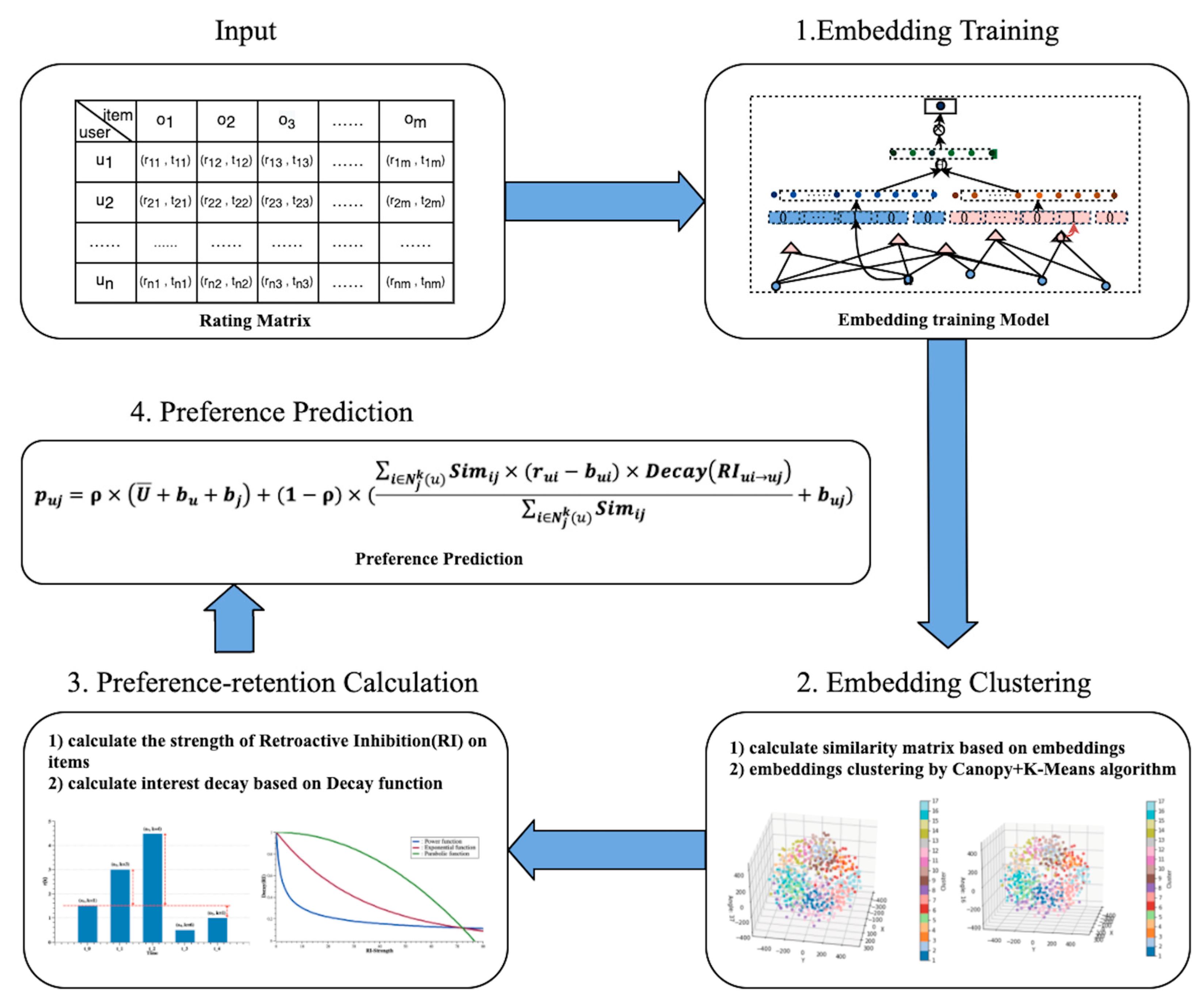
Similar to the example of learning words in Section 2.2, a user’s recall of the older preferences can be affected by the competing information in the memory of newer preferences, which leads to a memory bias towards the older preferences. Thus, in order to explore the bias of user’s preferences memory and improve the accuracy of rating prediction, this paper mainly focuses on the phenomenon of memory decay caused by competition-induced retroactive inhibition. Specifically, this paper introduces the retroactive inhibition factor (RI) and proposes the RICF algorithm to improve the traditional CF algorithm. The whole algorithm is divided into the following steps: (1) training embedding vectors; (2) embedding clustering; (3) preference-retention calculation; (4) preference prediction. The whole process is shown in the Figure 2.
To tackle the data sparsity problem, this paper introduces a deep learning technique, called embedding training, to convert high-dimensional sparse vectors of items into low-dimensional dense vectors. The distance between these trained embeddings reflects the similarity between them. Then, we clustered embeddings, and the clustered results represent the user’s preferences. After that, the evolution of the user’s preferences is shown by calculating the inhibition intensity and preference retention for each user’s historical preference. Finally, we calculated the user’s future preferences based on the evolution of the user’s preferences and the similarity between item embeddings.

3.1. Preliminary

Suppose that there are a user set U   =   { u 1 , u 2 u n } and an item set O   =   { o 1 , o 2 o m } , we define the rating pair ( r i j , t i j ) , where r i j represents the rating for user u i to item o j and t i j is the time when user u i rates item o j . The vector u i represents the rating pair set of user u i . If user u i does not rate item o j , then the corresponding rating pair is empty. Finally, the rating matrix M is defined as follows,
M   =   [ u 1 u 2 u i u n ]   =   [ ( r 11 , t 11 ) ( r 1 m , t 1 m ) ( r n 1 , t n 1 ) ( r n m , t n m ) ] ,
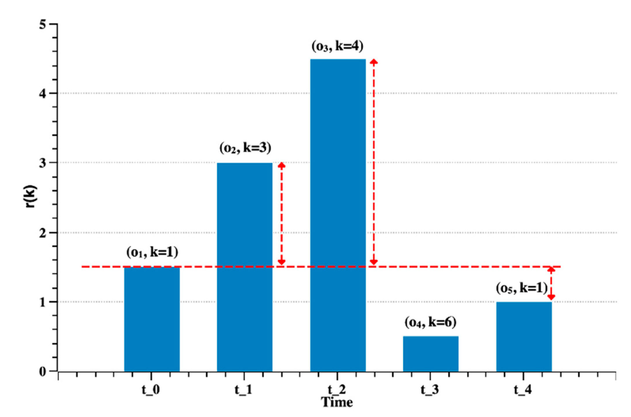
Definition 1 (Retroactive Inhibition Strength) is given an item set O   =   { o 1 , o 2 o m } and a user set U   =   { u 1 , u 2 u n } , then we can assign each item o j a label k to record the cluster (we call it the preference point) k it belongs to after concluding the clustering of items in the item set, considering the result of cluster shows the preference distribution of users. After that, the retroactive inhibition strength for item o n (belongs to the preference point k ) rated by user u i from time t i n to time t i m can be defined as follows,
R I i n i m   =   k K i n i m D i s t ( k , k ) ,
R I i n i m represents the total impact of retroactive inhibition on u i ’s preference on the preference point k that o n belongs to, where K i n i m in the Equation (2) is a collection of preference points to which u i ’s rated items belong from time t i n to time t i m . Moreover, retroactive inhibition is caused by the influence of other stronger preferences or the same preference from time t i n to time t i m , we defined the D i s t function to calculate preference distance between k and k for user u i , as shown in Equation (3).
D i s t ( k , k )   =   { 0 , r ( k )     r ( k )   a n d   k     k r ( k )     r ( k ) , r ( k )   >   r ( k )   a n d   k     k ( r ( k )     r ( k ) ) , k   =   k
where function r aims to measure the cumulative strength of a user’s preference for a particular preference point within the specified time period. Specifically, r ( k ) is the function to get the average rating among the rating records which rated from time t i n to time t i m with the preference point k , and r ( k ) is the function to get the average rating among the rating records that rated earlier than t i n with the preference point k .
For example, assuming that user u i rated items { o 1 , o 2 , o 3 , o 4 , o 5 } sequentially, and we know that items fell into preference points { k   =   1 , k   =   3 , k   =   4 , k   =   6 , k   =   1 } , respectively, as shown in Figure 3. Then, according to Equation (3), we can calculate the impact of retroactive inhibition on user’s preference on o 1 (which belongs to k   =   1 ), namely R I i 1 i 5   =   ( 3.0 1.5 ) + ( 4.5 1.5 ) + 0 + ( ( 1.0 1.5 ) )   = 4 .

3.2. Embedding Training

According to Section 2.1, traditional collaborative filtering techniques also have the problem of data sparsity and insufficient expression of features of data. That is, a small proportion of items rated by a few users, and other information such as interactions between users and items, sequential information, fail to be represented in traditional CF algorithms. Therefore, inspired by the “item2vec” method [36], this paper proposes to pre-train a model based on the feedforward deep neural network with ratings as an optimization target to get the dense numeric representations for users/items, which aims to obtain more accurate representations of users/items in the rating space.
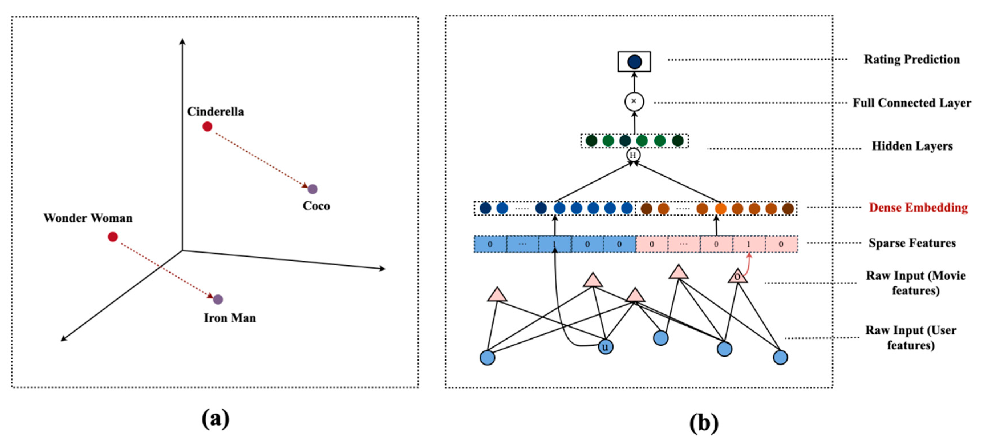
More generally, the conversion that makes the original features of an item be transformed into a dense item embedding vector is called “item2vec”. Thus, we train the aforementioned model which inputs users and items information into it, and makes ratings as optimization targets. Consequently, the original features of users/items are transformed into a dense user/item embedding vector, namely V e c ( u i )   =   { w 1 , w 2 w n } and V e c ( o i )   =   { w 1 , w 2 w m } , where n and m are the dimensions of the embedding vector. The whole architecture is shown in Figure 4b. Specifically, for example, the proposed model maps each movie in the dataset to a dense (embedded) vector in a unified Euclidean space where the distance inside represents some kind of correlation between movies, as in Figure 4a, exploring some implicit information between embeddings in vector space by the tool Gensim [47]. It can be seen that the distance vectors from the movie Wonder Woman (a female-themed sci-fi movie) to movie Iron Man (a male-themed sci-fi movie) and from movie Cinderella (a female-themed fantasy movie) to movie Coco (a male-themed fantasy movie) are almost identical, suggesting that the embedding operation in this example can contain the rating relationship and some semantic information among rating history.
We have applied the “item2vec” method to CF to overcome the sparse data problem and take full advantage of the powerful expression of embeddings at the same time to accurately calculate the similarity between items, so that we can achieve more accurate preference predictions that will be discussed in the next sections.

3.3. Embedding Clustering

In addition to solving the data sparsity problem and measuring the similarity between items more precisely, we use clustering of embeddings to better explore the user’s preference partitions, and thus obtain the set of user’s preference points, see Definition 1. Furthermore, in contrast to the K-Means algorithm, the Canopy+K-Means algorithm is used to solve the problem where the effect of clustering for multidimensional data is limited by the K-value and the initial cluster centers, as well as the problem of slow computation of using the K-Means algorithm.
(1)
Canopy coarse clustering
Canopy is an extremely simple and fast pre-processing algorithm. It was first proposed by Andrew McCallum, Kamal Nigam and Lyle Ungar in 2000 [48]. It is often used for coarse clustering before K-Means algorithm to find appropriate K-value and initial cluster centers [49] for K-Means algorithm. Specifically, it applies the inexpensive distance method to rough clustering and rigorous distance method to standard clustering. In this way, the Canopy algorithm can make large and high-dimensional data clusters efficiently and practically [50]. Inspired by the Canopy algorithm, this paper proposes to pre-process the embeddings using the Canopy algorithm to obtain the appropriate cluster K-value and the initial cluster centers which will be treated as input to the K-Means algorithm in the next step, so as to get better cluster results in less time.
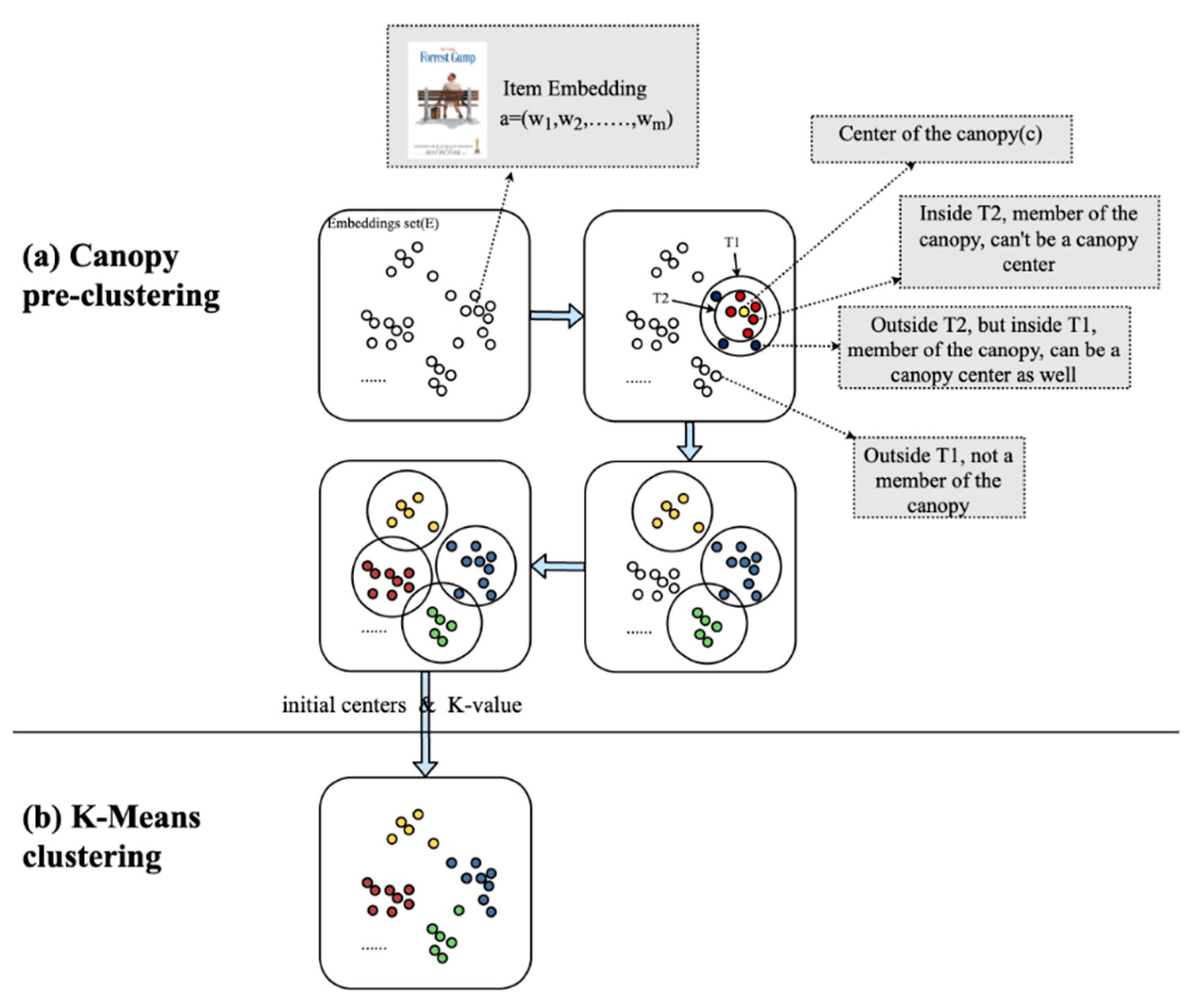
As shown in Figure 5, given that the set of item embeddings E (e.g., movie embeddings) and the heuristic threshold T 1 , T 2 for the Canopy algorithm. First, sample a is selected randomly from E to initialize Canopy c , then the distance between a and the remaining samples in E is calculated. Second, assign those samples of the distance within T 1 to Canopy c and remove those samples of the distance within T 2 from E . Repeat this process until the set E is empty. Last, return the number of canopies and centroids as the K-value as well as initial centroids of the K-Means algorithm.
Algorithm 1. Pseudocode for Canopy clustering algorithm for embeddings.
1:Input: the set of item embeddings E = { e 1 , e 2 , , e m }.
2:Output: the K-value and initial centroids S = { s 1 , s 2 , , s k } of cluster.
3:Initialize T 1 , T 2
4:while E do
5: Select sample a from E randomly
6: Initialize Canopy c a
7: Remove a from E
8:for remaining sample e E do
9:  compute d
10:  if d < T 1 then
11:   Canopy   c     e
12:else if d < T 2   then
13:   remove e from E
14:  end if
15:end for
16:end while
17:return K-value, initial centroids
(2)
K-Means clustering
After coarse clustering by the Canopy algorithm, the number of clusters K and cluster centers { s 1 , s 2 s k } are obtained, where each cluster center s i is a multidimensional vector with the same latitude as the item embedding. Then, we apply the traditional K-Means algorithm [51,52] by the incorporation of known K-value and initial centroids to cluster embeddings. Eventually, we get the result of the embeddings cluster, namely the set of user preference points.

3.4. Preference Retention Calculation

After Canopy+K-Means clustering, RICF uses the clustering results and the theory of retroactive inhibition to explore the evolution of user’s preferences. In addition, this is assuming that user u i rated items { o 1 , o 2 , o 3 , o 4 , o 5 } sequentially, as shown in Figure 3, and these items were partitioned in clusters { k = 1 , k = 2 , k = 4 , k = 6 , k = 1 } by Canopy+K-Means algorithm, respectively. Then, according to the definition of retroactive inhibition strength, we can calculate the suffered RI strength of each item. Consequently, R I i 1 i 5 = 4 , R I i 2 i 5 = 1.5 , R I i 3 i 5 = 0 , R I i 4 i 5 = 0.5 , R I i 5 i 5 = 0 .
Next, we need to define a RI-based decay function to simulate the process of user’s preferences decay due to memory inhibition. We name the described function as D e c a y ( R I ) to record the proportion of user’s preference retention. In addition, inspired by the Ebbinghaus Curve [11], we address several methods to find out the most appropriate simulation curve, including Power function, Exponential function and Parabolic function as a control for extreme conditions. As an instance shown in Figure 6.
So far, we can calculate the proportion of user’s preference retention on specific items by the defined decay function and RI strength. Consequently, user’s real preference can be measured to improve the accuracy as well as interpretation of the recommendation.

3.5. Preference Prediction

RICF improved the traditional itemCF algorithm based on the idea of retroactive inhibition to take user preference evolution into consideration, and it introduced baseline rating as well as adjusted methods to calculate the similarity between items directly on the item embeddings obtained from the previous training. The experiment results are shown in the next section.

Definition 2 Embedding Similarity

Based on the items for which the embeddings have been trained, this paper uses the Cosine method to calculate the similarity between the two embeddings V e c ( O x ) =   { x 1 , x 2 , x n } and V e c ( O y ) =   { y 1 , y 2 y n } . The original Cosine is used to calculate the angle θ between two vectors V e c ( O x ) and V e c ( O y ) , ranging from −1 to 1, as defined in Equation (4). The proposed RICF uses the normalized Cosine method to measure the similarity between two embedding vectors, as shown in Equation (5).
cos ( θ ) x y   =   V e c ( O x ) × V e c ( O y ) | V e c ( O x ) × V e c ( O y ) |   =   i   =   1 n x i y i i   =   1 n x i 2 × i   =   1 n y i 2 ,
S i m x y   =   1 + cos ( θ ) x y 2 ,
Consequently, this paper derives the RICF algorithm as follows, to predict user u i ’s preference for item o j .
p u j   =   ρ × ( U ¯ + b u + b j ) + ( 1 ρ ) × ( i N j k ( u ) S i m i j × ( r u i b u i ) × D e c a y ( R I u i u j ) i N j k ( u ) S i m i j + b u j )
where ρ is the heuristic parameter which we chose by stochastic selection strategy. Part 1 of this equation is the baseline rating, where U ¯ is the mean rating for all users. b u and b j are the rating bias of user u i and item o j , as defined in Equations (7) and (8), respectively. Moreover, in Equations (7) and (8), N ( u ) ( N ( j ) ) represents all rating records associated with user u (item o j ), r ¯ i ( r u ¯ ) represents the mean rating of item o i (user u ). Part 2 of Equation (6) is an improved itemCF algorithm that introduces embedding similarity S i m i j to calculate the similarity between item o i and item o j , as shown in Definition 2, and introduces preference decay factor D e c a y ( R I u i u j ) to calculate the decay degree of user u ’s preference on older items o i when user u is going to rate newer item o j , as seen in Section 3.4. Meanwhile, b u i   ( b u j ) is the simplified base rating prediction for item o i ( o j ), which equals r u ¯ + b i ( r u ¯ + b j ). What is more, the KNN part in Equation (6) chooses N j k ( u ) , which selects k items most similar to item o j from the rating history of user u .
b u   =   i N ( u ) r u i r i ¯ | N ( u ) |
b j   =   j N ( j ) r u j r u ¯ | N ( j ) |

4. Results and Discussion

This section shows the comparison between traditional methods and our proposed RICF algorithm. Several state-of-the-art algorithms are also implemented as baselines to compare with the proposed RICF algorithm.

4.1. Dataset and Experimental Setup

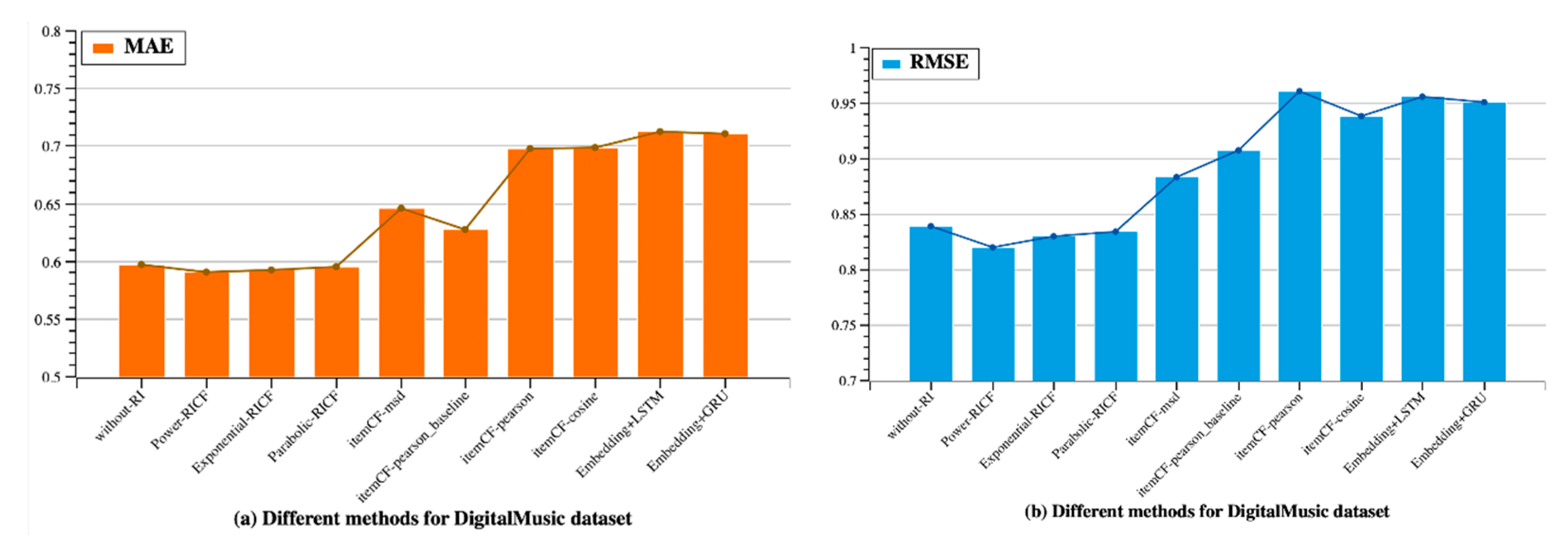
Specifically, to evaluate the performance of the proposed RICF algorithm, we designed a total of seven algorithms to be used as comparisons for the experiment: (1) traditional itemCF, (2) RICF excluding RI effects, namely D e c a y ( R I u i u j )   = 1 in Equation 6 (without-RI), (3) RICF with Power decay function (Power-RICF), (4) RICF with Exponential decay function (Exponential-RICF), (5) RICF with Parabolic decay function (Parabolic-RICF), (6) sequential model LSTM (Embedding+LSTM), and (7) sequential model GRU (Embedding+GRU). All algorithms are coded in python and tested on the Kaggle cloud-based workbench.
Furthermore, in order to ensure that each rating record is rated on user’s real rating habits and scenarios (not rated by volunteers at once such as in the Movielens dataset [53]) and thus to ensure the authenticity of user’s preference evolution, we have specially selected three well-known datasets based on real timestamps, MovieTweetings-100k, MovieTweetings-latest [13], and DigitalMusic [14] to conduct the experiment. MovieTweetings is an up-to-date dataset that collects all tweets from Twitter having the format “*I rated #IMDB*”. Originally, the MovieTweetings-100k contained 16,554 unique users and 10,506 unique movies that were rated from 28/02/2013 to 01/09/2013. Likewise, the MovieTweetings-latest contains 68,332 unique users and 35,931 unique items that were rated from 28/02/2013 to 10/07/2020. All of the movie ratings are scaled from 1 to 10, which will be re-scaled to 1 to 5 in this paper. The DigitalMusic dataset contains reviews and metadata from Amazon. It contains 478,235 unique users and 266,414 unique digital music that were rated from 20/01/1998 to 23/07/2014. All of the music ratings are scaled from 1 to 5. The description of these three datasets is as shown in Table 2.

4.2. Evaluation Metrics

Based on the common metrics of rating prediction in the recommendation system, this paper uses the mean absolute error (MAE) and the root mean squared error (RMSE), as metrics to evaluate how well we predict. They are defined as follows.
Assuming there are prediction values y ^   =   { y ^ 1 , y ^ 2 , , y ^ n } and target values y   =   { y 1 , y 2 , , y n } . Therefore,
R M S E   =   1 n i   =   1 n ( y ^ i y i ) 2 ,
M A E   =   1 n i   =   1 n | y ^ i y i | ,

4.3. Results

4.3.1. Recommendation Quality

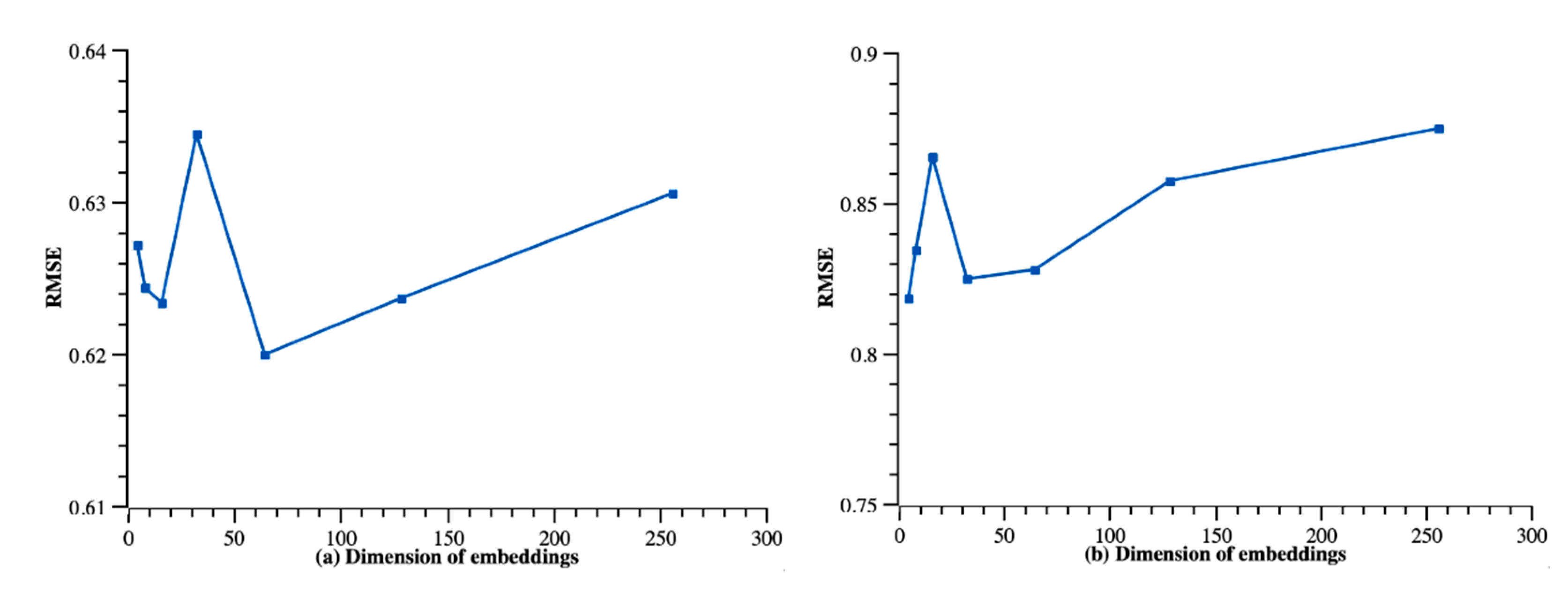
First, in Section 3.2, we conducted the experiment on datasets with the training–testing ratio 90–10% to find the appropriate dimension for embedding vectors. For the movie dataset, as shown in Figure 7a, the lowest RMSE occurred when the dimension of embedding vectors was between 50 and 100, which does not depend on the experimental algorithm to be evaluated. Meanwhile, considering the number of dimensions of a movie’s own attributes, such as classes, user preferences and so on, we chose 64 to be the embedding’s dimension for movies. Similarly, as shown in Figure 7b, we chose 32 to be the embedding vector’s dimension for music.
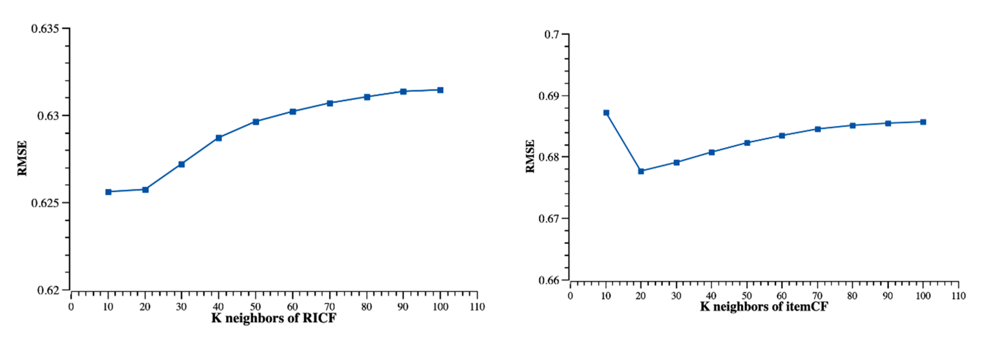
Moreover, the second experiment was conducted to discuss the selection of K-neighbors for RICF. The effects of K-neighbors in RICF are compared with that in traditional itemCF, and the experiment results are shown in Figure 8. We found that only a few K-neighbors are required to achieve good results in RICF and we speculate that the reason is related to the embedding model trained to optimize based on the rating target, because embeddings contain the latent information about the requirement of optimal rating-prediction, so that the more similar the neighbor, the greater the contribution to the rating prediction. Thus, this experiment proved that embedding trained using the rating as the optimization target is able to reduce the number of K-neighbors and hence reduce the computation of the collaborative part. Finally, we chose K = 10 (the minimum K value defined in this paper) as the number of neighbors in the RICF algorithm.
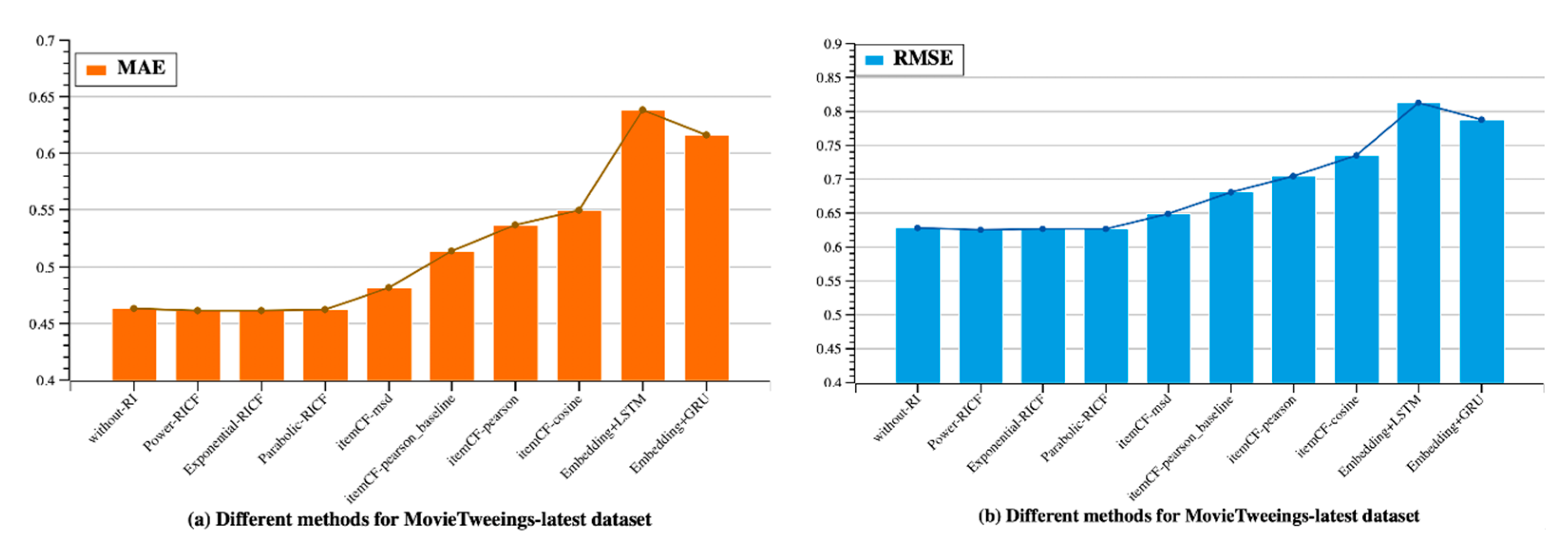
Most notably, this paper investigates the effects of different decay functions in the RICF as well as the comparisons between the traditional itemCF and the state-of-art sequential model that deals with temporal information. In addition, to better explore the process of user preference decay with inhibition, we selected four different ways to model the decay of preferences: (1) without RI effects (without-RI), (2) Power function: obviously decay “quickly then slowly”, (3) Exponential function: no obvious “quickly then slowly”, (4) Parabolic function: as a contrast, it is clear that decay “slowly then quickly”. Finally, the main experiment results on the two datasets are seen in Table 3, Table 4 and Table 5.
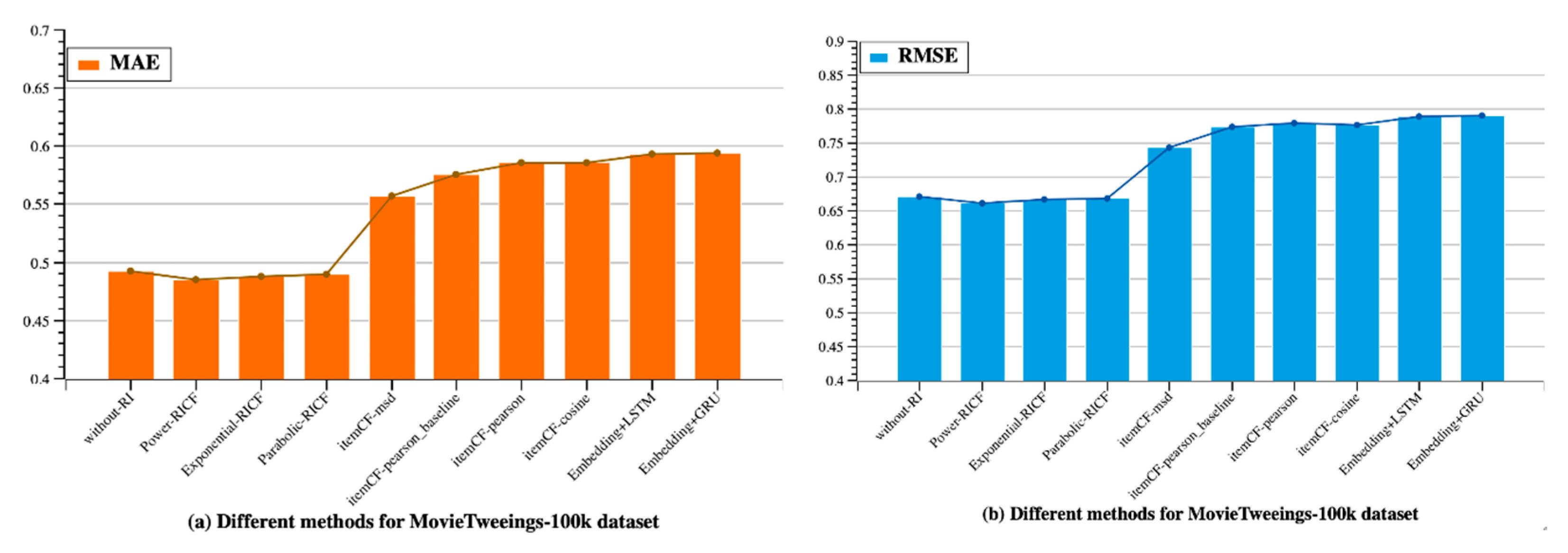
More detailed experiment results are shown in the Figure 9, Figure 10 and Figure 11.
A comprehensive comparison of the Figure 9, Figure 10 and Figure 11 reveals: (1) The RICF algorithm has lower MAE and RMSE than traditional itemCF algorithms, the state-of-art sequential models LSTM and GRU on three datasets used in the experiment. (2) Power-RICF has the lowest MAE and RMSE among the three RICF algorithms. Taking Figure 6 into consideration, the Power function can better fit the process of forgetting in contrast to the Exponential function and Parabolic function, and also it is in tune with the character of preference decay that “first quickly and then slowly”.

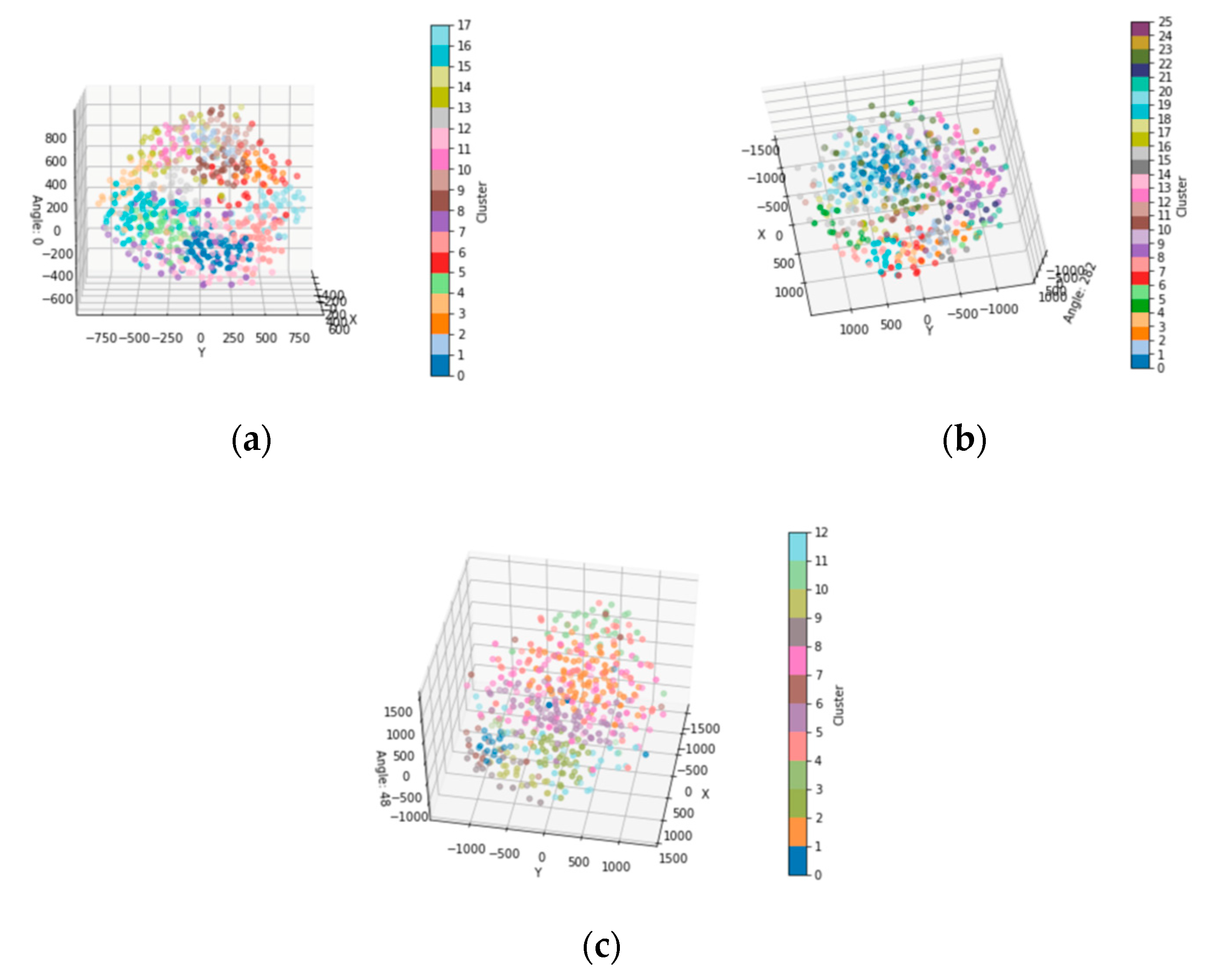
4.3.2. Embedding Clustering Visualization

For the trained multi-dimensional embeddings, we applied t-SNE (t-Distributed Stochastic Neighbor Embedding) to perform dimensional visualization. The t-SNE is a technique for dimensionality reduction that is particularly well suited for the visualization of high-dimensional datasets [54]. According to the previous experiment on the Canopy+K-means algorithm, we clustered the embeddings, as shown in Figure 12, and each color in it represents an embedding cluster. Different clusters represent different user preferences. From the visualization of this figure, we can distinguish the categories of embeddings more clearly. For example, in Figure 12a, the bar on the right shows seventeen colors, representing seventeen different clusters. The coordinate system on the left shows the clustering results in three dimensions. It can be seen that the similar embeddings are clearly clustered, and the boundaries between different clusters are relatively clear.

4.3.3. The stability of RICF

Furthermore, to verify the stability of the RICF algorithm, we separately experimented on three datasets and at the same time, varied the ratio of the training-testing portions from 50% to 90% to observe the results. As can be seen in the Figure 13, Figure 14 and Figure 15, Power-RICF has consistently better performance compared to other experimental algorithms.
As is shown in Figure 13, the x-axis represents different ratios of trainset-testset for MovieTweetings-latest dataset; the y-axis represents the root mean squared error (RMSE) of different algorithms. The left plot shows how the RMSE of the seven different algorithms varies with the ratio of trainset-testset. The plot on the right is a partial enlargement of the plot on the left. As can be seen from Figure 13, the RMSEs of the three RICF algorithms are lower than other algorithms and Power-RICF’s is the lowest. Moreover, for different ratios of trainset-testset, the RMSEs of the RICF algorithms are stable around 0.63, which are the most stable among the seven algorithms.
Figure 14 and Figure 15 show the RMSE of MovieTweetings-100k dataset and DigitalMusic dataset, respectively. Conclusions obtained from Figure 13 and Figure 14 are similar to those from Figure 12. Therefore, for different datasets, the RICF algorithm has better stability and performance than other algorithms, especially Power-RICF.

4.4. Discussion

Currently, there are few studies applying the theory of memory inhibition to Computer Science [11], and studies on Cognitive Psychology have mainly focused on activation propagation, and evolution of preferences from the temporal perspective only, ignoring the competition and inhibition within memories. Thus, in order to fill this gap, we firstly conducted the classical rating-prediction experiment on the traditional itemCF algorithm, and introduced the theory of memory inhibition to explore the evolution of users’ preferences. Secondly, to better take into account the multi-semantic information, we introduced the embedding pre-training technique on the traditional itemCF and used the more efficient Canopy+K-Means algorithm to cluster the multidimensional embeddings to construct the user preference points model, so as to simulate the process of user preference decay and build recommendation models more comprehensively and accurately.
The experiment results show that the memory decay based on retroactive inhibition is consistent with existing memory decay processes (decay first quickly and then slowly) [10,55], and the incorporation of a strong representation of embedding makes the recommendation mechanism more interpretable and has higher prediction accuracy in comparison to traditional itemCF and sequential models. What is more, only fewer neighbors yielded good results when using embeddings to compute similarity and select K neighbors accordingly, unlike traditional CF algorithms that are more reliant on K neighbor selection. Here, the embeddings are trained from a model with rating as an optimization target. We speculate that is because the trained embedding implicitly contains rating-optimized information, which is worthy of further research.
Here, we focused on the problem of rating prediction accuracy of the recommendation algorithm based on retroactive inhibition. We found that in terms of rating prediction accuracy, deep learning-based baseline algorithms perform worse than other baseline algorithms. Similar to most other modern recommendation algorithms, sequence algorithms are not designed for the rating prediction problem, but rather serve to perform the recommendation prediction task better. Therefore, as a future work, we plan to use the proposed algorithm to verify the performance of other recommendation tasks such as prediction ranking.

5. Conclusions

This paper proposed a novel approach called RICF to explore the evolution of user preference based on the theory of retroactive inhibition in cognitive psychology. In RICF, to tackle the problem of data sparsity, each item is represented as a dense numerical vector by training a feedforward deep neural network to predict user preferences for items. Moreover, the Canopy+K-Means clustering algorithm was used to more efficiently cluster multidimensional embedding vectors, and the results of cluster were used to construct a model of users’ points of preference. Evaluation experiments were conducted using three datasets which reflect user’s real rating timestamp (rather than volunteers’ pooled ratings), and the results indicate that the proposed algorithm is better at exploring the evolution of user preference with better accuracy and interpretability. Furthermore, the proposed approach has produced better performance than state-of-the-art techniques on both accuracy and novelty.
Further work consists of three directions. The first direction is to use more sequential datasets to further validate the RICF algorithm. The second direction is to incorporate more diverse information and even the Knowledge Graph technique to train more accurate embedding vectors. The third direction is to explore deeper into the mechanisms of memory inhibition to provide inspiration for sequential modeling algorithms in the field of Deep Learning as well as for the study of other recommendation tasks such as prediction ranking.

Author Contributions

The conceptualization of the original idea, formal analysis, and the performance of the experiment, as well as the original draft preparation, were completed by N.Y. Review and editing were completed by L.C. and Y.Y. All authors have read and agreed to the published version of the manuscript.

Funding

This research was funded by the National Natural Science Foundation of China, grant number 91118002.

Institutional Review Board Statement

Not applicable.

Informed Consent Statement

Not applicable.

Data Availability Statement

Data sharing not applicable. No new data were created or analyzed in this study.

Conflicts of Interest

The authors declare no conflict of interest.

References

  1. Ma, X.; Lu, H.; Gan, Z.; Zeng, J. An Explicit Trust and Distrust Clustering Based Collaborative Filtering Recommendation Approach. Electron. Commer. Res. Appl. 2017, 25, 29–39. [Google Scholar] [CrossRef]
  2. Wang, J.; de Vries, A.P.; Reinders, M.J.T. Unifying User-Based and Item-Based Collaborative Filtering Approaches by Similarity Fusion. In Proceedings of the 29th Annual International ACM SIGIR Conference on Research and Development in Information Retrieval—SIGIR’06, Seattle, WA, USA, 6–11 August 2006; ACM Press: Seattle, WA, USA, 2006; p. 501. [Google Scholar]
  3. Masicampo, E.J.; Ambady, N. Predicting Fluctuations in Widespread Interest: Memory Decay and Goal-Related Memory Accessibility in Internet Search Trends. J. Exp. Psychol. Gener. 2014, 143, 205. [Google Scholar] [CrossRef] [PubMed] [Green Version]
  4. Yin, F.; Su, P.; Li, S.; Ye, L. Step-Enhancement of Memory Retention for User Interest Prediction. IEEE Access 2020, 8, 110203–110213. [Google Scholar] [CrossRef]
  5. Jia, D.; Qu, Z.; Wang, X.; Li, F.; Zhang, L.; Yang, K. Interest Mining Model of Micro-Blog Users by Using Multi-Modal Semantics and Interest Decay Model. In Proceedings of the International Conference on Artificial Intelligence and Security, Hohhot, China, 17–20 July 2020; Springer: Singapore, 2020; pp. 478–489. [Google Scholar]
  6. Lalwani, A.; Agrawal, S. What Does Time Tell? Tracing the Forgetting Curve Using Deep Knowledge Tracing. In Proceedings of the International Conference on Artificial Intelligence in Education, Chicago, IL, USA, 25–29 June 2019; Springer: Cham, Switzerland, 2019; pp. 158–162. [Google Scholar]
  7. Chen, J.; Wang, C.; Wang, J. Modeling the Interest-Forgetting Curve for Music Recommendation. In Proceedings of the ACM International Conference on Multimedia—MM’14, Orlando, FL, USA, 3–7 November 2014; ACM Press: Orlando, FL, USA, 2014; pp. 921–924. [Google Scholar]
  8. Li, T.; Jin, L.; Wu, Z.; Chen, Y. Combined Recommendation Algorithm Based on Improved Similarity and Forgetting Curve. Information 2019, 10, 130. [Google Scholar] [CrossRef] [Green Version]
  9. Yu, H.; Li, Z. A Collaborative Filtering Method Based on the Forgetting Curve. In Proceedings of the 2010 International Conference on Web Information Systems and Mining, Sanya, China, 23–24 October 2010; IEEE: Sanya, China, 2010; pp. 183–187. [Google Scholar]
  10. Walker, M.P.; Brakefield, T.; Hobson, J.A.; Stickgold, R. Dissociable Stages of Human Memory Consolidation and Reconsolidation. Nature 2003, 425, 616–620. [Google Scholar] [CrossRef]
  11. Tempel, T.; Niederée, C.; Jilek, C.; Ceroni, A.; Maus, H.; Runge, Y.; Frings, C. Temporarily Unavailable: Memory Inhibition in Cognitive and Computer Science. Interact. Comput. 2019, 31, 231–249. [Google Scholar] [CrossRef]
  12. Raaijmakers, J.G.W. Inhibition in Memory. In Stevens’ Handbook of Experimental Psychology and Cognitive Neuroscience; Wixted, J.T., Ed.; John Wiley & Sons, Inc.: Hoboken, NJ, USA, 2018; pp. 1–34. ISBN 978-1-119-17016-7. [Google Scholar]
  13. Dooms, S.; De Pessemier, T.; Martens, L. Movietweetings: A Movie Rating Dataset Collected from Twitter. In Proceedings of the Workshop on Crowdsourcing and Human Computation for Recommender Systems, Hong Kong, China, 12–16 October 2013; Volume 2013, p. 43. [Google Scholar]
  14. McAuley, J.; Targett, C.; Shi, Q.; van den Hengel, A. Image-Based Recommendations on Styles and Substitutes. In Proceedings of the 38th International ACM SIGIR Conference on Research and Development in Information Retrieval—SIGIR’15, Santiago, Chile, 9–13 August 2015; ACM Press: Santiago, Chile, 2015; pp. 43–52. [Google Scholar]
  15. Rich, E. User Modeling via Stereotypes. Cognit. Sci. 1979, 3, 329–354. [Google Scholar] [CrossRef]
  16. Salton, G. Automatic Text Processing: The Transformation, Analysis, and Retrieval of Reading; Addison-Wesley: Boston, MA, USA, 1989; Volume 169. [Google Scholar]
  17. Murthi, B.P.S.; Sarkar, S. The Role of the Management Sciences in Research on Personalization. Manag. Sci. 2003, 49, 1344–1362. [Google Scholar] [CrossRef] [Green Version]
  18. Lilien, G.L.; Kotler, P.; Moorthy, K.S. Marketing Models; Prentice Hall: Upper Saddle River, NJ, USA, 1995. [Google Scholar]
  19. Adomavicius, G.; Tuzhilin, A. Toward the next Generation of Recommender Systems: A Survey of the State-of-the-Art and Possible Extensions. IEEE Trans. Knowl. Data Eng. 2005, 17, 734–749. [Google Scholar] [CrossRef]
  20. Breese, J.S.; Heckerman, D.; Kadie, C. Empirical Analysis of Predictive Algorithms for Collaborative Filtering. arXiv 2013, arXiv:1301.7363. [Google Scholar]
  21. Tay, Y.; Anh Tuan, L.; Hui, S.C. Latent Relational Metric Learning via Memory-Based Attention for Collaborative Ranking. In Proceedings of the 2018 World Wide Web Conference, Lyon, France, 23–27 April 2018; pp. 729–739. [Google Scholar]
  22. Yu, K.; Schwaighofer, A.; Tresp, V.; Xu, X.; Kriegel, H.-P. Probabilistic Memory-Based Collaborative Filtering. IEEE Trans. Knowl. Data Eng. 2004, 16, 56–69. [Google Scholar]
  23. Deshpande, M.; Karypis, G. Item-Based Top-n Recommendation Algorithms. ACM Trans. Inf. Syst. (TOIS) 2004, 22, 143–177. [Google Scholar] [CrossRef]
  24. Sarwar, B.; Karypis, G.; Konstan, J.; Reidl, J. Item-Based Collaborative Filtering Recommendation Algorithms. In Proceedings of the Tenth International Conference on World Wide Web—WWW’01, Hong Kong, China, 1–5 May 2001; ACM Press: Hong Kong, China, 2001; pp. 285–295. [Google Scholar]
  25. Aggarwal, C.C. Model-based collaborative filtering. In Recommender Systems; Springer: Cham, Switzerland, 2016; pp. 71–138. [Google Scholar]
  26. Shi, Y.; Larson, M.; Hanjalic, A. List-Wise Learning to Rank with Matrix Factorization for Collaborative Filtering. In Proceedings of the Fourth ACM Conference on Recommender Systems, Barcelona, Spain, 26–30 September 2010; pp. 269–272. [Google Scholar]
  27. Lian, J.; Zhang, F.; Xie, X.; Sun, G. CCCFNet: A Content-Boosted Collaborative Filtering Neural Network for Cross Domain Recommender Systems. In Proceedings of the 26th International Conference on World Wide Web Companion, Perth, Australia, 3–7 April 2017; pp. 817–818. [Google Scholar]
  28. Shi, C.; Hu, B.; Zhao, W.X.; Philip, S.Y. Heterogeneous Information Network Embedding for Recommendation. IEEE Trans. Knowl. Data Eng. 2018, 31, 357–370. [Google Scholar] [CrossRef] [Green Version]
  29. Cai, X.; Han, J.; Yang, L. Generative Adversarial Network Based Heterogeneous Bibliographic Network Representation for Personalized Citation Recommendation. In Proceedings of the AAAI, New Orleans, LA, USA, 2–7 February 2018. [Google Scholar]
  30. Wang, X.; He, X.; Cao, Y.; Liu, M.; Chua, T.-S. Kgat: Knowledge Graph Attention Network for Recommendation. In Proceedings of the 25th ACM SIGKDD International Conference on Knowledge Discovery & Data Mining, Anchorage, AK, USA, 3–7 August 2019; pp. 950–958. [Google Scholar]
  31. Khoshneshin, M.; Street, W.N. Collaborative Filtering via Euclidean Embedding. In Proceedings of the Fourth ACM Conference on Recommender Systems—RecSys’10, Barcelona, Spain, 26–30 September 2010; ACM Press: Barcelona, Spain, 2010; p. 87. [Google Scholar]
  32. Aggarwal, C.C. Recommender Systems; Springer: Cham, Switzerland, 2016; Volume 1. [Google Scholar]
  33. Da Costa, A.F.; Manzato, M.G.; Campello, R.J. Group-Based Collaborative Filtering Supported by Multiple Users’ Feedback to Improve Personalized Ranking. In Proceedings of the 22nd Brazilian Symposium on Multimedia and the Web, Teresina, Brazil, 8–11 November 2016; pp. 279–286. [Google Scholar]
  34. Najafabadi, M.K.; Mahrin, M.N.; Chuprat, S.; Sarkan, H.M. Improving the Accuracy of Collaborative Filtering Recommendations Using Clustering and Association Rules Mining on Implicit Data. Comput. Hum. Behav. 2017, 67, 113–128. [Google Scholar] [CrossRef]
  35. Li, Q.; Kim, B.M. Clustering Approach for Hybrid Recommender System. In Proceedings of the IEEE/WIC International Conference on Web Intelligence (WI 2003), Halifax, NS, Canada, 13–17 October 2003; pp. 33–38. [Google Scholar]
  36. Zhang, W.; Du, Y.; Yoshida, T.; Yang, Y. DeepRec: A Deep Neural Network Approach to Recommendation with Item Embedding and Weighted Loss Function. Inf. Sci. 2019, 470, 121–140. [Google Scholar] [CrossRef]
  37. Barkan, O.; Koenigstein, N. ITEM2VEC: Neural Item Embedding for Collaborative Filtering. In Proceedings of the 2016 IEEE 26th International Workshop on Machine Learning for Signal Processing (MLSP), Vietri sul Mare, Italy, 13–16 September 2016; IEEE: Vietri sul Mare, Italy, 2016; pp. 1–6. [Google Scholar]
  38. Chen, Y.-C.; Hui, L.; Thaipisutikul, T. A Collaborative Filtering Recommendation System with Dynamic Time Decay. J. Supercomput. 2020. [Google Scholar] [CrossRef]
  39. Gui, Y.; Tian, X. A Personalized Recommendation Algorithm Considering Recent Changes in Users’ Interests. In Proceedings of the 2nd International Conference on Big Data Research—ICBDR 2018, Weihai, China, 27–29 October 2018; ACM Press: Weihai, China, 2018; pp. 127–132. [Google Scholar]
  40. Wang, S.; Hu, L.; Wang, Y.; Cao, L.; Sheng, Q.Z.; Orgun, M. Sequential Recommender Systems: Challenges, Progress and Prospects. In Proceedings of the Twenty-Eighth International Joint Conference on Artificial Intelligence, Macao, China, 10–16 August 2019; International Joint Conferences on Artificial Intelligence Organization: Macao, China, 2019; pp. 6332–6338. [Google Scholar]
  41. Xingjian, S.H.I.; Chen, Z.; Wang, H.; Yeung, D.-Y.; Wong, W.-K.; Woo, W. Convolutional LSTM Network: A Machine Learning Approach for Precipitation Nowcasting. In Proceedings of the Advances in Neural Information Processing Systems, Montreal, QC, Canada, 7–12 December 2015; pp. 802–810. [Google Scholar]
  42. Wu, C.-Y.; Ahmed, A.; Beutel, A.; Smola, A.J.; Jing, H. Recurrent Recommender Networks. In Proceedings of the Tenth ACM International Conference on Web Search and Data Mining, Cambridge, UK, 6–10 February 2017; pp. 495–503. [Google Scholar]
  43. Zhang, Z.; Robinson, D.; Tepper, J. Detecting Hate Speech on Twitter Using a Convolution-Gru Based Deep Neural Network. In Proceedings of the European Semantic Web Conference, Anissaras, Greece, 3–7 June 2018; Springer: Anissaras, Greece, 2018; pp. 745–760. [Google Scholar]
  44. Underwood, B.J. Interference and Forgetting. Psychol. Rev. 1957, 64, 49. [Google Scholar] [CrossRef]
  45. Alves, M.V.C.; Bueno, O.F.A. Retroactive Interference: Forgetting as an Interruption of Memory Consolidation. Temas Psicol. 2017, 25, 1055–1067. [Google Scholar] [CrossRef]
  46. Melton, A.W.; von Lackum, W.J. Retroactive and Proactive Inhibition in Retention: Evidence for a Two-Factor Theory of Retroactive Inhibition. Am. J. Psychol. 1941, 54, 157. [Google Scholar] [CrossRef]
  47. Řehuuřek, R.; Sojka, P. Gensim—Statistical Semantics in Python. 2011. Available online: https://radimrehurek.com/gensim/ (accessed on 19 June 2020).
  48. McCallum, A.; Nigam, K.; Ungar, L.H. Efficient Clustering of High-Dimensional Data Sets with Application to Reference Matching. In Proceedings of the Sixth ACM SIGKDD International Conference on Knowledge Discovery and Data Mining, Boston, MA, USA, 20–23 August 2000; pp. 169–178. [Google Scholar]
  49. Zhang, G.; Zhang, C.; Zhang, H. Improved K-Means Algorithm Based on Density Canopy. Knowl. Based Syst. 2018, 145, 289–297. [Google Scholar] [CrossRef]
  50. Kumar, A.; Ingle, Y.S.; Pande, A. Canopy Clustering: A Review on Pre-Clustering Approach to K-Means Clustering. Int. J. Innov. Adv. Comput. Sci. 2014, 3, 22–29. [Google Scholar]
  51. Jain, A.K. Data Clustering: 50 Years beyond K-Means. Pattern Recognit. Lett. 2010, 31, 651–666. [Google Scholar] [CrossRef]
  52. Alsabti, K.; Ranka, S.; Singh, V. An Efficient K-Means Clustering Algorithm. Electr. Eng. Comput. Sci. 1997, 43, 1–7. [Google Scholar]
  53. Harper, F.M.; Konstan, J.A. The Movielens Datasets: History and Context. ACM Trans. Interac. Intell. Syst. 2015, 5, 1–19. [Google Scholar] [CrossRef]
  54. van der Maaten, L.; Hinton, G. Visualizing Data Using T-SNE. J. Mach. Learn. Res. 2008, 9, 2579–2605. [Google Scholar]
  55. Candia, C.; Jara-Figueroa, C.; Rodriguez-Sickert, C.; Barabási, A.-L.; Hidalgo, C.A. The Universal Decay of Collective Memory and Attention. Nat. Hum. Behav. 2019, 3, 82–91. [Google Scholar] [CrossRef]
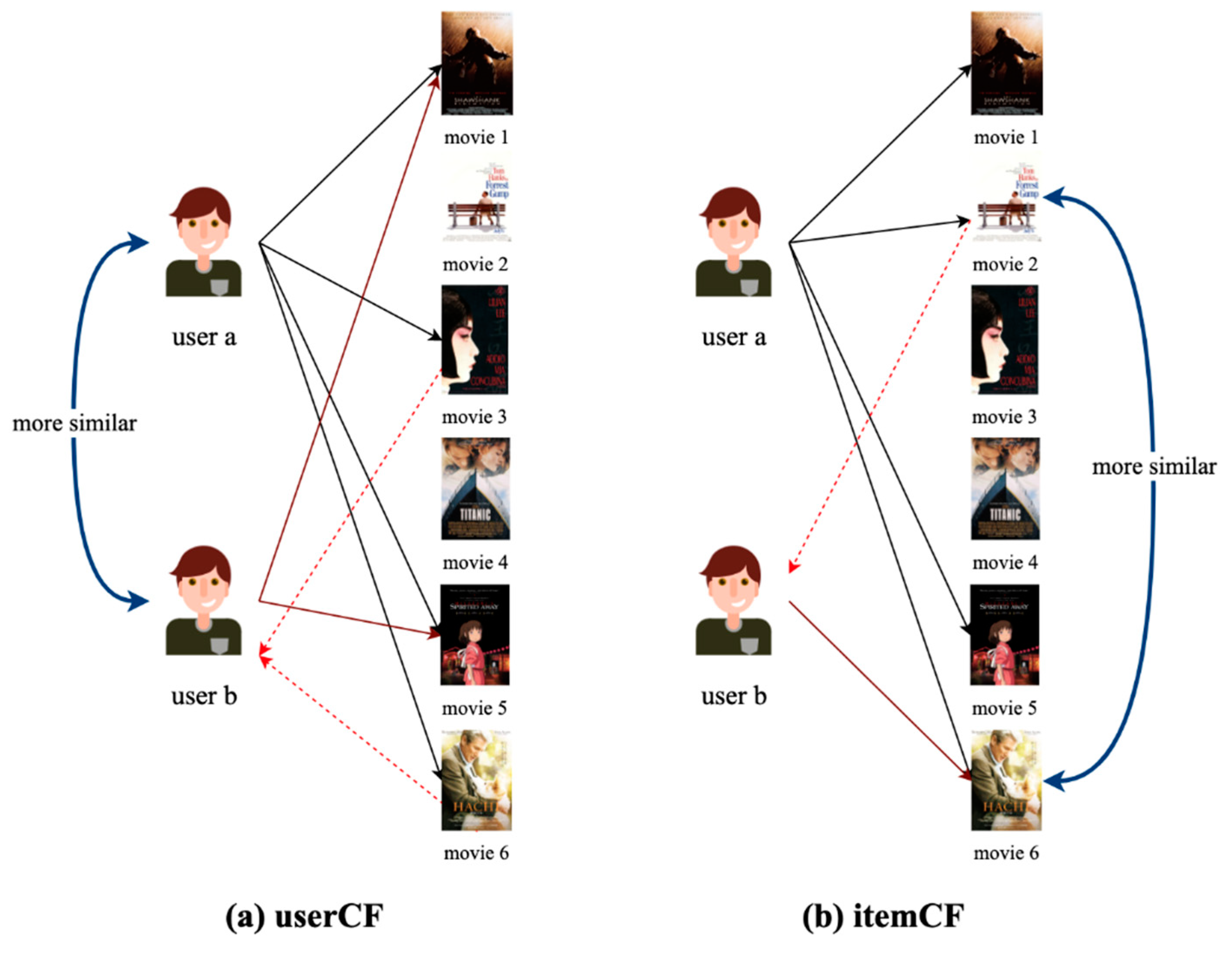
Figure 1. Demonstration for collaborative filtering (CF) algorithms. (a) user-based CF; (b) item-based CF.
Applsci 11 00843 g001
Figure 2. Workflow of proposed algorithm retroactive inhibition of preferences (RICF).
Applsci 11 00843 g002
Figure 3. The description of u i ’s historical preferences.
Applsci 11 00843 g003
Figure 4. (a) The diagram of embedding space; (b) The overall network architecture of the embedding-training model.
Applsci 11 00843 g004
Figure 5. The description of the Canopy+K-Means algorithm, which contains two steps: (a) Canopy pre-clustering (Algorithm 1); (b) K-Means clustering.
Applsci 11 00843 g005
Figure 6. Preferences change over retroactive inhibition (RI)-strength for three different decay functions.
Applsci 11 00843 g006
Figure 7. Root mean squared error (RMSE) of different dimensions of embeddings. (a) Experimental results on MovieTweetings-latest dataset; (b) Experimental results on DigitalMusic dataset.
Applsci 11 00843 g007
Figure 8. RMSE of K-neighbors selection on MovieTweetings-latest dataset.
Applsci 11 00843 g008
Figure 9. The evaluations of ten algorithms for MovieTweetings-latest dataset. (a) mean absolute error (MAE) metric; (b) RMSE metric.
Applsci 11 00843 g009
Figure 10. The evaluations of ten algorithms for MovieTweetings-100k dataset. (a) MAE metric; (b) RMSE metric.
Applsci 11 00843 g010
Figure 11. The evaluations of ten algorithms for DigitalMusic dataset. (a) MAE metric; (b) RMSE metric.
Applsci 11 00843 g011
Figure 12. Visualization of embeddings cluster. (a) Cluster of embeddings in MovieTweetings-latest dataset; (b) cluster of embeddings in MovieTweetings-100k dataset; (c) cluster of embeddings in DigitalMusic dataset.
Applsci 11 00843 g012
Figure 13. RMSE of seven algorithms on the MovieTweetings-latest dataset.
Applsci 11 00843 g013
Figure 14. RMSE of seven algorithms on the MovieTweetings-100k dataset.
Applsci 11 00843 g014
Figure 15. RMSE of seven algorithms on the DigitalMusic dataset.
Applsci 11 00843 g015
Table 1. The structure of sample data.
UserMovieRatingTimePreference ClusterSimilarity to Movie 4
a 12.505 April 2018C10.9
a 34.011 May 2018C20.8
b 43.505 April 2018C31.0
b 12.001 June 2018C10.9
c 22.510 October 2018C40.7
c 33.015 October 2018C20.8
a 4?11 December 2018C31.0
Table 2. The description of datasets.
MovieTweetings-100kMovieTweetings-LatestDigitalMusic
Number of users16,55468,332478,235
Number of items10,50635,931266,414
Number of ratings100,000876,673836,006
Rating range1–101–101–5
Time range28/02/2013 to 01/09/201328/02/2013 to 10/07/202020/01/1998 to 23/07/2014
Table 3. RMSE of different comparative experiments on the MovieTweetings-latest dataset.
RMSEMAE
without-RI0.62720.4624
Power-RICF0.62560.4609
Exponential-RICF0.62600.4614
Parabolic-RICF0.62610.4616
ItemCF0.68090.5134
Embedding+LSTM0.81210.6385
Embedding+GRU0.78700.6158
Table 4. RMSE of different comparative experiments on the MovieTweetings-100k dataset.
RMSEMAE
without-RI0.67110.4919
Power-RICF0.66060.4850
Exponential-RICF0.66630.4877
Parabolic-RICF0.66800.4895
ItemCF0.77410.5752
Embedding+LSTM0.78920.5933
Embedding+GRU0.79080.5935
Table 5. RMSE of different comparative experiments on the DigitalMusic dataset.
RMSEMAE
without-RI0.83890.5971
Power-RICF0.82010.5908
Exponential-RICF0.82980.5923
Parabolic-RICF0.83390.5949
ItemCF0.90790.6277
Embedding+LSTM0.95570.7126
Embedding+GRU0.95080.7106
Publisher’s Note: MDPI stays neutral with regard to jurisdictional claims in published maps and institutional affiliations.