Abstract
Often the input values used in mathematical models for rolling bearings are in a wide range, i.e., very small values of deformation and damping are confronted with big values of stiffness in the governing equations, which leads to miscalculations. This paper presents a two degrees of freedom (2-DOF) dimensionless mathematical model for ball bearings describing a procedure, which helps to scale the problem and reveal the relationships between dimensionless terms and their influence on the system’s response. The derived mathematical model considers nonlinear features as stiffness, damping, and radial internal clearance referring to the Hertzian contact theory. Further, important features are also taken into account including an external load, the eccentricity of the shaft-bearing system, and shape errors on the raceway investigating variable dynamics of the ball bearing. Analysis of obtained responses with Fast Fourier Transform, phase plots, orbit plots, and recurrences provide a rich source of information about the dynamics of the system and it helped to find the transition between the periodic and chaotic response and how it affects the topology of RPs and recurrence quantificators.
1. Introduction
Ball bearings are one of the main components in mechanical systems dealing with transferring the rotational movement and carrying loads, simultaneously assuring high reliability of the structure [1,2]. Years of ball bearings’ development brought the high-precision rolling element bearings in application to a more demanding environment such as space crafts, high-speed rails, or in machines for the semiconductor industry [3], where the reduced friction, vibrations, and heat generation is required. Growing needs and demands require the application of advanced signal processing techniques [4,5] or mathematical description of dynamical phenomena in ball bearings [6,7].
Rotating rolling element bearing generates vibrations related to the parametrical excitation called varying compliance (VC) [8] and characteristic frequencies referring to the specific bearing element [9]. Varying compliance vibrations are related to the number of carrying load rolling elements resulting in rapidly changing stiffness [10,11]. The VC characteristic frequency peak independently from the quality of rolling surfaces or faults and they are related to one of the characteristic ball bearing’s frequencies, i.e., fundamental train frequency (FTF). Other characteristic frequencies refer to the faults of inner ring (BPFI—Ball Passage Frequency Inner), outer ring (BPFO—Ball Passage Frequency Outer), or rolling element (BSF—Ball Spin Frequency) [12,13].
Many internal and external phenomena affect the dynamics of rotational mechanical systems and it is the same in the case of ball bearings. Except for varying compliance vibrations and characteristic frequencies corresponding to the bearing’s design, the following features are the source of nonlinearity in rolling element bearings:
- variable stiffness in time, related to Hertzian contact theory [14,15],
- shape errors and evident faults [16,17],
- friction torque [18],
- radial internal clearance [19],
- subjected external forces [20],
- eccentricity [21],
- thermal expansion influencing the internal geometry [22,23].
In most of the papers related to the mathematical modeling of ball bearings, analyses of response frequencies or statistics-based approaches were proposed to identify faults, while the optimal working conditions and factors inducing vibrations are crucial for future design developments. One of the most important operational parameters is the radial internal clearance denoting the total distance in the radial direction that the inner ring and outer ring can be displaced in relation to each other. The selection of the radial clearance depends on the operating conditions, both too small and too big will result in premature fatigue and short bearing life [24]. Over the years, the influence of the radial clearance was the subject of the research and was discussed by the analysis of the mathematical model and the experiment. Tiwari et al. [25] studied the influence of the radial clearance on the rotor’s dynamics. His analysis brought the information on appearing super- and sub-harmonics in the frequency spectra depending on the clearance value. Tomović et al. [26] found the correlation between the value of radial clearance and the amplitude of vibrations, which has a linear character. Mitrović et al. provided the source of knowledge on radial clearance influence on the ball bearing service life [27] and performed an analysis of grease contamination influence on the RIC by the thermographic inspection [28]. Xu et al. [29] analyzed the bearing response with RMS indicator by variable internal clearance and load.
Based on the above-cited literature, the bearing clearance is a subject of study over the years. However, in most of the papers, the case study bearings with defined parameters in the model are discussed. The alternative is to derive the dimensionless model for a better understanding of terms applied into the mathematical model on each other and characterize the ball bearing dynamic response. The significant increase of the radial clearance during bearing operation is an undesirable phenomenon from the exploitation point of view and it. On its variability, the following factors can have an influence: fitting on the shaft, the thermal expansion, subjected loads, shape errors, and the radial run-out. The first three factors are related to earlier determined operating conditions and they can be more or less predicted. The shape errors in form of roundness or waviness of the rolling surface can be observed in form of numerous and small amplitude frequency peaks. This effect is only measurable during the ball bearing’s assembly process or its disassembly. Another factor is the eccentricity related to the shaft’s manufacturing imperfections, external loads on the rotating shaft, or its improper connection with the motor by the clutch. In our research, we will present the effect of variable eccentricity on the dynamic response of the rolling element bearing.
As the eccentricity introduces additional excitation into the system nonlinearities, such as contact loss in multi-body interactions present in the system play a more important role. Consequently, we expect the appearance of evolution and bifurcations of periodic solutions with the change of the eccentricity. Finally, various instabilities [30] occur in the system. In the specific conditions, chaotic motion [31] can develop, those effects can be studied by different methods [32], such as the Maximal Lyapunov Exponents, Test 0–1 [33] or Multi-Scale Entropy [34]. One of the promising methods to analyze the chaotic response of ball bearings is the recurrence analysis [35,36]. According to Henri Poincaré’s work, the dynamic system comes back to the initial state or its close neighborhood in the phase space after some characteristic time forming so-called Poincaré sections [37]. Eckmann et al. [38] proposed the tool for visualization of the small parts of time series in the form of a recurrence plot (RP), however, to obtain the quantitative information on the considered state, the Recurrence Quantification Analysis has to be conducted [39]. The mentioned method has been already applied to characterize nonlinear dynamics in the variable dynamics of the mechanical systems [40,41,42,43,44] and manufacturing processes [45,46]. The advantage of the recurrence analysis is that it detects the natural behavior of mechanical systems, i.e., occurrence of the same state after some time. That is why, with help of recurrences, it is possible to recognize defects, rapidly changing vibrations as chatters in milling, or varying misalignments or clearance in time. Ball bearings and other rotational systems generate rapidly changing vibrations in time and minor quantitative or qualitative changes in the dynamical response can be studied in short-time intervals. In this paper, it is used for the analysis of ball bearing’s nonlinear dynamics.
The rest of the paper is arranged in the following way. In Section 2, the derived dimensionless mathematical model of rolling-element bearing with its assumptions is discussed. Next, simulation results are presented for different values of eccentricity through FFT, phase plots, and orbit diagrams. In Section 4, the brief theory on the recurrence analysis is presented, and obtained recurrence plots and recurrence quantificators are discussed. Section 5 contains the discussion on results obtained and the next challenges in the mathematical model are mentioned. The last section summarizes the paper.
2. Mathematical Model of the Rolling Element Bearing
2.1. Description of the 2-DOF Mathematical Model of the Rolling Element Bearing
In Figure 1, the ball bearing is presented as the nonlinear spring-damper oscillator with the rotating shaft-inner ring system driven by a constant angular velocity ωs and rigid outer ring. The 2-degrees of freedom (DOF) mathematical model of rolling-element bearing represents the basic operation of the deep groove ball bearings (DGBB) in the x–y plane. In the model, the inner ring and the shaft are treated as one rotating mass and the outer ring is fixed in the housing. The derived mathematical model takes into account external loads that are subjected to the outer ring, the eccentricity of the shaft caused by improper shaft’s coupling or seating, shape errors on the rolling surfaces of the inner and outer ring, variable deformations related to Hertzian contact theory, while the gyroscopic effect is neglected.

Figure 1.
2-degrees of freedom (DOF) mathematical model of the rolling element bearing. The inner ring with the shaft is treated as one rotating mass of the bearing.
In the model, interactions related to the friction torque are neglected, so there are no fluctuations in the angular velocity. The deformation of each rolling element-raceway is taken into account in form of a nonlinear spring. In the DGBB, rolling elements are distributed equally around its circumference with the constant angle ψi, so the angular position of i-th rolling element is calculated from the vertical axis according to the following formula:
where, ψ0 is the angular position of the first ball, i is the angular position of the ball (i = 0, 1, …, n − 1), n is the number of rolling elements, ωc is the rotational velocity of the cage.
The value of the rotational velocity of the cage ωc is determined by the internal geometry of the ball bearing and subjected velocity of the shaft. It is worth emphasizing, that the velocity of the cage is the same as the velocity of each rolling element assuming no slippage.
where, D is the ball diameter, dp is the pitch diameter.
The dimensionless model gives sensitive information on the influence of applied terms on each other [47,48], then the system is scaled and provides the information on the existing dependencies between dimensionless terms and their impact on the system’s dynamics. In the simulation of the derived model, as the global variable, the value of the radial internal clearance is assumed. The mentioned term was taken intentionally, as it has a significant impact on the dynamic response and is related to the variable contact in a ball bearing. In the practical application, the RIC strongly affects the tribology features of ball bearings. In the following subsections, applied nonlinear effects in the mathematical model are discussed.
2.2. Nonlinear Effect—Eccentricity of the Shaft-Inner Ring System
One of the factors affecting the dynamic response of the ball bearing is the eccentricity of the rotor, on which the bearing is seated [49,50]. In rotor-based systems, it is impossible to avoid the shaft’s eccentricity due to its improper manufacturing (mass distribution) or improper coupling with the propelling motor. In the real conditions, the acceptable eccentricity level is equal to (1–6) μm and affects the variable contact in the ball bearing. In Figure 2, the effect of eccentricity acting on the rotor system is presented. The gravitational acceleration (mir + ms)g additionally intensifies the effect of the eccentricity on the system’s dynamics. Centrifugal force Fs of the rotor-bearing system refers to the shifted center of gravity by eccentricity, gravitational acceleration, and deformations in the x–y plane.
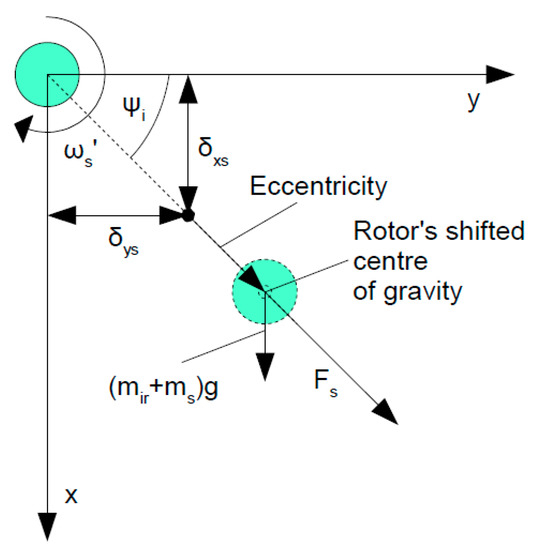
Figure 2.
The graphical representation of the eccentricity of the shaft-inner ring system. The gravity force and subjected loads in the x- and y-axis are acting on the rotating system [10,19].
2.3. Nonlinear Effect—Shape Errors on Rolling Surfaces
As a result of the grinding process, the shape errors (waviness) occur on the rolling surfaces of ball bearings in form of smaller and bigger undulations over the bearing’s circumference. By the fact of rolling over the manufacturing imperfections, additional frequency peaks are induced in a wide range of operational frequencies. The amplitude of frequencies related to the waviness depends on the number of undulations and the value of waves [20,51]. In Figure 3, the graphics showing the visual waviness profile applied in the mathematical model taking into account imperfections on the inner and outer ring. The waviness of balls is omitted as they characterize by smaller values of undulations, the fact is related to the bigger hardness of balls than rings and a longer and more precise manufacturing process (super-finish). Despite the fact that values of respective waves are much smaller than the value of clearance, they should be taken into account during the calculation of nonlinear contact in bearings. As a result of the long-term bearing operation, the depth of each wave propagates and leads to damage. The mathematical description of the raceway waviness for the inner and outer ring is the following:
where Uinner is the amplitude of the inner raceway surface waviness, Ninner is the number of undulations on the inner raceway, Uouter is the amplitude of the outer raceway surface waviness, Nouter is the number of undulations on the outer raceway.
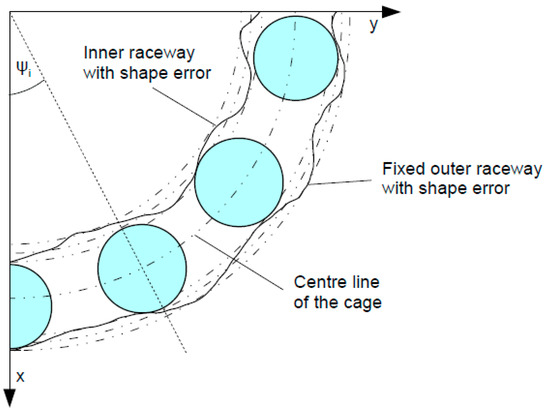
Figure 3.
The graphics presenting the shape error (waviness) on rolling surfaces of the inner and outer ring.
2.4. Nonlinear Effect—Hertzian Contact Theory
Interactions between rolling surfaces in ball bearings are described with the Hertz contact law and its effect has a significant impact on the dynamic response. The shape of the contact in ball bearings depends on the subjected load at most, but the above-mentioned features influence the contact in lesser impact. We can define the elliptical contact in the loaded zone and the point contact in the unloaded zone. Arisen varying deformations result in the nonlinear output of ball bearings and the stronger contact is, the more nonlinear effect is obtained. In the mathematical models of rolling element bearings, the defects of specific elements are also introduced by the variable contact [52,53].
In the derived mathematical model, the elastic contact deformation δi is calculated for each i-th rolling element corresponding to its angular position ψi. In the derived equation (Equation (6)), the effect of radial internal clearance and waviness on rolling surfaces are taken into account:
where δxs, δys are relative displacement between inner and outer rings in the x- and y- directions, respectively. For the δi < 0, there is no contact between rolling surfaces.
Considering the 2-DOF mathematical model, Hertzian contact force [54,55] acts in horizontal (Fy) and vertical (Fx) direction and can be expressed in the following way:
where, kb is the rolling element stiffness, γ is the contact coefficient (point contact in ball bearings γ = 3/2, linear contact in roller bearing γ = 10/9) [56], while H(·) denotes the Heaviside function.
The value of Heaviside, H(·), depends on the contact between rolling surfaces and is formulated as follows:
2.5. Equations of Motion
In the derived mathematical model, the external forces can be subjected in two directions of the x–y plane. Taking into account proposed nonlinear features, the final solution of the mathematical model consists of the following set of differential equations (Equation (10)). The governing equations are obtained by the transformation of the Lagrange equation of 2nd kind taking into consideration the mass of bearing-rotor system equal to 1 for the dimensionless model and they have the following form by defining the state vector [21]:
where (˙) denotes time derivative with respect to the dimensionless time, t, such as t = τΩ (τ is the original time in seconds), Ω is the characteristic frequency scaling the natural frequency related to the linearized continuous contact forces, K′x and K′y: rcγ−1.k′b/m = rcγ−1k′b/m = Ω2. Consequently, ωs = ω′s/Ω. Furthermore, the characteristic lengths and displacements are scaled by the radial clearance rc as the rotor eccentricity ecc = ecc′/rc and corresponding shaft displacements δxs = δ′xs/rc, δys = δ′ys/rc together with their corresponding time derivatives. Dimensionless load force components are Fx—external force subjected in the vertical direction, Fy—external force subjected in the horizontal direction (Fx,y = F′x,y/(m rc Ω2)). While dimensionless damping force components—(cx,y xs,ys) with dimensionless damping coefficients cx,y = c′x,y/Ω.
3. Simulation Results
The derived mathematical model (Equation (10)) is applied in the dimensionless form with Matlab software using ODE 45 (Runge–Kutta method) solver with a relative tolerance of 0.01 and the same value of time step. Dimensionless terms related to the Hertzian contact model are dependent on the global value of the radial internal clearance and the value of the shaft’s eccentricity is taken as the variable parameter. The value of waviness on the rolling surfaces has a weaker impact on the dynamic response and in the real conditions, it can be determined before bearing’s assembly or disassembly process. In Table 1, the values of input parameters (with prime) into the model are specified. To determine the velocity of the cage, the internal geometry (pitch diameter, ball diameter, and the number of balls) is assumed as for the single-row ball bearing 6309. In Table 2, the potential physical parameters are specified corresponding to the dimensionless terms. The system is studied by the internal resonance frequency corresponding the shaft’s angular velocity [57,58]. The dynamic output of the analyzed bearing is taken during its stable operation, i.e., after the starting procedure. It is worth emphasizing, that the load is subjected only to the x-axis (vertical direction) introducing a significant nonlinear effect into the response. The results of the time series, Fast Fourier Transform, phase plots are presented and discussed only from the mentioned direction. In the orbit plots, the results obtained from both axes are taken into account.

Table 1.
Parameters of the rolling element bearing taken for simulation in the dimensionless model, all the lengths are expressed in the clearance value.
Table 2.
Physical parameters corresponding the dimensionless terms.
3.1. Time Series of Deformation and Fast Fourier Transform (FFT)
The bearing-rotor SYSTEM’S dynamic response is examined by the different values of eccentricity as specified in Table 1. The level of the eccentricity is a very common problem in rotational mechanical systems and its too big value, strongly affects the correct operation of the system. In the considered dimensionless model, the value of eccentricity is dependent on the constant clearance value. In Figure 4, the time series of deformation in the x-axis and obtained FFT spectra are presented. In the analyzed model, the ball bearing is radially loaded only in one direction (x-axis) and there is no subjected load in the y-axis, so it is expected to obtain a periodic solution by all considered cases in unloaded direction. As the eccentricity level increases, the response with higher amplitudes is obtained and with stronger nonlinear effects (Figure 4). The effect of stronger nonlinearity in response is observed at FFT spectra, the magnitude of the main harmonic in 1 and its super-harmonics are increasing with the value of eccentricity value up to ecc = 0.35. The main harmonic is marked with the red dashed line in Figure 4 and it corresponds to the frequency of the shaft. Moreover, the increasing value of the eccentricity shows the impact of the waviness on the response by appearing of numerous and small amplitude frequency peaks at FFT spectra.
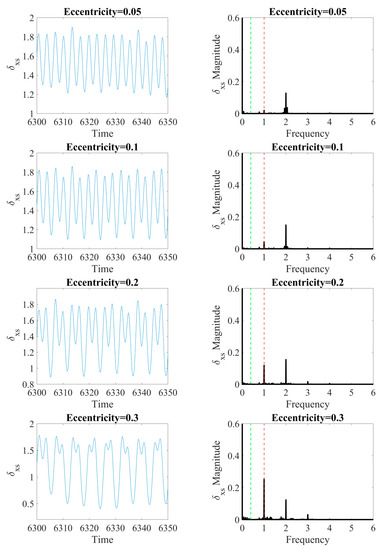
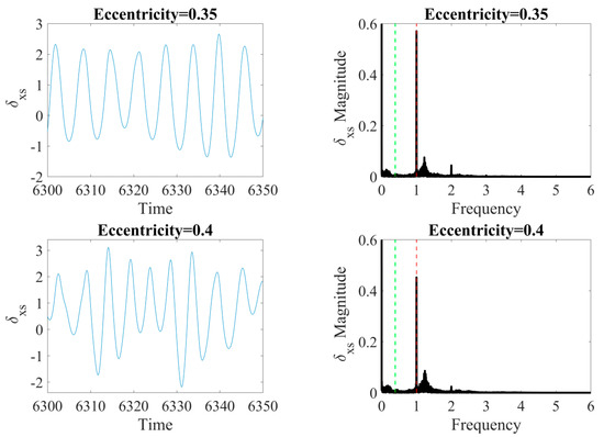
Figure 4.
The time series of deformation in the x-axis (left) and FFT spectra (right) by the different values of the rotor’s eccentricity. In FTT, the red-dashed line corresponds frequency of the shaft’s velocity and the green-dashed line denotes the cage’s characteristic angular frequency.
The increase of eccentricity is affecting the system response with main and higher superharmonics. In the limit of small ecc, we observe the domination of the second harmonic corresponding to parametric excitation with the shaft rotational velocity, ωs. For medium ecc, the peak corresponding to ωs is developing and dominates (see the case with ecc = 0.3). Such interplay of superharmonics in the change of system parameters is common in nonlinear systems. In our case, the parametric excitation is associated with Hertzian stiffness. Note, that in the above-discussed cases with ecc up to 0.3, the δxs is positive which signals that there is no contact loss. Interestingly, for a higher value of eccentricity (see vales ecc = 0.35 and 0.40 in the bottom of Figure 4), we observe the formation of the continuous spectrum of the system response, which could correspond to chaotic behavior. This phenomenon is also typical for nonlinear systems with higher amplitude of excitation, which is controlled by the eccentricity in our system. In these two cases, non-periodic responses are induced additionally by the contact loss which is visible in Figure 4 (see in the left panels for the cases with ecc = 0.35 and 0.40) by the negative values of δxs. Additional frequency peak (frequency at 1.2) in the last two cases could correspond to the variable stiffness with contact loss.
3.2. Orbit Plots and Phase Portraits
For better clarity, for the same values of rotor’s eccentricity, the orbit plots and corresponding δxs-phase plots (Figure 5) are presented to identify and describe the dynamical behavior of the system. As the force is subjected to the x-axis, significant changes are expected in only that direction. Obtained orbit plots for the eccentricity ecc = {0.05; 0.1; 0.2; 0.3} are closed denoting the periodic motion of the bearing. Visible widening of the orbits is presumably related to the additional waviness of the raceway surface.
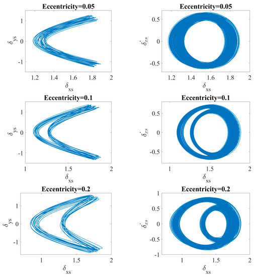
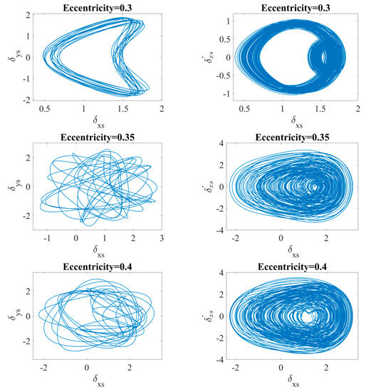
Figure 5.
Orbit plots (left) and phase plots (right) by the different values of the rotor’s eccentricity. Note the contact loss events (δxs crosses negative values for ecc = 0.35 and 0.4).
As the eccentricity is increasing, the deformation in the x-axis is widening creating the moon-shape orbit. The chaotic motion is observed for the eccentricity ecc = {0.35; 0.4}, then the obtained orbit plot has opened structure and the trajectory is not repeatable. Additionally, the temporary contact loss is observed as the 0 value is crossed. The impact of the eccentricity on the dynamical response is also observed at phase plots (Figure 5, right panel), for the periodic solutions the shifting is observed in the x-direction denoting a stronger influence of the nonlinearities. The chaotic solutions have non-regular unstable orbits in his structure as the very similar and close distance trajectories are observed [59]. The application of the basic tools for the diagnostics of dynamical systems allowed us to find the transition between the periodic to chaotic motion. To obtain extended information on the dynamic response of the ball bearing, the advanced nonlinear dynamics methods are applied.
4. Recurrence Analysis
One of the nonlinear dynamics tools, which can be applied for the analysis of ball bearing dynamic response is the recurrence analysis providing the information on all the times when the phase space trajectory of the dynamical system visits roughly the same area in the phase space [60,61]. Then the two points, which are in close distance to each other, are treated as the recurrence points. The distance matrix R (Equation (11)) is for the dynamic state x created with ones (recurrence points) and zeros (no recurrence point) at the times i and j.
where N is the number of considered states, H is the Heaviside function, ε is the threshold distance, is the norm of the dynamic states (for the analysis, the constant recurrence point density norm at recurrence plot was applied RR = 5%).
The recurrence analysis is very popular and widely applied among a variety of sciences such as physiology [62,63], geology [64,65], finances [66,67]. The subject of study is also the diagnostics of the mechanical systems [68,69,70] and recurrences are an alternative method to the standard frequency and time-based methods. In the following subsections, the fundamentals of the recurrence-based methods are presented, i.e., recurrence plots (RP) and Recurrence Quantification Analysis (RQA). The mentioned methods are performed in Matlab software with CRP Toolbox [71].
4.1. Recurrence Plots (RPs) Method
The forerunners of the graphical interpretation of the considered distance matrix [R] are Eckmann et al. [38] and Webber et al. [39], who proposed its analysis in the form of recurrence plots. The mathematical relationship (Equation (12)) describes the formation of the distance matrix with recurrence points and empty spaces (lack of recurrence):
where are the points in the close distance appointed by the threshold radius of ε creating a recurrence point.
Before the recurrence plots can be created, the three parameters must be found beforehand, i.e., time delay—τ, embedding dimension—m, and threshold—ε. According to Takens theorem [72], three mentioned parameters are demanded creating the missing coordinates, then the state of the system after reconstruction can be represented in form of a time-delayed vector [32]:
The first parameter to be found for the phase space reconstruction is the time delay τ for which two methods are specified (a) autocorrelation function and (b) mutual information. The first method is the autocorrelation function [73] given by the following formula:
where, n is the time index of the dynamical process, τ is the time delay, σ2 is the variance of the considered time series. Here the characteristic τ is found to be a decay of cτ reaching 0 or the first minimum.
Another approach for the definition of the time lag is the mutual information function (MI) [74,75]. The method is based on the quantification between the original time series and delayed time series (shifted), the value of time lag τ for the phase space reconstruction is the first minimum. In Figure 6a, the exemplary mutual information function is presented (ecc = 0.4) with the marked first minimum (red-dashed line). The mathematical description of MI has the following form:
where I(x(t),x(t + τ)) is the mutual information function between the original signal and delayed time series, pi, pj are the probability that x(t) is in bin i, j of the histogram constructed from the data points in x, pij(τ) is the probability that x(t) is in bin i and x(t + τ) is in bin j.
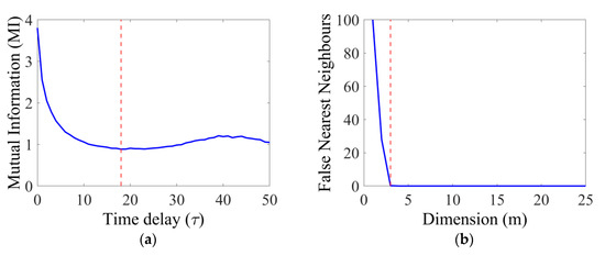
Figure 6.
The mutual information (MI) (a) denotes the time delay (τ) of the phase-space trajectory by the first minimum (red-dashed line). The first minimum of the False Nearest Neighbors (FNN) (b) denotes the dimension (m) in the phase space.
The most popular method of determining the embedding dimension m was proposed by Kennel et al. [76] based on the “False Nearest Neighbors” function. The FNN function detects points in a close distance to each other in the embedding space. The number of embedding dimension m is determined by zero of the FNN function (Figure 6b), then all false neighbors disappear and no further increase of the dimension is necessary [77].
The most demanding step in the phase-space reconstruction is the choice of the threshold ε corresponding to the radius in the phase space. Marwan in his work [35,78] collected a rich source of knowledge on the criteria for its selection, however, the applied method is mostly dependent on the analyzed dynamical system. For our analysis, we assume for the calculation, the method of fixed recurrence rate of 5%. Then the threshold value is adjusted to the density of the recurrence points at RP for all considered cases. This method has two following advantages:
- (1)
- Considered dynamical states are dependent on only one feature at a constant level.
- (2)
- There is no need to normalize considered time series before the phase-space reconstruction.
For analysis of each case, the short time series consisting of 1500 data points was taken for analysis, as the dynamic response is based on the mathematical model and the general character of the deformations is repeatable after the staring procedure. In Table 3, the parameters for the phase space reconstruction are collected, values of a calculated time delay with MI function are on a relatively high level denoting the nonlinear character of the response obtained. The calculated threshold ε is rather on a constant level for 4 cases, taking into account the constant value of the recurrence rate.
Table 3.
The parameters for the reconstruction of recurrence plots (RPs) by the constant value of recurrence rate, RR = 0.05.
By observation of the recurrence plots (Figure 7), it is possible to distinguish periodic and chaotic motion of the ball bearing for specific eccentricity. For small values of the eccentricity, the periodic character of response is observed, confirming the course of the deformation time series (Figure 5a–c). For the eccentricity ecc = 0.3, the periodic character of the response is vanishing, it is evidenced by broken diagonal lines, observance of additional very-short diagonal lines in the perpendicular direction, and single isolated points. The last two cases have a strongly non-regular character with numerous empty zones (indicating losses of correlations) and black regions informing about responses trapped to characteristic states in the corresponding phase space. In those cases, the distances between lines are modulated in unexpected ways informing about multiple unstable orbits that form the chaotic attractor. The square-like structures confirm the presence of intermittences are observed [79,80]. For the last three cases, the stronger influence of vertical structures is visible in contrast to the periodic solutions.
Figure 7.
Recurrence plots for short-time deformation series consisting of 1500 data points for different values of rotor’s eccentricity.
4.2. Recurrence Quantification Analysis (RQA)
As the recurrence plots (RPs) method provides only qualitative information on the system’s dynamics, the quantitative method Recurrence Quantification Analysis (RQA) was proposed in form of recurrence quantificators [81,82]. All the measures are based on the obtain topology of the recurrence plots giving a statistical description of the dynamic output. In this paper, the quantificators determined in the CRP Toolbox [71] are employed and they can be divided by their topology (length and character of diagonal or vertical lines). The recurrence rate is the only quantificator based on the recurrence density.
- Recurrence rate (RR)—informs about the percentage of recurrence points at RPs, for the analysis, the constant RR value was assumed in 5%:
4.2.1. Quantificators Based on the Diagonal Lines
- Determinism (DET)—refers to the percentage of recurrence points producing diagonal lines at the recurrence plot of minimal length μ:
- Average diagonal line length (L)—denotes that a part of the phase-space trajectory is in the close distance during l time steps to another part of the phase-space trajectory in a different time. The L refers to the mean prediction time:
- Length of the longest diagonal line (Lmax)—in contrast to the average diagonal measure, it refers to the length of the longest diagonal (excluding the main diagonal):
- Entropy (ENTR)—is the measure of the distribution of the diagonal segments, it reflects the complexity of the recurrence plot regarding the diagonal lines:
4.2.2. Quantificators Based on the Vertical Lines
- Laminarity (LAM)—refers to the percentage of recurrence points producing vertical lines at the recurrence plot of minimal length μ:
- Trapping time (TT)—denotes the average length of the vertical structures at recurrence plot:
- Length of the longest vertical line (Vmax)—in contrast to the trapping time, this measure refers to the length of the longest vertical:
4.2.3. Quantificators Based on the Recurrence Time
- Recurrence time of the 1st type (T(1))—detects weak transitions in signal dynamics, this quantificator is more robust to the noise level and less sensitive to the parameter change of the algorithm [83]:
- Recurrence time of the 2nd type (T(2))—detects transient states in the signal with very low energy [83]:
4.2.4. Quantificators Based on the Probability
- Recurrence period density entropy (Trec)—quantifies the extent of recurrences [84,85]:
- Clustering coefficient (C)—represents the probability that two recurrences of any state are also neighbors [36,86]:
- Transitivity (ΤRANS)—is the measure allowing to differentiate the periodic or chaotic dynamics [85]:
The bearing’s dynamic response was analyzed with the above-described quantificators, to estimate which of them are sensitive to the variable eccentricity parameter. The results are visualized for the eccentricity ecc = {0; 0.4} with the variable step of 0.05 in Figure 8. The fixed recurrence rate was employed for the calculation of each quantificator to obtain consistent results.
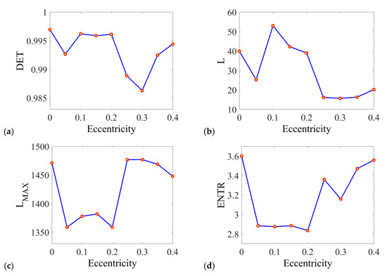
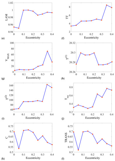
Figure 8.
Results of Recurrence Quantification Analysis (RQA) for the series of rotor’s eccentricity. The analyzed quantificators are following: (a) determinism, (b) averaged diagonal length, (c) length of the longest diagonal, (d) entropy of the diagonal length, (e) laminarity, (f) trapping time, (g) length of the longest vertical line, (h) recurrence time of the 1st type, (i) recurrence time of the 2nd type, (j) recurrence period density entropy, (k) clustering coefficient, (l) transitivity.
The determinism refers to the system’s predictability and its results are convergent with the character of obtained recurrence plots. DET is relatively high (close to 1) for all values of the eccentricity and it slightly decreases with larger eccentricity, then the nonlinear effects influence at most the system’s dynamics.
The average length of the diagonal line gives similar information on the system’s dynamics as the determinism and their trends are very up-close to each other. However, L indicates the stability of periodic intervals reflected in the recurrence plots in a more veritable way, especially it decreases for the high values of the eccentricity when the chaotic dynamics is present from the ecc = 0.25.
Interestingly, the quantificator length of the longest diagonal Lmax has reversed character to the length of the average diagonal L. The divergence of the Lmax values corresponds to the broadening effect of the central diagonal line (see Figure 7). In such a case, L should be more considered as a more reliable indicator of periodic behavior deficiencies.
Entropy provides information on the uncertainty of the bearing’s response. Clearly, the value of entropy is increasing with the increase of the eccentricity. For the periodic solutions, its value is at a constant level.
In the case of the laminarity, it refers to the meantime, when the state of the system is trapped in some states. It also indicates switching between different states of the system. Note, that the laminarity value is close to one in a wide range of eccentricity. As the analyzed mathematical model is deterministic, the transient states can appear only in chaotic response. Consequently, the vertical lines are fairly short, which is also reflected by a small value of the TT parameter.
Trapping time refers to the average length of the vertical lines by the measurement time scale of small changes in the response. The change of TT is convergent with changes observed at recurrence plots, its increasing trend corresponds to the level of the chaotic response of the bearing.
The Vmax has a very similar character to the TT, square-like structures form longer and longer vertical lines with increasing eccentricity. This quantificator strongly reflects obtained structures of RPs.
Recurrence time is mostly used for stochastic signals with numerous transient states, so those measures are not practical for considering the mathematical model. Nevertheless, the recurrence time of the 1st type is very similar to the average length of the diagonal line quantificator L. The recurrence time of the 2nd type has a very similar course to the trapping time, so the vertical line based quantificator.
The Trec has a similar course to the Shannon entropy, this quantificator estimates the average uncertainty of the signal. As for the perfectly periodic signal, the Trec is equal to 0, the periodic and chaotic solutions of the bearing’s response are distinguished.
In the case of clustering coefficient (C) and transitivity (ΤRANS), they have a similar course with minor variability. The constant decrease can be observed from the value of ecc = 0.1, giving information on the increasing influences of nonlinearities on the bearing’s dynamics.
Based on the results presented in Figure 5, we observe that many of the quantificators (including DET, LAM, LMAX, and T(1)) are not very sensitive to the change of the eccentricity. However, the rest of them (including L, ENTR, TT, VMAX, T(2), Trec, C, and TRANS) are changing in some intervals. They could be useful to characterize the system response and consequently to assess the working conditions of the ball bearings.
5. Supplementary Analysis—Kurtosis
One of the statistical quantificators providing the information on the distribution of the results is the kurtosis. With the mentioned parameter, the results obtained of the variable deformation are recalculated for the variable eccentricity output (Figure 9). As the dynamic response has a sinusoidal character, the value of kurtosis for sine and cosine function is close to 1.5 [87]. As the influence of the nonlinear effects increases with the eccentricity, the value of kurtosis is getting bigger within. Kurtosis is increasing linearly till the ecc = 0.25, what is the effect of increasing nonlinearities introduced into the system. The moment when the bearing is getting into the chaotic motion is for the ecc = 0.35, when the value of kurtosis is twice higher than for pure periodic function. When the value kurtosis = 3 or higher, it is the information about the intermittences in the analyzed system [88]. The general character of the kurtosis is similar to the course of recurrence quantificators based on the vertical lines.
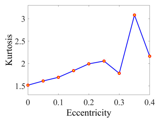
Figure 9.
Kurtosis is calculated for the different values of the rotor’s eccentricity.
6. Results Discussion and Summary
This article reports the results obtained in the analysis of the dimensionless mathematical model for the single-row ball bearing by the recurrence-based methods. For the variable parameter, which is changing the bearing’s dynamics, the shape error in form of the eccentricity was used. The model was studied in a wide range of the operating parameter showing the transition between the periodic and chaotic motion of the system. For studying the behavior of the bearing-shaft system dynamic, the recurrence-based methods were applied in the form of recurrence plots (RPs) and the Recurrence Quantification Analysis (RQA). The analysis aimed to find the transition between the periodic and chaotic response and how does it affect the topology of RPs and recurrence quantificators.
The reconstructed recurrence plots by the constant value of the recurrence rate showed the general character of the system’s dynamics. The periodic solutions are obtained for small values of the eccentricity and they are characterized by the diagonal structure without any disruptions. The square-like structures and isolated recurrence points are evidence of the chaotic motion of the bearing.
The recurrence plots provide only the qualitative information on the system dynamics, so the recurrence quantificators from the Matlab CRP Toolbox were employed for the quantitative analysis. As the mathematical model is studied, the system is deterministic that is proved by the value of DET (Figure 8a). The character of bearing’s response can be roughly determined by the diagonal- (Figure 8b–d) and vertical-based (Figure 8e–g) quantificators, however, the trapping time TT and the length of the longest vertical line Vmax expresses the increasing nonlinearity in the clearest way for interpretation. The recurrence-time of the 2nd type (Figure 8i) has a similar run to TT and Vmax showing clearly the transition between periodic and chaotic motion by the drastic increase of the quantificator. For supplementary analysis, the deformation response was recalculated with the kurtosis. Within its course (Figure 9) the transition between periodic and chaotic solution is identifiable as in the case of vertical line based quantificators.
The performed analysis of the nonlinear mathematical model of the ball bearing showed the usefulness of recurrence-based methods in the identification of its dynamic response. The transition between the periodic and chaotic motion in the variable eccentricity domain was detected with help of recurrence plots and recurrence quantificators. This is evidenced by the square-like structures observed at recurrence plots and radical increase or decrease of recurrence quantificators value in chaotic motion. As many other features are influencing the dynamic response of the ball bearings such as radial clearance or external load, the idea of the mathematical model’s development is to analyze their influence on the system’s dynamics in further steps applying input parameters with assumed uncertainty [89]. Moreover, the model validation is planned by the experimental verification and studying bearing’s response from acceleration measurements.
Author Contributions
Conceptualization, B.A., G.L., A.G. (Anthimos Georgiadis), N.M. and A.G. (Alexander Gassner); methodology, B.A., G.L., A.G. (Anthimos Georgiadis) and N.M.; software, B.A. and G.L.; validation, B.A. and G.L.; formal analysis, B.A., G.L., A.G. (Anthimos Georgiadis), N.M. and A.G. (Alexander Gassner); investigation, B.A. and G.L., resources, B.A., G.L. and A.G. (Anthimos Georgiadis) data curation, B.A. and G.L.; writing—original draft preparation, B.A. and G.L.; writing—review and editing, G.L., A.G. (Anthimos Georgiadis), N.M. and A.G. (Alexander Gassner); visualization, B.A.; supervision, G.L. and A.G. (Anthimos Georgiadis); project administration, B.A., G.L., A.G. (Anthimos Georgiadis) and N.M.; funding acquisition, B.A. and G.L. All authors have read and agreed to the published version of the manuscript.
Funding
The project/research was financed in the framework of the project Lublin University of Technology—Regional Excellence Initiative, funded by the Polish Ministry of Science and Higher Education (contract no. 030/RID/2018/19).
Institutional Review Board Statement
Not applicable.
Informed Consent Statement
Not applicable.
Data Availability Statement
Data available on request due to privacy restrictions.
Conflicts of Interest
The authors declare no conflict of interest.
References
- Cerrada, M.; Sanchez, R.-V.; Li, C.; Pacheco, F.; Cabrera, D.; Valente de Oliveira, J.; Vasquez, R.E. A review on data-driven fault severity assessment in rolling bearings. Mech. Syst. Signal Process. 2018, 99, 169–196. [Google Scholar] [CrossRef]
- Tandon, N.; Choudhury, A. An analytical model for the prediction of the vibration response of rolling element bearings due to a localized defect. J. Sound Vib. 1997, 205, 275–292. [Google Scholar] [CrossRef]
- Wu, D.; Wang, H.; Liu, H.; He, T.; Xie, T. Health monitoring on the spacecraft bearings in high-speed rotating systems by using the clustering fusion of normal acoustic parameters. Appl. Sci. 2019, 9, 3246. [Google Scholar] [CrossRef]
- Huang, D.; Yang, J.; Zhou, D.; Litak, G. Novel adaptive search method for bearing fault frequency using stochastic resonance quantified by amplitude-domain index. IEEE Trans. Instrum. Meas. 2020, 69, 109–121. [Google Scholar] [CrossRef]
- Liu, X.; Liu, H.; Yang, J.; Litak, G.; Cheng, G.; Han, S. Improving the bearing fault diagnosis efficiency by the adaptive stochastic resonance in a new nonlinear system. Mech. Syst. Signal Process. 2017, 96, 58–76. [Google Scholar] [CrossRef]
- Cui, L.; Zhang, Y.; Zhang, F.; Zhang, J.; Lee, S. Vibration response mechanism of faulty outer race rolling element bearings for quantitative analysis. J. Sound Vib. 2016, 364, 67–76. [Google Scholar] [CrossRef]
- Liu, J.; Shao, Y. Overview of dynamic modelling and analysis of rolling element bearings with localized and distributed faults. Nonlinear Dyn. 2018, 93, 1765–1798. [Google Scholar] [CrossRef]
- Tomović, R. A simplified mathematical model for the analysis of varying compliance vibrations of a rolling bearing. Appl. Sci. 2020, 10, 670. [Google Scholar] [CrossRef]
- Hao, Y.; Song, L.; Cui, L.; Wang, H. A three-dimensional geometric features-based SCA algorithm for compound diagnosis. Measurement 2019, 134, 480–491. [Google Scholar] [CrossRef]
- Parmar, V.; Huzur Saran, V.; Harsha, S.P. Effect of an unbalanced rotor on dynamic characteristics of double-row self-aligning ball bearing. Eur. J. Mech. A Solids 2020, 82, 104006. [Google Scholar] [CrossRef]
- Sunnersjö, C.S. Varying compliance vibrations of rolling bearings. J. Sound Vib. 1978, 58, 363–373. [Google Scholar] [CrossRef]
- Ambrożkiewicz, B.; Syta, A.; Meier, N.; Litak, G.; Georgiadis, A. Radial internal clearance analysis in ball bearings. Eksploat. Niezawodn. Maint. Reliab. 2021, 23, 42–54. [Google Scholar] [CrossRef]
- Liu, J.; Xu, Z.; Zhou, L.; Yu, W.; Shao, Y. A statistical feature investigation of the spalling propagation assessment for a ball bearing. Mech. Mach. Theory 2019, 131, 336–350. [Google Scholar] [CrossRef]
- Harris, T.A.; Kotzalas, M.N. Advanced Concepts of Bearing Technology, 5th ed.; CRC Press: Boca Raton, FL, USA, 2007; pp. 41–59. [Google Scholar]
- Liu, J.; Xu, Y.; Wang, L.; Xu, Z.; Tang, C. Influence of local defect distribution on vibration characteristics of ball bearings. Eksploat. Niezawodn. Maint. Reliab. 2019, 21, 485–492. [Google Scholar] [CrossRef]
- Petersen, D.; Howard, C.; Sawalhi, N.; Ahmadi, A.M.; Singh, S. Analysis of bearing stiffness variations, contact forces and vibrations in radially loaded double row rolling element bearings with raceway defects. Mech. Syst. Signal Process. 2015, 50–51, 139–160. [Google Scholar] [CrossRef]
- Kankar, K.; Sharma, S.C.; Harsha, S.P. Vibration based performance prediction of ball bearings caused by localized defects. Nonlinear Dyn. 2012, 69, 847–875. [Google Scholar] [CrossRef]
- Zivkovic, A.; Zeljkovic, M.; Tabakovic, S.; Milojevic, Z. Mathematical modeling and experimental testing of high-speed spindle behavior. Int. J. Adv. Manuf. Technol. 2015, 77, 1071–1086. [Google Scholar] [CrossRef]
- Zhang, Z.; Chen, Y.; Cao, Q. Bifurcations and hysteresis of varying compliance vibrations in the primary parametric resonance for a ball bearing. J. Sound Vib. 2015, 350, 171–184. [Google Scholar] [CrossRef]
- Wang, H.; Han, Q.; Luo, R.; Qing, T. Dynamic modeling of moment wheel assemblies with nonlinear rolling bearing supports. J. Sound Vib. 2017, 406, 124–145. [Google Scholar] [CrossRef]
- Zhuo, Y.; Zhou, X.; Yang, C. Dynamic analysis of double-row self-aligning ball bearings due to applied loads, internal clearance, surface waviness and number of balls. J. Sound Vib. 2014, 333, 6170–6189. [Google Scholar] [CrossRef]
- Gao, S.; Chatterton, S.; Naldi, L.; Pennacchi, P. Ball bearing skidding and over-skidding in large-scale angular contact ball bearings: Nonlinear dynamic model with thermal effects and experimental results. Mech. Syst. Signal Process. 2021, 147, 107120. [Google Scholar] [CrossRef]
- Gao, P.; Chen, Y.; Hou, L. Nonlinear thermal behaviors of the inter-shaft bearing in a dual-rotor system subjected to the dynamic load. Nonlinear Dyn. 2020, 101, 191–209. [Google Scholar] [CrossRef]
- Harsha, S.P. Nonlinear dynamic response of a balanced rotor supported by rolling element bearings due to radial internal clearance. Mech. Mach. Theory 2006, 41, 688–706. [Google Scholar] [CrossRef]
- Tiwari, M.; Gupta, K.; Prakash, O. Dynamic response of an unbalanced rotor supported on ball bearings. J. Sound Vib. 2000, 238, 757–779. [Google Scholar] [CrossRef]
- Tomović, R.; Miltenović, V.; Banić, M.; Miltenović, A. Vibration response of rigid rotor in unloaded rolling element bearing. Int. J. Mech. Sci. 2010, 52, 1176–1185. [Google Scholar] [CrossRef]
- Lazović, T.; Mitrović, R.M.; Ristivojević, M. Influence of internal radial clearance on the ball bearing service life. J. Balk. Tribol. Assoc. 2010, 16, 1–8. [Google Scholar]
- Misković, Z.Z.; Mitrović, R.M.; Stamenić, Z.V. Analysis of grease contamination influence on the internal clearance of ball bearings by thermographic inspection. Therm. Sci. 2016, 20, 255–265. [Google Scholar] [CrossRef]
- Xu, M.; Feng, G.; He, Q.; Gu, F.; Ball, A. Vibration characteristics of rolling element bearings with different radial clearances for condition monitoring of wind turbine. Appl. Sci. 2020, 10, 4731. [Google Scholar] [CrossRef]
- Infante, E.F.; Doughty, S. An old problem reconsidered: The Wahl-Fischer torsional instability problem. J. Appl. Mech. 2020, 87, 101004. [Google Scholar] [CrossRef]
- Bai, C.; Zhang, H.; Xu, Q. Subharmonic resonance of a symmetric ball bearing-rotor system. Int. J. Non-Linear Mech. 2013, 50, 1–10. [Google Scholar] [CrossRef]
- Kantz, H.; Schreiber, T. Nonlinear Time Series Analysis; Cambridge University Press: Cambridge, UK, 2003; pp. 30–47. [Google Scholar]
- Bernardini, D.; Rega, G.; Litak, G.; Syta, A. Identification of regular and chaotic isothermal trajectories of a shape memory oscillator using the 0–1 test. Proc. Inst. Mech. Eng. Part K J. Multi-Body Dyn. 2012, 227, 17–22. [Google Scholar] [CrossRef]
- Brechtl, J.; Xie, X.; Liaw, P.K.; Zinkle, S.J. Complexity modelling and analysis of chaos and other fluctuating phenomena. Chaos Solitions Fractals 2018, 116, 166–175. [Google Scholar] [CrossRef]
- Marwan, N.; Carmen Romano, M.; Thiel, M.; Kurths, J. Recurrence plots for the analysis of complex systems. Phys. Rep. 2007, 438, 237–329. [Google Scholar] [CrossRef]
- Marwan, N.; Donges, J.F.; Zou, Y.; Donner, R.V.; Kurths, J. Complex network approach for recurrence analysis of time series. Phys. Lett. Sect. A Gen. At. Solid State Phys. 2009, 373, 4246–4254. [Google Scholar] [CrossRef]
- Poincaré, H. Sur la probleme des trois corps et les équations de la dynamique. Acta Math. 1890, 13, 1–271. [Google Scholar]
- Eckmann, J.P.; Kamphorst, S.O.; Ruelle, D. Recurrence Plots of Dynamical Systems. Europhys. Lett. 1987, 4, 973–977. [Google Scholar] [CrossRef]
- Zbilut, J.P.; Giuliani, A.; Webber, C.L. Recurrence quantification analysis and principal components in the detection of short complex signals. Phys. Lett. A 1998, 237, 131–135. [Google Scholar] [CrossRef]
- Kitio Kwuimy, C.A.; Samadani, M.; Nataraj, C. Bifurcation analysis of a nonlinear pendulum using recurrence and statistical methods: Applications to fault diagnostics. Nonlinear Dyn. 2014, 76, 1963–1975. [Google Scholar] [CrossRef]
- Kitio Kwuimy, C.A.; Samadani, M.; Kappaganthu, K.; Nataraj, C. Sequential recurrence analysis of experimental time series of a rotor response with bearing outer race faults. Mech. Mach. Sci. 2015, 23, 683–696. [Google Scholar]
- Ambrożkiewicz, B.; Meier, N.; Guo, Y.; Litak, G.; Georgiadis, A. Recurrence-based diagnostics of rotary systems. IOP Conf. Ser. Mater. Sci. Eng. 2019, 710, 012014. [Google Scholar] [CrossRef]
- Syta, A.; Bernardini, D.; Litak, G.; Savi, M.A.; Jonak, K. A comparison of different approaches to detect the transitions from regular to chaotic motions in SMA oscillator. Meccanica 2020, 55, 1295–1308. [Google Scholar] [CrossRef]
- Bo, L.; Liu, X.; Xu, G. Intelligent diagnostics for bearing faults based on intergrated interaction of nonlinear features. IEEE Trans. Ind. Inform. 2020, 16, 1111–1119. [Google Scholar] [CrossRef]
- Rusinek, R.; Lajmert, P. Chatter detection in milling of carbon fiber-reinforced composites by improved Hilbert-Huang Transform and recurrence quantification analysis. Materials 2020, 13, 4105. [Google Scholar] [CrossRef] [PubMed]
- Litak, G.; Syta, A.; Rusinek, R. Dynamical changes during composite milling: Recurrence and multiscale entropy. Int. J. Adv. Manuf. Technol. 2011, 56, 445–453. [Google Scholar] [CrossRef]
- Hu, Q.; Si, X.-S.; Zhang, Q.-H.; Qin, A.-S. A rotating machinery fault diagnosis method based on multi-scale dimensionless indicators and random forests. Mech. Syst. Signal Process. 2020, 139, 106609. [Google Scholar] [CrossRef]
- Meili, L.; Perazzini, H.; Ferreira, M.C.; Freire, J.T. Analyzing the universality of the dimensionless vibrating number based in the effective moisture diffusivity and its impact on specific energy consumption. Heat Mass Transf. 2020, 56, 1659–1672. [Google Scholar] [CrossRef]
- Wang, H.; Han, Q.; Zhou, D. Nonlinear dynamic modelling of rotor system supported by angular contact ball bearings. Mech. Syst. Signal Process. 2017, 85, 16–40. [Google Scholar] [CrossRef]
- Zhang, X.; Han, Q.; Peng, Z.; Chu, F. A comprehensive dynamic model to investigate the stability problems of the rotor-bearing system due to multiple excitations. Mech. Syst. Signal Process. 2016, 70–71, 1171–1192. [Google Scholar] [CrossRef]
- Adamczak, S.; Zmarzły, P. Influence of raceway waviness on the level of vibration in rolling-element bearings. Bull. Pol. Acad. Sci. 2017, 65, 541–551. [Google Scholar] [CrossRef]
- Mishra, C.; Samantaray, A.K.; Chakraborty, G. Ball bearing defect models: A study of simulated and experimental signatures. J. Sound Vib. 2017, 400, 86–112. [Google Scholar] [CrossRef]
- Cui, L.; Huang, J.; Zhang, F.; Chu, F. HVSRMS localization formula and localization law: Localization diagnosis of a ball bearing outer ring fault. Mech. Syst. Signal Process. 2019, 120, 608–629. [Google Scholar] [CrossRef]
- Zhang, Z.; Sattel, T.; Zhu, Y.; Li, X.; Dong, Y.; Rui, X. Mechanism and characteristics of global varying compliance parametric resonances in a ball bearing. Appl. Sci. 2020, 10, 7849. [Google Scholar] [CrossRef]
- Kong, F.; Huang, W.; Jiang, Y.; Wang, W.; Zhao, X. A vibration model of ball bearings with a localized defect based on Hertzian contact stress distribution. Shock Vib. 2018, 5424875, 1–14. [Google Scholar] [CrossRef]
- Laniado-Jacome, E.; Meneses-Alonso, J.; Diaz-Lopez, V. A study of sliding between rollers and races in a roller bearing with a numerical model for mechanical event simulations. Tribol. Int. 2010, 43, 2175–2182. [Google Scholar] [CrossRef]
- Bai, C.; Zhang, H.; Xu, Q. Effects of axial preload of ball bearing on the nonlinear dynamic characteristics of a rotor-bearing system. Nonlinear Dyn. 2008, 53, 173–190. [Google Scholar] [CrossRef]
- Mevel, B.; Guyader, J.L. Experiments on routes to chaos in ball bearings. J. Sound Vib. 2008, 318, 549–564. [Google Scholar] [CrossRef]
- Kostek, R. Simulation and analysis of vibration of rolling bearing. Key Eng. Mater. 2014, 588, 257–265. [Google Scholar] [CrossRef]
- Iwaniec, J.; Uhl, T.; Staszewski, W.J.; Klepka, A. Detection of changes in cracked aluminium plate determinism by recurrence analysis. Nonlinear Dyn. 2012, 70, 125–140. [Google Scholar] [CrossRef]
- Górski, G.; Litak, G.; Mosdorf, R.; Rysak, A. Two phase flow bifurcation due to turbulence: Transition from slugs to bubbles. Eur. Phys. J. B 2015, 88, 239. [Google Scholar] [CrossRef]
- Iwaniec, J.; Iwaniec, M. Heart work analysis by means of recurrence-based methods. Diagnostyka 2017, 18, 89–96. [Google Scholar]
- Groot, V.P.; Rezaee, N.; Wu, W.; Cameron, J.L.; Fishman, E.K.; Hruban, R.H.; Weiss, M.J.; Zheng, L.; Wolfgang, C.L.; He, J. Patterns, timing and predictors of recurrence following pancreatechtomy for pancreatic ductal adenocarcinoma. Ann. Surg. 2018, 267, 936–945. [Google Scholar] [CrossRef] [PubMed]
- Tamura, T.; Oliver, T.S.N.; Cunningham, A.C.; Woodroofe, C.D. Recurrence of extreme coastal erosion in SE Australia beyond historical timescales inferred from beach ridge morphostratigraphy. Geophys. Res. Lett. 2019, 46, 4705–4714. [Google Scholar] [CrossRef]
- Donner, R.V.; Balasis, G.; Stolbova, V.; Georgiou, M.; Wiedermann, M.; Kurths, J. Recurrence-based quantification of dynamical complexity in the Earth’s Magnetosphere at geospace storm timescales. J. Geophys. Res. Space Phys. 2019, 124, 90–108. [Google Scholar] [CrossRef]
- Jiang, Z.Q.; Wang, G.J.; Canabarro, A.; Podobnik, B.; Xie, C.; Stanley, H.E.; Zhou, W.X. Short term prediction of extreme returns based on the recurrence interval analysis. Quant. Financ. 2018, 18, 353–370. [Google Scholar] [CrossRef]
- Meinecke, A.L.; Handke, L.; Mueller-Frommeyer, L.C.; Kauffeld, S. Capturing non-linear temporally embedded processes in organizations using recurrence quantification analysis. Eur. J. Work Organ. Psychol. 2020, 29, 483–500. [Google Scholar] [CrossRef]
- Syta, A.; Jonak, J.; Jedliński, Ł.; Litak, G. Failure diagnosis of a gear box by recurrences. J. Vib. Acoust. 2012, 134, 041006. [Google Scholar] [CrossRef]
- Ambrożkiewicz, B.; Guo, Y.; Litak, G.; Wolszczak, P. Dynamical response of a planetary gear system with faults using recurrence statistics. In Topics in Nonlinear Mechanics and Physics; Springer: Singapore, 2019; pp. 177–185. [Google Scholar]
- Wang, D.F.; Guo, Y.; Wu, X.; Na, J.; Litak, G. Planetary gearbox fault classification by convolutional neural network and recurrence plot. Appl. Sci. 2020, 10, 932. [Google Scholar] [CrossRef]
- Marwan, N. Cross Recurrence Toolbox for Matlab, Reference Manual, Version 5.22, Release 32.5. 2020. Available online: https://tocsy.pik-potsdam.de/CRPtoolbox/ (accessed on 1 December 2020).
- Takens, F. Detecting strange attractors in turbulence. Lect. Notes Math. 1981, 898, 366–381. [Google Scholar]
- Friswell, M.I.; Litak, G.; Sawicki, J.T. Crack identification in rotating machines with active bearings. In Proceedings of the ISMA, Leuven, Belgium, 20–22 September 2010; pp. 2843–2856. [Google Scholar]
- Wallot, S.; Mønster, D. Calculation of Average Mutual Information (AMI) and False-Nearest Neighbours (FNN) for the estimation of embedding parameters of multidimensional time series in Matlab. Front. Psychol. 2018, 9, 1679. [Google Scholar] [CrossRef] [PubMed]
- Fraser, A.M.; Swinney, H.L. Independent coordinates for strange attractors from mutual information. Phys. Rev. A 1986, 33, 1134. [Google Scholar] [CrossRef]
- Kennel, M.B.; Brown, R.; Abarbanel, H.D.I. Determining embedding dimension for phase-space reconstruction using a geometrical construction. Phys. Rev. A 1992, 45, 3403–3411. [Google Scholar] [CrossRef] [PubMed]
- Lin, J.; Huang, Z.; Wang, Y.; Shen, Z. Selection of proper embedding dimension in phase space reconstruction of speech signals. J. Electron. 2000, 17, 161. [Google Scholar] [CrossRef]
- Marwan, N. How to avoid potential pitfalls in recurrence plot based data analysis. Int. J. Bifurc. Chaos 2010, 21, 1–16. [Google Scholar] [CrossRef]
- Sujith, R.I.; Unni, V.R. Complex system approach to investigate and mitigate thermoacoustic instability in turbulent combustors. Phys. Fluids 2020, 32, 061401. [Google Scholar] [CrossRef]
- Kabiraj, L.; Sujith, R.I. Nonlinear self-excited thermoacoustic oscillations: Intermittency and flame blowout. J. Fluid Mech. 2012, 713, 376–397. [Google Scholar] [CrossRef]
- Trulla, L.L.; Giuliani, A.; Zbilut, J.P.; Webber, C.L. Recurrence quantification analysis of the logistic equation with transients. Phys. Lett. A 1996, 223, 255–260. [Google Scholar] [CrossRef]
- Zbilut, J.P.; Giuliani, A.; Webber, C.L. Detecting deterministic signals in exceptionally noisy environments using cross-recurrence quantification. Phys. Lett. A 1998, 246, 122–128. [Google Scholar] [CrossRef]
- Gao, J.B.; Cao, Y.; Gu, L.; Harris, J.G.; Principe, J.C. Detection of weak transitions in signal dynamics using recurrence time statistics. Phys. Lett. A 2003, 317, 64–72. [Google Scholar] [CrossRef]
- Little, M.A.; McSharry, P.E.; Roberts, S.J.; Costello, D.E.A.; Moroz, I.M. Exploiting nonlinear recurrence and fractal scaling properties for voice disorder detection. Biomed. Eng. Online 2007, 6, 23. [Google Scholar] [CrossRef]
- Marwan, N.; Kurths, J.; Foerster, S. Analysing spatially extended high-dimensional dynamics by recurrence plots. Phys. Lett. A 2015, 379, 894–900. [Google Scholar] [CrossRef]
- Donner, R.V.; Zou, Y.; Donges, J.F.; Marwan, N.; Kurths, J. Recurrence networks—A novel paradigm for nonlinear time series analysis. New J. Phys. 2010, 12, 033025. [Google Scholar] [CrossRef]
- Florencias-Oliveros, O.; Gonzalez-de-la-Rosa, J.J.; Aguera-Perez, A.; Palomares-Salas, J.C. Reliability monitoring based on higher-order statistics: A scalable proposal for smart grid. Energies 2018, 12, 55. [Google Scholar] [CrossRef]
- Sen, A.K.; Litak, G.; Edwards, K.D.; Finney, C.E.A.; Daw, C.S.; Wagner, R.M. Characteristics of cyclic heat release variability in the transition from spark ignition to HCCI in a gasoline engine. Appl. Energy 2011, 88, 1649–1655. [Google Scholar] [CrossRef]
- Fu, C.; Xu, Y.; Yang, Y.; Lu, K.; Gu, F.; Ball, A. Response of an accelerating unbalanced rotating system with both random and interval variables. J. Sound Vib. 2020, 466, 115047. [Google Scholar] [CrossRef]
Publisher’s Note: MDPI stays neutral with regard to jurisdictional claims in published maps and institutional affiliations. |
© 2021 by the authors. Licensee MDPI, Basel, Switzerland. This article is an open access article distributed under the terms and conditions of the Creative Commons Attribution (CC BY) license (http://creativecommons.org/licenses/by/4.0/).