A Local Search Maximum Likelihood Parameter Estimator of Chirp Signal

Abstract

A local search Maximum Likelihood (ML) parameter estimator for mono-component chirp signal in low Signal-to-Noise Ratio (SNR) conditions is proposed in this paper. The approach combines a deep learning denoising method with a two-step parameter estimator. The denoiser utilizes residual learning assisted Denoising Convolutional Neural Network (DnCNN) to recover the structured signal component, which is used to denoise the original observations. Following the denoising step, we employ a coarse parameter estimator, which is based on the Time-Frequency (TF) distribution, to the denoised signal for approximate estimation of parameters. Then around the coarse results, we do a local search by using the ML technique to achieve fine estimation. Numerical results show that the proposed approach outperforms several methods in terms of parameter estimation accuracy and efficiency.

1. Introduction

Chirp signals have a broad range of applications, such as in radar, sonar, communication, and medical imaging [1,2]. Chirp usage and estimation of their parameters, i.e., the initial frequency ${\mathrm{f}}_0$ and chirp rate k, is a significant part in the digital signal processing area [3,4]. The main trends in research on chirp signal parameter estimation are improving estimation accuracy, increasing computational efficiency, and enhancing adaptation to low SNRs [5].

At present, TF analysis is an efficient tool to analyze the behavior of nonstationary signals [3]. From TF distribution we can see which frequencies exist at a given time instant. TF transform, e.g., Short-Time Fourier Transform (STFT) [6] and Wigner-Ville Distribution (WVD) [7,8], can convert signals from one-dimensional time domain to two-dimensional TF domain. The Instantaneous Frequency (IF) of a chirp signal is a linear component with time. So, by using line detection methods, e.g., Radon transform [9,10] and Hough transform [11,12,13], which perform integral along all potential lines in TF domain, convert the task of lines detection into locating the maximum peak in the parameter’s domain after integral. Directly use the TF based methods have been practiced to be effective and practical for detecting and estimating chirp signals. But mostly, the signals we sampled are blurred by noises, only from the TF domain can hardly obtain chirp information, and the methods based on Radon–Wigner Transform (RWT) [8,10] or Wigner–Hough Transform (WHT) [11] have heavy computations.

The other typical parameter estimation method is based on the Fractional Fourier Transform (FrFT) [14,15,16,17,18]. FrFT has gained popularity in recent past finding possible application areas especially in signal processing and optics among other disciplines [19,20]. The FRFT is also shown to correspond to a representation of the signal on an orthonormal basis formed by chirps, which are essentially shifted versions of one another [14]. So, FrFT have a good property of energy concentration for chirp signal on a proper transform order. After the FrFT transform of a chirp signal, we can estimate the parameters by searching the peak position in the FrFT domain. Although FrFT performs very well in chirp signal detection, however, in terms of parameter estimation, it is highly influenced by signal length, sample rate, and searching step size.

It has been proved that the ML estimator [21,22] obtains the best performance for finite data samples and is asymptotically optimal in the sense that it achieves the Cramér–Rao Lower Bound (CRLB) [23,24]. Directly use ML estimator to chirp parameters estimation involves a two-dimensional grid search of compressed likelihood function that is limited by computational consideration for high estimation accuracy.

Another approach to chirp parameter estimation is based on deep learning. Data-driven and deep learning-based methods in the digital signal processing area have been of significant interest in recent years. Xiaolong Chen applies Convolutional Neural Network (CNN) for replacing the Fourier transform and FrFT, uses it for single frequency signal and LFM signal detection and estimation [25], it has proved that the CNN based method can achieve good recognition performance in low SNR conditions. Hanning Su addresses the problem of estimating the parameters of constant-amplitude chirp signals that have single or multiple components and are embedded in noise based on a Complex-Valued Deep Neural Network (CV-DNN) [5]. Simulation results indicate that the CV-DNN outperforms conventional processors. And it is more accurate and faster than the WHT, which will enable real-time signal processing with fewer computational resources. Furthermore, they demonstrate that the CV-DNN shows strong robustness to the changes in modulation parameters and the number of components of a chirp signal. Besides chirp signals, Yuan Jiang proposes a deep learning denoising based approach for line spectral estimation [26], by using CNN to preprocess sinusoidal signals in the time domain and offers a substantial improvement in line spectral estimation. As for denoising, Se Rim Park proposes a CNN method to remove noises from speech signals for enhancing the quality and intelligibility of speech [27], the training date and validation data set are the STFT amplitude spectra of the noisy and clean audio signals respectively and then transform back to the time domain by using inverse STFT with amplitude spectra of CNN output and the phase spectrum of the noisy signal. Deep learning also plays an active role in the field of signal detection and classification. Huyong Jin proposes a CNN-based framework to perform preamble detection for underwater acoustic communications applications [28], which can learn features from the TF spectrum and can give an efficient solution for preamble detection under complicated underwater acoustic communications. For signal classification, Johan Brynolfsson uses WVD instead of the spectrogram as basic input into CNN to classify one-dimensional non-stationary signals and has achieved good performance [29].

Inspired by the above ideas, in this paper, we propose a local search maximum likelihood parameter estimator based on the deep learning denoising approach for chirp parameter estimation in low SNR conditions. As shown in Figure 1, the proposed approach consists of a DnCNN, which is trained to perform denoising for noisy observation chirp signals, and a local search estimator applied on the denoised signals and the observations. We explain how DnCNN is composed and the details of the local search estimator. Numerical results show that the proposed approach can yield a substantial improvement in estimation accuracy and efficiency over the RWT and FrFT. The benefit is attributed to the DnCNN denoiser, which can reshape the signal of observation, leading to a great improvement of SNRs.

2. Deep Learning-Based Denoiser

Driven by the easy access to the large-scale dataset and the advances in deep learning methods, there have been several attempts to handle the denoising problem by deep neural networks [30,31,32,33]. In this section, we present the design of the DnCNN used for denoising and the associated training process.

The overall framework of DnCNN is shown in Figure 2 and Figure 3. We modify the ResNet [34,35] to make it suitable for the reshaped signal image array denoising as shown in Figure 3. Unlike the residual network that uses many residual units (i.e., identity shortcuts), our DnCNN employs three single residual units to predict the latent clean signal. With such a residual learning strategy, the network can be easily trained and help ease optimization [35,36].

Generally, DnCNN has a layer structure that includes an input layer, more hidden layers, and a regression output layer. The input of DnCNN is a real mono-component chirp signal blurred by additive white Gaussian noises. We cut the observation sequences $\mathrm{y}\left(\mathrm{n}\right)$ into equal-length segments at regular intervals and splicing them form lift to right in chronological order to form a two-dimensional image matrix, denoted as ${\mathrm{Y}}^0\in R^{\mathrm{m}\times \mathrm{n}}$. The regression output layer computes the half-mean-squared-error loss for regression problems. The optimization goal of training is to minimize the half-mean-squared-error loss between regression output ${\mathrm{y}}_{\mathrm{i}}^{’}\left(\mathrm{n}\right)$ and the clean labels ${\mathrm{x}}_{\mathrm{i}}\left(\mathrm{n}\right)$, then the loss function for training is shown in Equation (1).

$$\mathrm{loss}=\frac{1}{2}{\displaystyle \sum }_{\mathrm{i}=1}^{\mathrm{M}}{\left({\mathrm{y}}_{\mathrm{i}}^{’}-{\mathrm{x}}_{\mathrm{i}}\right)}^2,$$

(1)

where M is mini-batch size, ${\mathrm{y}}_{\mathrm{i}}^{’}\left(\mathrm{n}\right)\in R^{\mathrm{N}\times 1}$ ${\mathrm{x}}_{\mathrm{i}}\in R^{\mathrm{N}\times 1}$, N is the length of observation. During the training process, we use mini-batch gradient descent with Adam optimization algorithm [37] to evaluate the gradient of the loss function and backpropagate to update DnCNN weights. To effectively remove noises of observation, we need to train the DnCNN with a diverse set of training signals with different parameters and SNR conditions that cover the signal of interest. One important factor in generating the training data is the SNR. As the SNR of the test signal is unknown, DnCNN has to be trained with a range of SNR values.

3. Local Search Maximum Likelihood Parameter Estimator

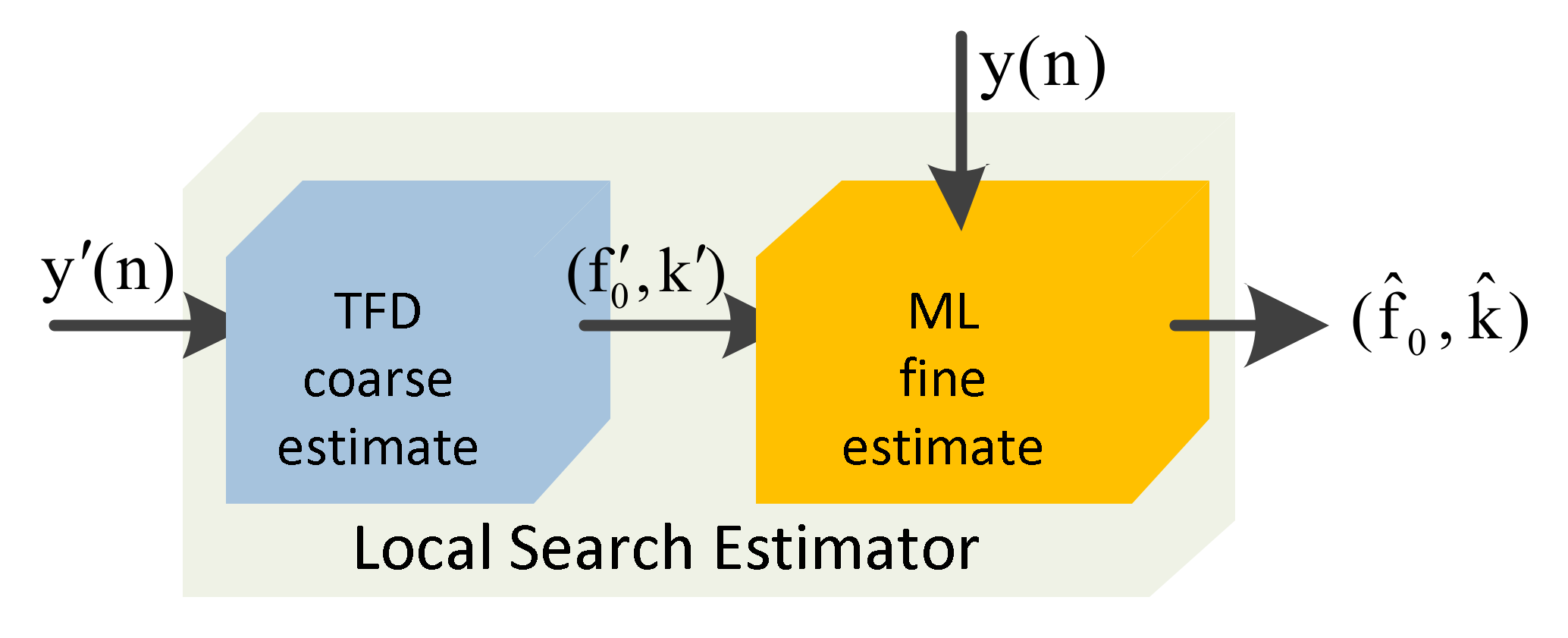
After denoising, parameter estimation is performed by local search estimator using denoised signal ${\mathrm{y}}^{\prime }\left(\mathrm{n}\right)$ and observation $\mathrm{y}\left(\mathrm{n}\right)$. As shown in Figure 4, the proposed approach consists of a TF coarse estimator, which uses TF distribution of ${\mathrm{y}}^{\prime }\left(\mathrm{n}\right)$ to coarsely estimate the initial frequency ${\mathrm{f}}_0^{\prime }$ and chirp rate ${\mathrm{k}}^{\prime }$, then an ML fine estimator applied on the $\left({\mathrm{f}}_0^{\prime },{\mathrm{k}}^{\prime }\right)$ and $\mathrm{y}\left(\mathrm{n}\right)$ to get the fine estimation results of the initial frequency $\widehat{{\mathrm{f}}_0}$ and chirp rate $\hat{\mathrm{k}}$.

3.1. TF Coarse Estimator

A simple and effective parameter estimation method of the chirp signal is to estimate the IF. The IF represents the instantaneous frequency at different time, which combines the initial frequency ${\mathrm{f}}_0^{\prime }$ and chirp rate ${\mathrm{k}}^{\prime }$ in a linear and clear relationship. TF coarse estimator directly uses the IF information of ${\mathrm{y}}^{\prime }\left(\mathrm{n}\right)$. So, its performance is highly influenced by the time-frequency localization and energy concentration about the IF. It is well known that the classical WVD provides a high-resolution TF representation of a mono-component chirp signal [38]. Here we employ WVD for coarse estimation. One important factor that should be noticed in TF coarse estimator is the SNR, since we directly use IF, only when the SNR is high enough, the result is acceptable. We will analyze the improvement of SNR between ${\mathrm{y}}^{\prime }\left(\mathrm{n}\right)$ and $\mathrm{y}\left(\mathrm{n}\right)$ later.

For a discrete signal ${\mathrm{y}}^{\prime }\left(\mathrm{n}\right)$ with N samples, the WVD is defined as Equation (2).

$$\mathrm{WVD}\left(\mathrm{t},\mathrm{f}\right)={\displaystyle \sum }_{\mathrm{m}=-\mathrm{N}}^{\mathrm{N}}{\mathrm{y}}^{\prime }\left(\mathrm{n}+\frac{\mathrm{m}}{2}\right){\mathrm{y}}^{\prime *}\left(\mathrm{n}-\frac{\mathrm{m}}{2}\right){\mathrm{e}}^{-\frac{\mathrm{j}2\mathsf{\pi }\mathrm{km}}{\mathrm{N}}}$$

(2)

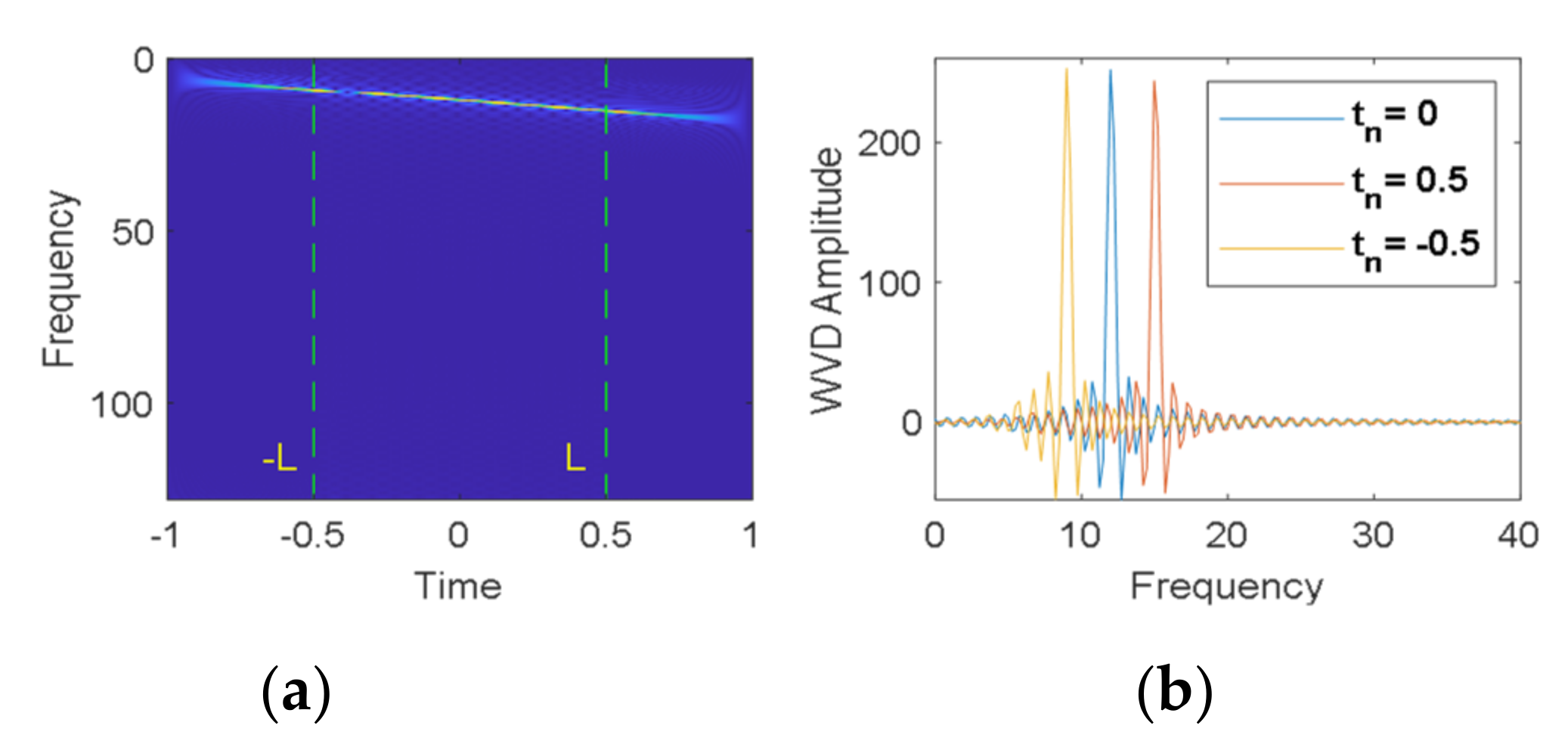
For an ideal chirp signal, its WVD is an impulse spectral line along its IF, finite length chirp signal’s WVD is dorsal fin shape as shown in Figure 5. We can see that the spectrogram of the chirp signal obtains the maximum value at the frequency point ${\mathrm{f}}_0^{\prime }+{\mathrm{k}}^{\prime }\mathrm{t}$ at each discrete time ${\mathrm{t}}_{\mathrm{n}}$. Therefore, the IF of ${\mathrm{y}}^{\prime }\left(\mathrm{n}\right)$ can be estimated by maximizing the spectrogram at each discrete time as Equation (3).

$${\mathrm{f}}_{\mathrm{n}}^{\prime }\left({\mathrm{t}}_{\mathrm{n}}\right)=\underset{{\mathrm{f}}^{\prime }}{\mathrm{argmax}}\left|\mathrm{WVD}\left({\mathrm{t}}_{\mathrm{n}},\mathrm{f}\right)\right|$$

(3)

Considering that there are 2L+1 discrete IF points, then the initial frequency ${\mathrm{f}}_0^{\prime }$ and chirp rate ${\mathrm{k}}^{\prime }$ can be obtained by statistically averaging as Equations (4) and (5).

$${\mathrm{f}}_0^{\prime }=\frac{1}{2\mathrm{L}+1}{\displaystyle \sum }_{\mathrm{n}=-\mathrm{L}}^{\mathrm{n}=\mathrm{L}}{\mathrm{f}}_{\mathrm{n}}^{\prime }\left({\mathrm{t}}_{\mathrm{n}}\right)$$

(4)

$${\mathrm{k}}^{\prime }=\frac{1}{\left({\mathrm{t}}_{\mathrm{L}/2}-{\mathrm{t}}_{-\mathrm{L}/2}\right)\left(\mathrm{L}+1\right)}\left[{\displaystyle \sum }_{\mathrm{n}=0}^{\mathrm{n}=\mathrm{L}}{\mathrm{f}}_{\mathrm{n}}^{\prime }\left({\mathrm{t}}_{\mathrm{n}}\right)-{\displaystyle \sum }_{\mathrm{n}=-\mathrm{L}}^{\mathrm{n}=0}{\mathrm{f}}_{\mathrm{n}}^{\prime }\left({\mathrm{t}}_{\mathrm{n}}\right)\right]$$

(5)

3.2. ML Fine Estimator

After TF coarse estimation, ML fine estimation is performed, the previous result $\left({\mathrm{f}}_0^{\prime },{\mathrm{k}}^{\prime }\right)$ is used to narrow the search scope of the compressed likelihood function of observation $\mathrm{y}\left(\mathrm{n}\right)$. It is worth noting that $\left({\mathrm{f}}_0^{\prime },{\mathrm{k}}^{\prime }\right)$ is estimated by DnCNN’s output ${\mathrm{y}}^{\prime }\left(\mathrm{n}\right)$, however the final estimation results of the ML fine estimator is based on $\mathrm{y}\left(\mathrm{n}\right)$, we will analyze the estimation accuracy of ${\mathrm{y}}^{\prime }\left(\mathrm{n}\right)$ and $\mathrm{y}\left(\mathrm{n}\right)$ later.

Consider an observation $\mathrm{y}\left(\mathrm{n}\right)$ with additive Gaussian white noise, as shown in Equation (6).

$$\mathrm{y}\left(\mathrm{n}\right)=\mathrm{A}\exp \left[\mathrm{j}2\mathsf{\pi }\left({\mathrm{f}}_0\mathrm{n}+\frac{\mathrm{k}}{2}{\mathrm{n}}^2\right)\right]+\mathrm{w}\left(\mathrm{n}\right)$$

(6)

where the parameters, chirp rate $\mathrm{k},$ and initial frequency ${\mathrm{f}}_0$, are unknown. The data model expressed in (10) can be written in matrix form as Equation (7).

$$y=H\mathrm{A}+w$$

(7)

where the signal vector $y$ is given by $y={\left[\mathrm{y}\left(0\right),\dots \mathrm{y}\left(\mathrm{N}-1\right)\right]}^{\mathrm{T}}$, the noise vector $w$ is given by $w={\left[\mathrm{w}\left(0\right),\dots \mathrm{w}\left(\mathrm{N}-1\right)\right]}^{\mathrm{T}}$, ^T denotes the transpose. The matrix $H$ is defined as Equation (8).

$$H=\left[\begin{array}{c}\exp \left(\mathrm{j}2\mathsf{\pi }\left(\mathrm{f}\left(0\right)+\frac{\mathrm{k}}{2}{\left(0\right)}^2\right)\right)\\ ⋮\\ \exp \left(\mathrm{j}2\mathsf{\pi }\left(\mathrm{f}\left(\mathrm{N}-1\right)+\frac{\mathrm{k}}{2}{\left(\mathrm{N}-1\right)}^2\right)\right)\end{array}\right]$$

(8)

Under the ML principle, the ML estimate of $\mathrm{y}\left(\mathrm{n}\right)$ is obtained by maximizing the compressed likelihood function, which describes as Equation (9).

$$\left[\widehat{{\mathrm{f}}_0},\hat{\mathrm{k}}\right]=\underset{\mathrm{f},\mathrm{k}}{\mathrm{argmax}}\left[y^{\mathrm{H}}\left(H{\left[H^{\mathrm{H}}H\right]}^{-1}{H}^{\mathrm{H}}\right)y\right]$$

(9)

^H denotes the conjugate transpose. It can be observed that obtaining ($\widehat{{\mathrm{f}}_0},\hat{\mathrm{k}}$) will require a multidimensional grid search over the two-parameter vectors, which is of high computational load. To avoid that, we resort to the local search method by limit the parameter vectors’ scope to a small area, this operation is based on the result of the TF coarse estimator, which describes as $\mathrm{f}\in \left[{\mathrm{f}}_0{}^{\prime }-{\mathsf{\sigma }}_1,{\mathrm{f}}_0{}^{\prime }+{\mathsf{\sigma }}_1\right]$ and $\mathrm{k}\in \left[{\mathrm{k}}^{\prime }-{\mathsf{\sigma }}_2,{\mathrm{k}}^{\prime }+{\mathsf{\sigma }}_2\right]$, where $\mathsf{\sigma }$ is limitation width. We can see that the accuracy of the TF coarse estimator and the scope of $\mathsf{\sigma }$ directly affect the performance of the proposed estimator, we will analyze it later.

4. Simulation and Analysis

In this section, we present simulation results to demonstrate the performance of the proposed approach for denoising and parameter estimation.

4.1. Training Set and Test Set of DnCNN

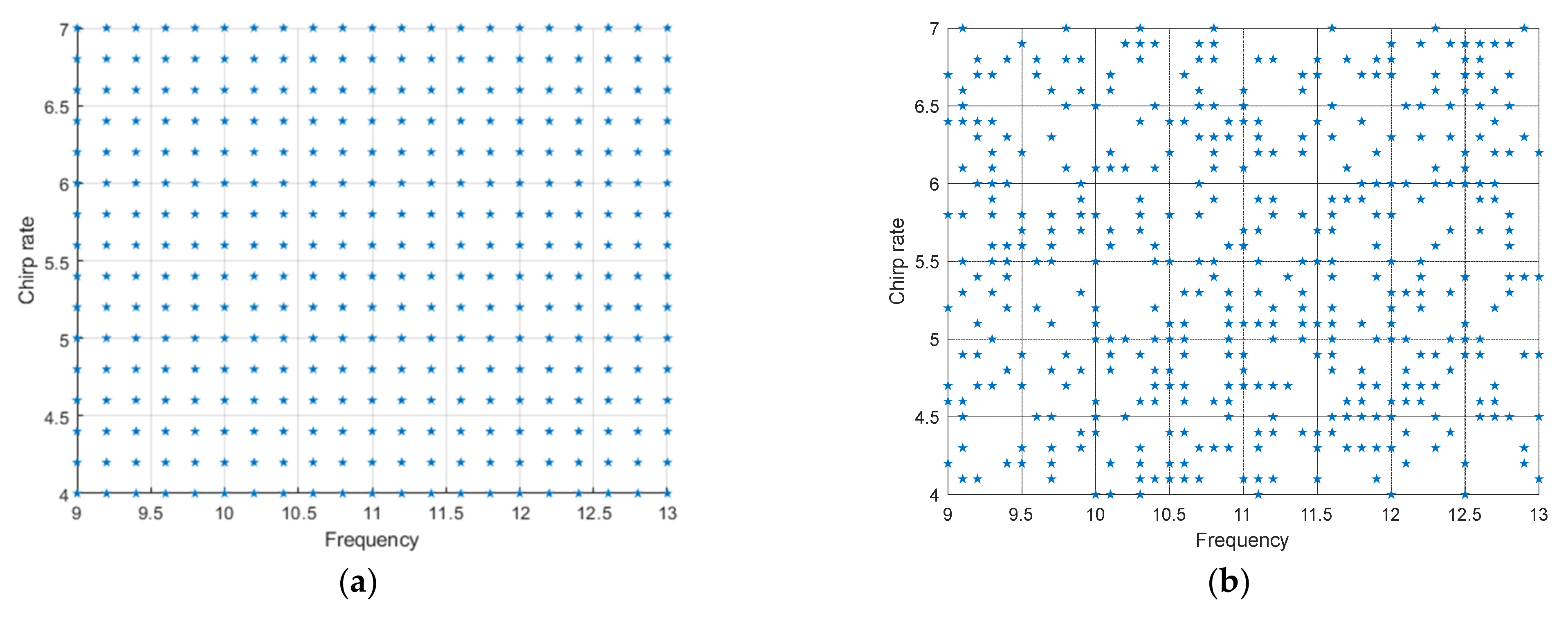
In our simulation, the number of sampling points of the observation $\mathrm{y}\left(\mathrm{n}\right)$ is fixed to N = 513. The midpoint of the signal is the origin of time. The sample frequency is 256. There are only chirp signals and additive white Gaussian noises in the system without other interference or noise. The parameter change scopes of the training set and validation set are ${\mathrm{f}}_0\in \left[9,13\right]$, $\mathrm{k}\in \left[4,7\right]$, and 0.2 as an interval, as shown in Figure 6a. The parameter scope of the test set is the same as the training set, but the parameters are randomly generated, and accurate to one decimal place.

The SNR of the training set varies from –8 dB to –3 dB at an interval of 1dB. We randomly generate ${\mathrm{m}}_{\mathrm{i}}$ signals with the same parameter ${\mathrm{f}}_0$ and k under the specific SNR as shown in

Table 1. Number of ${\mathrm{m}}_{\mathrm{i}}$ in the training set and validation set.

SNR	−8 dB	−7 dB	−6 dB	−5 dB	−4 dB	−3 dB
${\mathrm{m}}_{\mathrm{i}}$ of training Set	150	140	130	120	110	100
${\mathrm{m}}_{\mathrm{i}}$ of validation Set	30	28	26	24	22	20

. The parameter combination has covered all values within the parameter setting range. The validation set size is one-fifth of the training set. For the test set, we randomly generate 500 signals, and SNR varies from –8 dB to 1 dB for each signal as shown in Figure 6b.

In the training process of DnCNN, we set the reshaped signal image array ${\mathrm{Y}}^0\in R^{36\times 57}$. The mini-batch size is 128. The maximum number of the epoch is 4. Before each training epoch, we shuffle the training data. The initial learning rate is 0.0002 and updates the learning rate every epoch by multiplying with the learning rate drop factor 0.9. The training is completed on NVIDIA TITANV GPU with MATLAB Deep Learning Toolbox.

4.2. Numerical Results and Analysis

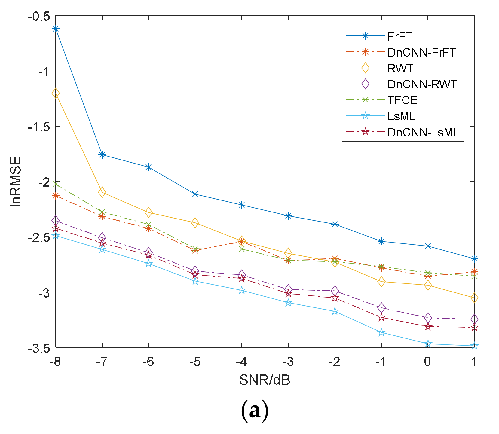
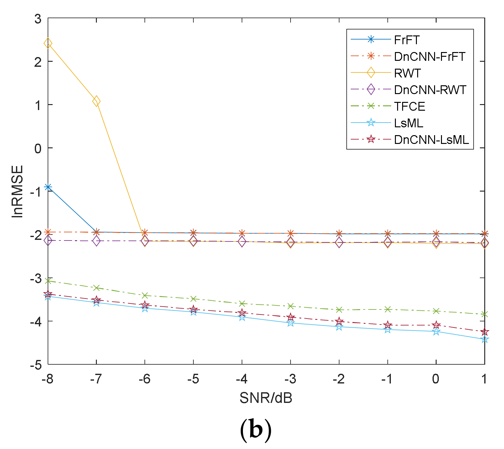
For simplicity, the proposed method is called LsML, TF coarse estimator is called TFCE. The estimator that uses denoised signal ${\mathrm{y}}^{\prime }\left(\mathrm{n}\right)$, as shown in Figure 7, is called DnCNN-XXX. We compare LsML with six other methods including RWT [8] and FrFT [15], which directly use the observation $\mathrm{y}\left(\mathrm{n}\right)$, TFCE, DnCNN-FrFT, DnCNN-RWT and DnCNN-LsML. Figure 8 compare the estimation performance of the above methods in estimating chirp rate $\hat{\mathrm{k}}$ and initial frequency $\widehat{{\mathrm{f}}_0}$. Here, the rotation angle of RWT is from 85 to 91 degrees with an interval of 0.01, the fractional power of FrFT is from 0.96 to 1.08 with an interval of 0.0001, the performance metric is the natural logarithm of Root Mean Squared Error, as described in Equations (10) and (11).

$${\mathrm{lnRMSE}}_{{\mathrm{f}}_0}=\ln (\sqrt{\frac{1}{\mathrm{M}}{\displaystyle \sum }_{\mathrm{i}=1}^{\mathrm{M}}{\left({\mathrm{f}}_{0\mathrm{i}}-{\widehat{{\mathrm{f}}_0}}_{\mathrm{i}}\right)}^2})$$

(10)

$${\mathrm{lnRMSE}}_{\mathrm{k}}=\ln (\sqrt{\frac{1}{\mathrm{M}}{\displaystyle \sum }_{\mathrm{i}=1}^{\mathrm{M}}{({\mathrm{k}}_{\mathrm{i}}-\widehat{{\mathrm{k}}_{\mathrm{i}}})}^2})$$

(11)

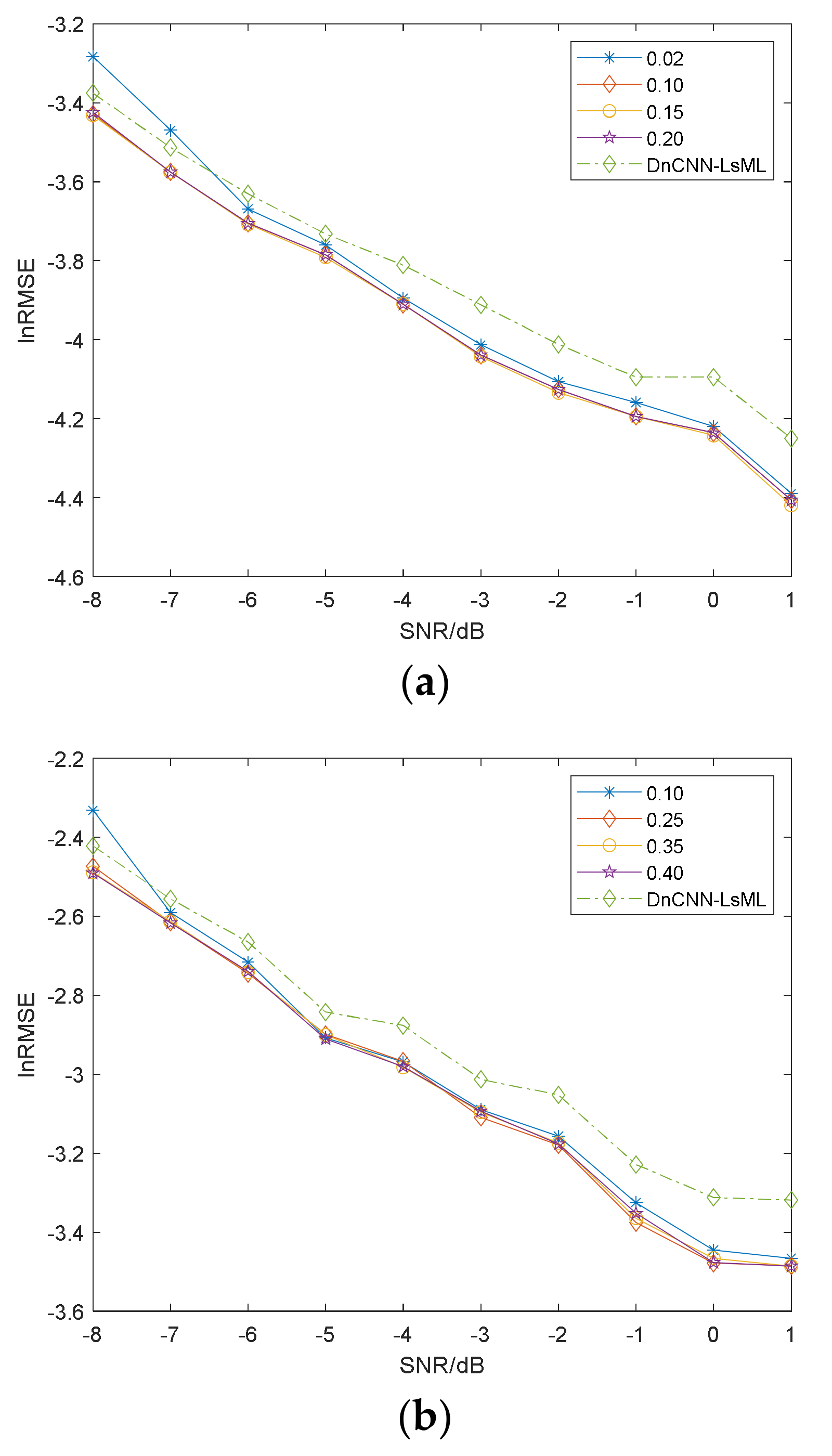
where M = 500 is the number of signals in the test set, ${\mathrm{f}}_{0\mathrm{i}}$ and ${\mathrm{k}}_{\mathrm{i}}$ are the true value, ${\widehat{{\mathrm{f}}_0}}_{\mathrm{i}}$ and $\widehat{{\mathrm{k}}_{\mathrm{i}}}$ are estimation results. The parameter search step of LsML is 0.02, we set the limitation width $\mathsf{\sigma }$ as $\mathrm{f}\in \left[{\mathrm{f}}_0{}^{\prime }-0.15,{\mathrm{f}}_0{}^{\prime }+0.15\right]$ and $\mathrm{k}\in \left[{\mathrm{k}}^{\prime }-0.35,{\mathrm{k}}^{\prime }+0.35\right]$.

Table 2. Average runtime of 100 signals.

Method	RWT	DnCNN-RWT	FrFT	DnCNN-FrFT	TFCE	LsML
Time consumed	0.8925 s	0.9271 s	0.6826 s	0.7464 s	0.0819 s	0.2559 s

lists the average runtime of 100 signals conducted by these methods.

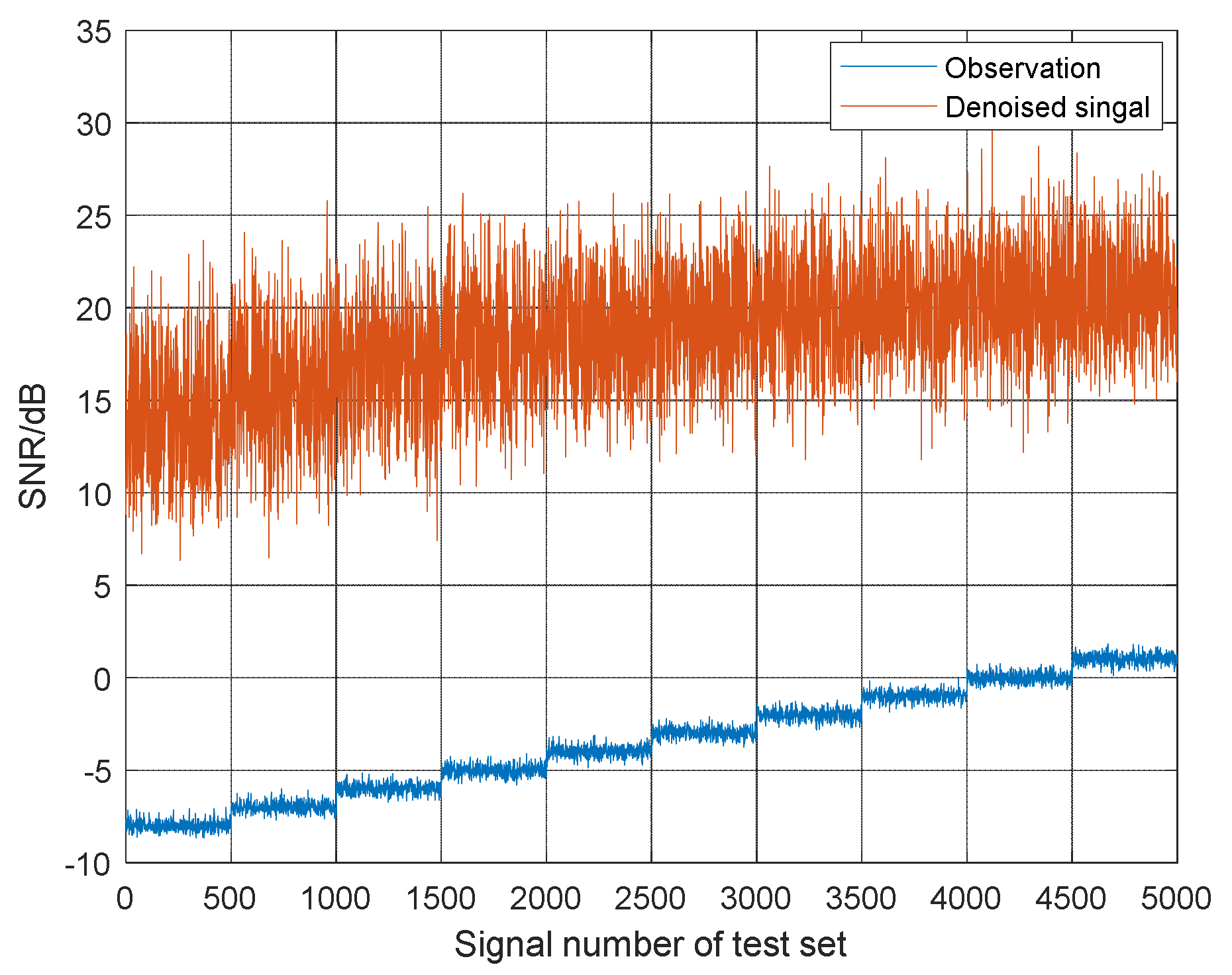
It can be concluded from these results that the proposed LsML has an excellent performance for chirp parameter estimation. By comparing the results of FrFT, RWT, DnCNN-FrFT, and DnCNN-RWT in Figure 8a, we can see that after DnCNN denoising, the accuracy of $\hat{\mathrm{k}}$ is significantly improved. This means that ${\mathrm{y}}^{\prime }\left(\mathrm{n}\right)$ has a higher SNR than $\mathrm{y}\left(\mathrm{n}\right).$ But by comparing the results of LsML and DnCNN-LsML in Figure 8a,b, we can see that observation $\mathrm{y}\left(\mathrm{n}\right)$ is more suitable as input to the ML fine estimator. This means that after denoising of DnCNN, although the SNR of ${\mathrm{y}}^{\prime }\left(\mathrm{n}\right)$ has improved a lot, as shown in Figure 9, the signal parameters have changed slightly. As analyzed before, the accuracy of TFCE determines the value of limitation width $\mathsf{\sigma }$, which will further affect the performance of LsML. The impacts of different $\mathsf{\sigma }$ on estimation accuracy of LsML are shown in Figure 10a,b. We can see that when the SNR is very low, we need a high value of limitation width $\mathsf{\sigma }$.

For generality and comparability, we conducted simulation experiments in the background of additive Gaussian noise. Generally, as long as the spectrum width of noise is much larger than the bandwidth of the system, and the spectral density in this bandwidth can basically be considered as a constant, then we can treat it as white noise. For example, thermal noise and shot noise have uniform power spectral density in a wide frequency range; they can usually be considered as white noise. In specific application scenarios, there are different noise environments. As for the special interference under certain conditions, it needs to be studied separately and explored in-depth, e.g., the Doppler shift and multipath in the field of underwater acoustic engineering. Because the time domain characteristics of the signal have changed a lot, the convolutional network may not be able to extract appropriate features from the training set based on the data labels. The method proposed in the article may not necessarily apply to these interferences.

5. Conclusions

In this paper, three primary ideas are proposed. First, a DnCNN-based method for extracting highly structured chirp signals in low SNR conditions is proposed. It takes advantage of deep learning feature extraction ability to recover the noiseless chirp signals. Second, a TFCE is proposed, we directly use the IF of denoised signal to pre-estimate chirp parameters, which not only have a considerable accuracy but also contribute to improving the performance of ML. Finally, by resorting to the local search method, a non-iterative local searching estimator based on ML is proposed. Simulation results show that the proposed LsML outperforms several methods in terms of parameter estimation accuracy and efficiency in low SNR scenarios.

References

1. Irkhis, L.A.A.; Shaw, A.K. Compressive Chirp Transform for Estimation of Chirp Parameters. In Proceedings of the 2019 27th European Signal Processing Conference (EUSIPCO), A Coruna, Spain, 2–6 September 2019; pp. 1–5. [Google Scholar] [CrossRef]
2. Su, H.; Bao, Q.; Chen, Z. ADMM–Net: A Deep Learning Approach for Parameter Estimation of Chirp Signals Under Sub-Nyquist Sampling. IEEE Access 2020, 8, 75714–75727. [Google Scholar] [CrossRef]
3. Czarnecki, K.; Moszyński, M. A novel method of local chirp-rate estimation of LFM chirp signals in the time-frequency domain. In Proceedings of the 2013 36th International Conference on Telecommunications and Signal Processing (TSP), Rome, Italic, 2–4 July 2013; pp. 704–708. [Google Scholar] [CrossRef]
4. Wang, Y.; Wang, K.; Jing, F.; Lan, X.; Zou, Y.; Wan, L. LFM Signal Analysis Based on Improved Lv Distribution. IEEE Access 2019, 7, 169038–169046. [Google Scholar] [CrossRef]
5. Su, H.; Bao, Q.; Chen, Z. Parameter Estimation Processor for Chirp Signals Based on a Complex-Valued Deep Neural Network. IEEE Access 2019, 7, 176278–176290. [Google Scholar] [CrossRef]
6. Altes, R.A. Detection, estimation, and classification with spectrograms. J. Acoust. Soc. Am. 1980, 67, 1232–1246. [Google Scholar] [CrossRef]
7. Kay, S.; Boudreaux-Bartels, G. On the optimality of the Wigner distribution for detection. In Proceedings of the ICASSP ‘85. IEEE International Conference on Acoustics, Speech, and Signal Processing, Tampa, FL, USA, 26–29 April 1985; Volume 10, pp. 1017–1020. [Google Scholar]
8. Hang, H. Time-Frequency DOA Estimation Based on Radon-Wigner Transform. In Proceedings of the 2006 8th international Conference on Signal Processing, Beijing, China, 16–20 November 2006. [Google Scholar] [CrossRef]
9. Wang, M.; Chan, A.K.; Chui, C.K. Linear frequency-modulated signal detection using Radon-ambiguity transform. IEEE Trans. Signal. Process. 1998, 46, 571–586. [Google Scholar] [CrossRef]
10. Wood, J.C.; Barry, D.T. Radon transformation of time-frequency distributions for analysis of multicomponent signals. IEEE Trans. Signal. Process. 1994, 42, 3166–3177. [Google Scholar] [CrossRef]
11. Barbarossa, S. Analysis of multicomponent LFM signals by a combined Wigner-Hough transform. IEEE Trans. Signal. Process. 1995, 43, 1511–1515. [Google Scholar] [CrossRef]
12. Zhang, X.; Zhang, W.; Yuan, Y.; Cui, K.; Xie, T.; Yuan, N. DOA estimation of spectrally overlapped LFM signals based on Stime-frequencyT and Hough transform. EURASIP J. Adv. Signal. Process. 2019, 2019, 58. [Google Scholar] [CrossRef] [Green Version]
13. Bi, G.; Li, X.; See, C.M.S. LFM signal detection using LPP-Hough transform. Signal. Process. 2011, 91. [Google Scholar] [CrossRef]
14. Almeida, L.B. The fractional Fourier transform and time-frequency representation. IEEE Trans. Signal. Process. 1994, 42, 3084–3091. [Google Scholar] [CrossRef]
15. Ozaktas, H.M.; Arikan, O.; Kutay, M.A.; Bozdagt, G. Digital computation of the fractional Fourier transform. IEEE Trans. Signal. Process. 1996, 44, 2141–2150. [Google Scholar] [CrossRef] [Green Version]
16. Ding, K.; Ding, Q.; Lan, R.Z. Parameters estimation of LFM signal based on fractional order cross spectrum. In Proceedings of the 2011 International Conference on Electronic & Mechanical Engineering and Information Technology, Harbin, China, 12–14 August 2011; pp. 654–656. [Google Scholar] [CrossRef]
17. Narayanan, V.; Prabhu, K.M.M. The fractional Fourier transform: Theory, implementation and error analysis. Microprocess. Microsyst. 2003, 27, 511–521. [Google Scholar] [CrossRef]
18. Ding, Y.; Sun, L.; Zhang, H.; Zheng, B. A multi-component LFM signal parameters estimation method using Stime-frequencyT and Zoom-FRFT. In Proceedings of the 2016 8th IEEE International Conference on Communication Software and Networks (ICCSN), Beijing, China, 4–6 June 2016; pp. 112–117. [Google Scholar] [CrossRef]
19. Ozaktas, H.M.; Zalevski, Z.; Kutay, M.A. The Fractional Fourier Transform with Applications in Optics and Signal Processing; Wiley: Chichester, UK, 2001. [Google Scholar]
20. Akay, O.; Erözden, E. Employing Fractional Autocorrelation for Fast Detection and Sweep Rate Estimation of Pulse Compression Radar Waveforms. Signal. Process. 2009, 89. [Google Scholar] [CrossRef]
21. Abatzoglou, T. Fast maximum likelihood joint estimation of frequency and frequency rate. In Proceedings of the ICASSP ‘86 IEEE International Conference on Acoustics, Speech, and Signal Processing, Tokyo, Japan, 7–11 April 1986; pp. 1409–1412. [Google Scholar] [CrossRef]
22. Saha, S.; Kay, S. A noniterative maximum likelihood parameter estimator of superimposed chirp signals. In Proceedings of the 2001 IEEE International Conference on Acoustics, Speech, and Signal Processing. Proceedings (Cat. No.01CH37221), Salt Lake City, UT, USA, 7–11 May 2001; Volume 5, pp. 3109–3112. [Google Scholar] [CrossRef]
23. Saha, S.; Kay, S.M. Maximum likelihood parameter estimation of superimposed chirps using Monte Carlo importance sampling. IEEE Trans. Signal. Process. 2002, 50, 224–230. [Google Scholar] [CrossRef]
24. Lin, Y.; Peng, Y.; Wang, X. Maximum likelihood parameter estimation of multiple chirp signals by a new Markov chain Monte Carlo approach. In Proceedings of the 2004 IEEE Radar Conference (IEEE Cat. No.04CH37509), Philadelphia, PA, USA, 29 April 2004; pp. 559–562. [Google Scholar] [CrossRef]
25. Chen, X.; Jiang, Q.; Su, N.; Chen, B.; Guan, J. LFM Signal Detection and Estimation Based on Deep Convolutional Neural Network. In Proceedings of the 2019 Asia-Pacific Signal and Information Processing Association Annual Summit and Conference (APSIPA ASC), Lanzhou, China, 18–21 November 2019; pp. 753–758. [Google Scholar] [CrossRef]
26. Jiang, Y.; Li, H.; Rangaswamy, M. Deep Learning Denoising Based Line Spectral Estimation. IEEE Signal. Process. Lett. 2019, 26, 1573–1577. [Google Scholar] [CrossRef]
27. Park, S.R.; Lee, J.W. A Fully Convolutional Neural Network for Speech Enhancement; INTERSPEECH: Shanghai, China, 2017. [Google Scholar]
28. Jin, H.; Li, W.; Wang, X.; Zhang, Y.; Yu, S.; Shi, Q. Preamble Detection for Underwater Acoustic Communications Based on Convolutional Neural Networks. In Proceedings of the 2018 OCEANS—MTS/IEEE Kobe Techno-Oceans (OTO), Kobe, Japan, 28–31 May 2018; pp. 1–6. [Google Scholar] [CrossRef]
29. Brynolfsson, J.; Sandsten, M. Classification of one-dimensional non-stationary signals using the Wigner-Ville distribution in convolutional neural networks. In Proceedings of the 2017 25th European Signal Processing Conference (EUSIPCO), Kos, Greece, 28 August–2 September 2017; pp. 326–330. [Google Scholar] [CrossRef] [Green Version]
30. Jain, V.; Seung, S. Natural image denoising with convolutional networks. Adv. Neural Inf. Process. Syst. 2009, 21, 769–776. [Google Scholar]
31. Burger, H.C.; Schuler, C.J.; Harmeling, S. Image denoising: Can plain neural networks compete with BM3D? In Proceedings of the 2012 IEEE Conference on Computer Vision and Pattern Recognition, Providence, RI, USA, 16–21 June 2012; pp. 2392–2399. [Google Scholar]
32. Xie, J.; Xu, L.; Chen, E. Image denoising and inpainting with deep neural networks. Adv. Neural Inf. Process. Syst. 2012, 25, 341–349. [Google Scholar]
33. Chen, Y.; Pock, T. Trainable nonlinear reaction diffusion: A flexible framework for fast and effective image restoration. IEEE Trans. Pattern Anal. Mach. Intell. 2016, 39, 1256–1272. [Google Scholar] [CrossRef] [Green Version]
34. He, K.; Zhang, X.; Ren, S.; Sun, J. Identity Mappings in Deep Residual Networks. In European Conference on Computer Vision; Springer: Berlin/Heidelberg, Germany, 2016. [Google Scholar] [CrossRef] [Green Version]
35. He, K.; Zhang, X.; Ren, S.; Sun, J. Deep Residual Learning for Image Recognition. In Proceedings of the IEEE Conference on Computer Vision & Pattern Recognition, Las Vegas, NV, USA, 26 June–1 July 2016. [Google Scholar]
36. Zhang, K.; Zuo, W.; Chen, Y.; Meng, D.; Zhang, L. Beyond a Gaussian denoiser: Residual learning of deep CNN for image denoising. IEEE Trans. Image Process. 2017, 26, 3142–3155. [Google Scholar] [CrossRef] [Green Version]
37. Kingma, D.; Jimmy, B. Adam: A method for stochastic optimization. arXiv 2014, arXiv:1412.6980. [Google Scholar]
38. Lv, X.; Xing, M.; Zhang, S.; Bao, Z. Keystone transformation of the Wigner–Ville distribution for analysis of multicomponent LFM signals. Signal. Process. 2009, 89, 791–806. [Google Scholar] [CrossRef]
Figure 1. Schematic diagram of the proposed estimator, y n is an observation signal, y n is the output of Denoising Convolutional Neural Network (DnCNN), f 0 ^ , k ^ is the output of the proposed estimator.
Applsci 11 00673 g001
Figure 2. Overview of DnCNN.
Applsci 11 00673 g002
Figure 3. The framework of DnCNN, Conv is the convolutional layer, BN is the batch normalization layer, FC is the fully connected layer, Tanh is the hyperbolic tangent activation function of the nonlinearity layer.
Applsci 11 00673 g003
Figure 4. Schematic diagram of local search estimator.
Applsci 11 00673 g004
Figure 5. WVD of chirp signal with an initial frequency f 0 = 12 , chirp rate k = 6 . (a) is TF distribution of the signal, (b) is frequency distribution at discrete time 0.5, 0 and −0.5 in (a).
Applsci 11 00673 g005
Figure 6. Training set and test set parameter distribution diagram. (a) describes the training set, (b) describes the test set.
Applsci 11 00673 g006
Figure 7. Schematic diagram of DnCNN-XXX.
Applsci 11 00673 g007
Figure 8. lnRMSE of chirp rate and initial frequency estimation versus Signal-to-Noise (SNR). (a) is lnRMSE of chirp rake, (b) is lnRMSE of initial frequency.
Applsci 11 00673 g008aApplsci 11 00673 g008b
Figure 9. The SNR of observations and denoised signals.
Applsci 11 00673 g009
Figure 10. lnRMSE of initial frequency and chirp rate estimation versus σ . (a) is lnRMSE of initial frequency, (b) is lnRMSE of chirp rake.
Applsci 11 00673 g010