Iterative Learning for K-Approval Votes in Crowdsourcing Systems

Abstract

Crowdsourcing systems have emerged as cornerstones to collect large amounts of qualified data in various human-powered problems with a relatively low budget. In eliciting the wisdom of crowds, many web-based crowdsourcing platforms have encouraged workers to select top-K alternatives rather than just one choice, which is called “K-approval voting”. This kind of setting has the advantage of inducing workers to make fewer mistakes when they respond to target tasks. However, there is not much work on inferring the correct answer from crowd-sourced data via a K-approval voting. In this paper, we propose a novel and efficient iterative algorithm to infer correct answers for a K-approval voting, which can be directly applied to real-world crowdsourcing systems. We analyze the average performance of our algorithm, and prove the theoretical error bound that decays exponentially in terms of the quality of workers and the number of queries. Through extensive experiments including the mixed case with various types of tasks, we show that our algorithm outperforms Expectation and Maximization (EM) and existing baseline algorithms.

1. Introduction

As the need for large-scale labeled data grows in various fields, crowdsourcing has become an attractive paradigm in human-powered problem solving systems. Web-based crowdsourcing platforms such as Amazon Mechanical Turk and Zooniverse are now in widespread use for amassing enormous amounts of responses from many crowds in a short time with a relatively low budget [1,2,3]. For example, ImageNet, a large-scale image database, was a successful project that exploited the idea of crowdsourcing to label 3.2 million images hierarchically [4].

Unfortunately, the responses obtained from workers via crowdsourcing can be highly erroneous [5,6,7,8], since common workers hired by crowdsourcers are low-paid, and lack expertise and responsibility [9]. Thus, extensive research has been conducted to find solutions that can collect higher-quality labels from workers [9,10,11,12,13,14,15,16,17,18,19,20].

In eliciting the wisdom of crowds, many crowdsourcing platforms encourage workers to select top-K alternatives they believe as correct candidates. This voting rule is called “K-approval voting” and its interface provides workers with more flexibility to respond and even takes advantage of their partial expertise [21,22]. Due to the above merits, many crowdsourcers adopted the K-approval voting setup to collect a large amount of responses. For real crowdsourcing examples, two tasks described in Figure 1 and Figure 2 are real-world crowdsourcing examples of K-approval voting. Figure 1 shows a task being distributed on Amazon Mechanical Turk; the task was requested by one of the well-known online shopping platforms, Amazon. The goal of the task was to classify the best category of the item in the picture from given alternatives. Figure 2 shows another real task named “Wisconsin Wildlife Watch” on Zooniverse, which is another popular crowdsourcing system. The goal of this task is to correctly figure out what Wisconsin wildlife animals were pictured. Although the demand on K-approval voting increases, there is not much work involved in inferring the correct answer from the collected data via a K-approval voting. One natural method to aggregate responses is majority voting. However, it is insufficient to exploit the wisdom of crowds appropriately since it assumes that the reliability levels of the responses of all workers are the same. In fact, it was recently demonstrated that majority voting is sub-optimal for any K-approval voting systems [22].

In this paper, we design a novel algorithm for K-approval-voting systems that evaluates workers’ reliability to infer the correct answers to the tasks more precisely. This work can be generally applicable on real crowdsourcing platforms in practice where tasks have D multiple-choice questions allowing workers to select top-K alternatives. Moreover, our algorithm can be applied to the case that each problem has a different $(D,K)$ value.

One of main contributions of this paper is the performance guarantee of our algorithm. We rigorously prove that the error bound of our algorithm decays exponentially. An interesting aspect of the error bound is its dependency on the negative entropy of workers in a perspective on information theory. Additionally, we verify the performance of our algorithm through numerical experiments on various cases including a realistic case containing mixed tasks with various numbers D of alternatives and K selections. Moreover, through experiments, we show that our algorithm estimates the relative reliabilities of the workers properly.

The paper is organized as follows: In Section 3, we make a setup, and in Section 4, we describe our algorithm to infer the correct answers for K-approval votes. Then, we provide performance guarantees for our algorithm in Section 5. In Section 6, we present comparative results through numerical experiments, and we draw conclusions in Section 7.

2. Related Work

Recently, there have been some studies about K-approval votes in the crowdsourcing field. These works aim to elicit the mode of a worker’s belief and propose a new paradigm of amassing high-quality responses. Specifically, in [21], the authors endeavored to obtain higher-quality labels with a new incentive mechanism that encourages good workers with additional payments. In addition, [22] proved that simple majority voting is sub-optimal, and they brought up a conversation topic of the necessity of a probabilistic inference algorithm that can be applied to K-approval voting.

In single-choice voting, there have been various approaches to obtaining reliable results from unreliable responses. The simplest one is majority voting. However, it is insufficient for obtaining reliable results since it regards the expertise of each worker as equal and gives the same weight to every worker. Typically, the levels of expertise are very different from experts to novices, free money collectors, and even adversarial workers [5]. In order to exploit differences of expertise among workers, Expectation and Maximization (EM) algorithms have been suggested with latent variables and unknown model parameters [9,10,11,12,13,23,24].

Alternative approaches of single voting for the binary questions have been suggested in [15] in the context of spectral methods that use low-rank matrix approximations. Additionally, the authors proposed a novel iterative learning algorithm [14,15,25]. Although they did not assume any prior knowledge, Liu et al. [16] showed that choosing a suitable prior can improve performance via a Bayesian approach. Lately, the authors of [18,26] proposed an iterative learning algorithm for single voting on multiple-choice questions and real-valued vector regressions, respectively. However, their algorithm cannot be applied to K-approval voting.

In recent years, there have been some studies that built models that combine human and computer vision models. The authors of [27] proposed an online collaboration crowdsourcing system that integrates crowdsourcing platforms and computer vision machines with a Bayesian predictive model. The authors of [28,29] developed a combined systems using confidence modeling and applied these systems to various applications in binary and multiclass setting. For efficient matching between tasks and workers, the authors of [30] proposed a bibliometric analysis on task recommendations in crowdsourcing systems (TRCS), which help workers find their preferred tasks according to their abilities. Additionally, in more general task assignment, the authors of [31] proposed a new parallel allocation of delay-tolerant tasks in practical crowdsourcing systems. As an example of a crowdsourced dataset, the authors of [32] conducted sentiment analysis experiments on a product reviews dataset [33] in the Persian language.

There are several approaches to crowdsourcing systems via evolutionary algorithms. The authors of [34] modeled trustworthy worker selection as a multi-objective combinatorial optimization problem and solved the problem using evolutionary algorithms. Similarly, the authors of [35] developed a worker selection method with multiple objects including bug detection and cost minimization. Recently, the authors of [36] suggested a generic algorithm that uses video games as a way to gather novel solutions to optimization problems, and the authors of [37] introduced an expertise estimation as a meta-heuristic optimization harmony search problem.

3. Setup

3.1. Problem Definition

In this section, we define the setup of the problem. Suppose a crowdsourcing system where there are m tasks to be solved and n workers participating. For convenience, tasks and workers are indexed by $i\in \left[m\right]$ and $j\in \left[n\right]$, respectively, where $\left[m\right]$ means a set of integers from 1 to m such that $\{1,\dots ,m\}$.

In Figure 3, Each task is a multiple-choice question and consists of $D_i$ alternatives (or options) with only one correct answer (correct alternative). Each task is duplicated l times to make redundancy for boosting performance, which is a common strategy in crowdsourcing systems. Therefore, in total, $ml$ tasks are to be distributed. Since we use a random and equal assignment strategy to distribute tasks, each worker gets to solve r tasks such that $ml=nr$. If we draw this scheme as a graph, a random $(l,r)$-regular bipartite graph can be made by the pairing model with m task nodes, n worker nodes, and $ml(=nr)$ edges representing tasks assigned to workers.

Each task allows $K_i$-approval votes when workers make their own responses. Here, we need to consider how workers formulate their responses when solving tasks. For a simple probabilistic approach, we assume that worker j solves task i, and gives a response including the correct answer with a probability of $p_{ij}\in [0,1]$. This probability should be considered as a value that depends on the type of the given task, including $D_i$ and $K_i$, and how reliable the worker is. We will discuss its dependency on the task and worker in Section 3.2. We also assume that distractors (a set of alternatives apart from the correct answer) are independent from each other, and their levels of difficulty are the same. Thus, in the K-approval voting system, a response includes the correct answer with a probability of $p_{ij}$, and the remaining alternatives in the response are randomly selected from the distractors.

The goal of the problem is to infer the correct answer of tasks when workers’ responses are given. The error performance can be easily measured by the ratio of the tasks incorrectly inferred such that $\frac{1}{m}{\sum }_{i\in \left[m\right]}\mathbb{I}(t_i\ne {\widehat{t}}_i)$, where $t_i$ and ${\widehat{t}}_i$ are the correct and inferred answers of task i, respectively, and $\mathbb{I}$ is an indicator function.

3.2. Worker Model for Various (D, K)

In our model, responses are generated by a simple probabilistic approach, so reliability should be calculated for every task and worker. To verify this, we can consider two easy examples. Suppose that there is a worker who only gives random responses, and two tasks are given to the worker where the $(D,K)$-pairs of the tasks are $(2,1)$ and $(3,1)$. Then we can easily calculate the probability of obtaining a response including the correct answer from the worker. Since the worker picks a random choice, the reliabilities for the two tasks should be set to 0.5 and 0.33, respectively. For another example, suppose that the same worker solves two other tasks whose $(D,K)$ pairs are $(3,1)$ and $(3,2)$. Then, the reliabilities for the two tasks should be set to 0.33 and 0.67, respectively. Therefore we conclude that reliability should be dependent on $D_i$ and $K_i$. Here we assume that each worker has an intrinsic value $q_j$ called the quality of the worker, which represents the inherent diligence or expertise of the worker. This means that the quality of the worker should be fixed whatever types of tasks are given. From an information theoretical perspective, the quality of a worker can be defined as negative entropy with an offset, which sets the amount to zero when the worker gives random responses. This is reasonable since no information can be obtained from random responses. We define the quality of workers more precisely and the relationship between $p_{ij}$ and $q_j$ in Section 5.1 and skip mathematical analysis here to take a look at our algorithm first.

4. Algorithms

In this section, we explain the design of our algorithm and the process used to estimate the correct answers. To avoid confusion in notation, we use uppercase K to represent the number of selections and lowercase k to represent the iteration number of our algorithm. In our setting, workers to which task i is assigned are allowed to vote for $K_i$ alternatives.

For each edge $(i,j)$, a response is denoted as:

$${\overrightarrow{A}}_{ij}\in \mathrm{A}=\left\{\sum _{s=1}^{K_i}{\overrightarrow{e}}_s|{\overrightarrow{e}}_s\in U_{D_i}\right\}$$

where ${\mathbb{U}}_{D_i}=\left\{{\overrightarrow{e}}_u\right|u\in [1:D_i]\}$ comprises $D_i$ dimensional unit vectors. To extract the correct answers from unreliable responses of workers, we propose an iterative algorithm for K-approval voting systems. Our algorithm takes advantage of two types of messages between a task node and a worker node. A task message is denoted as a $D_i$ dimensional vector, ${\overrightarrow{x}}_{i\to j}$. Each component of this vector corresponds to the likelihood, meaning the possibility of being the correct answer to task i. A worker message, $y_{j\to i}$, represents how reliable the worker j is. Since these worker messages are strongly correlated with the reliability $p_{ij}$, our algorithm can assess relative reliability. We will empirically verify the correlation between $\left\{y_{j\to i}\right\}$ and $\left\{p_{ij}\right\}$ in Section 6.

The initial messages of our iterative algorithm are sampled independently from the Gaussian distribution with unit mean and variance, i.e., $y_{j\to i}^{\left(0\right)}\sim \mathcal{N}(1,1).$ Unlike EM-based algorithms [10,11], our approach is not sensitive to initial conditions as long as the consensus of the group of workers is positively biased. Now, we define the adjacent set of task i as $\partial i$, and similarly, the adjacent set of worker j is defined as $\partial j$. Then, at the $k^{th}$ iteration, both messages are updated using the following rules: For $\forall (i,j)\in E$,

$${\overrightarrow{x}}_{i\to j}^{\left(k\right)}=\sum _{j^{\prime }\in \partial i\setminus j}\frac{1}{K_i}\left({\overrightarrow{A}}_{i{j}^{\prime }}{y}_{j^{\prime }\to i}^{(k-1)}\right),$$

(1)

$$y_{j\to i}^{\left(k\right)}=\sum _{i^{\prime }\in \partial j\setminus i}\frac{1}{K_{i^{\prime }}}({\overrightarrow{A}}_{i^{\prime }j}-\left(\frac{K_{i^{\prime }}}{D_{i^{\prime }}}\right)\overrightarrow{1})·{\overrightarrow{x}}_{i^{\prime }\to j}^{(k-1)}.$$

(2)

At the task message update process shown in (1), our algorithm gives a weight to the response according to the relative reliability of a worker. At the worker message update process shown in (2), it gives greater relative reliability to a worker who strongly follows the consensus of other workers.

Figure 4 describes two vectors in the message vector space. As shown above, $\frac{1}{K_{i^{\prime }}}\left({\overrightarrow{A}}_{i^{\prime }j}-\left(\frac{K_{i^{\prime }}}{D_{i^{\prime }}}\right)\overrightarrow{1}\right)$ represents the difference between the response of worker j solving task $i^{\prime }$ and the expectation of a random response $\left(\frac{K_{i^{\prime }}}{D_{i^{\prime }}}\right)\overrightarrow{1}$ with normalizing factor $\frac{1}{K_{i^{\prime }}}$. Additionally, ${\overrightarrow{x}}_{i^{\prime }\to j}^{(k-1)}$ is the weighted sum of responses of other workers who have solved the task $i^{\prime }$. Thus, the inner product of these two vectors in (2) can assess the similarity between the response of worker j for the task $i^{\prime }$ and sum of those of other workers who have solved the task $i^{\prime }$. A larger positive similarity value of the two vectors means that worker j is more reliable, whereas a negative value means that the worker j does not follow the consensus of other workers, and our algorithm regards the worker j as unreliable. Specifically, when ${\overrightarrow{x}}_{i^{\prime }\to j}^{(k-1)}$ and $\frac{1}{K_{i^{\prime }}}\left({\overrightarrow{A}}_{i^{\prime }j}-\left(\frac{K_{i^{\prime }}}{D_{i^{\prime }}}\right)\overrightarrow{1}\right)$ are orthogonal for fixed task $i^{\prime }$, the inner product of the two vectors is close to zero. This means that ${\overrightarrow{x}}_{i^{\prime }\to j}^{(k-1)}$ does not contribute to the message of worker j.

Then, $y_{j\to i}^{\left(k\right)}$ is defined as the sum of inner products from each task message except for that of task i, representing the relative reliability of worker j. Returning to (1), ${\overrightarrow{x}}_{i\to j}^{\left(k\right)}$ is determined by the weighted voting of workers who have solved task i, except for the message from worker j. Worker $j^{\prime }$ contributes to the response ${\overrightarrow{A}}_{i{j}^{\prime }}$ as much as the weight value of $y_{j^{\prime }\to i}^{(k-1)}$. Thus, ${\overrightarrow{x}}_{i\to j}^{\left(k\right)}$ is defined as the sum of ${\overrightarrow{A}}_{i{j}^{\prime }}{y}_{j^{\prime }\to i}^{(k-1)}$, which represents the estimated likelihood of the correct answer for task i.

The following describes the pseudo-code of our algorithm.

In practice, a dozen iterations are sufficient for the convergence of our algorithm. After $k_{max}$ iterations, our algorithm makes the final estimate vector ${\overrightarrow{x}}_i$ of the task i, and each component of the vector represents the possibility of being the correct answer. Our algorithm infers the correct answer by choosing $u_i$ that has the maximum value among final likelihoods of ${\overrightarrow{x}}_i$. Then, our algorithm outputs the estimate of the correct answer denoted as a unit vector, ${\overrightarrow{e}}_{u_i}$.

5. Analysis of Algorithms

In this section, we verify the error performance of Algorithm 1. In Theorem 1, we show that the error bound depends on the task degree l and the quality of workers q. Furthermore, we provide that the upper bound on the probability of error decays exponentially as the quality of workers increases. Here, we assume that $D_i=D$ and $K_i=K$ for all tasks $i\in \left[n\right]$ and accordingly $p_{ij}=p_j$. However, we will show the performance of our algorithm with general scenarios in Section 6.

5.1. Quality of Workers

We can assume several worker models that reflect how workers behave when they receive tasks to solve. Common methods to generate their responses are simple probabilistic approaches. The basic assumption is that a worker has latent variables, which influences the generating of workers’ responses. Latent variables usually represent diligence or expertise of workers, or the level of difficulty of given tasks. A recent model [22] uses a noise model that assumes that workers’ responses are considered corrupted by noise from true answer.

Here and after, we use ${\mathbb{U}}_D$ to denote a set of standard D-dimensional unit vectors. For a fixed $(D,K)$, we model a task i associated with an unobserved “correct” solution $s_i\in {\mathbb{U}}_D$. ${\overrightarrow{A}}_{ij}$ denotes the response vector of each worker j and can be represented by the sum of K number of vectors in ${\mathbb{U}}_D$ (K-approval setting). Each component of the response vector ${\overrightarrow{A}}_{ij}$ is binary (1 or 0). The worker j with reliability $p_j$ has ${}_D{C}_K$ choices for a response, and those choices are divided into only two types as follows:

$${\overrightarrow{A}}_{ij}\left(d\right):d^{th}\mathrm{component}\mathrm{of}{\overrightarrow{A}}_{ij},{}^{\forall }d\in [1:D]$$

$${\overrightarrow{A}}_{ij}·s_i=\left\{\begin{array}{cc}1\hfill & \mathrm{with}\mathrm{probability}\left(\frac{p_j}{{}_{D-1}{C}_{K-1}}\right)\hfill \\ 0\hfill & \mathrm{with}\mathrm{probability}\left(\frac{1-p_j}{{}_{D-1}{C}_K}\right)\hfill \end{array}\right.$$

From an information theoretical perspective, the quality of workers can be defined as negative entropy with an offset. This offset causes the quality of worker with random response to set to zero. Using the probabilities above, we can express negative entropy and define the quality of worker j with reliability $p_j$ as:

$$q_j\left(p_j\right)=Q\left(p_j\right)-Q\left(\frac{K}{D}\right),\mathrm{where}Q\left(p\right)=plog\left[\frac{p}{{}_{D-1}{C}_{K-1}}\right]+(1-p)log\left[\frac{1-p}{{}_{D-1}{C}_K}\right].$$

(3)

According to the quality of each worker, we can divide the workers into three types. “Reliable workers” are workers with the a quality close to 1, who make mostly correct answers. At the extreme, workers with a quality close to 0 make arbitrary responses and we define them as “Non-informative workers”. At the other extreme, there are workers who make wrong answers on purpose and affect the crowdsourcing system badly; they can be regarded as “Malicious workers”. In our algorithm, since the worker message value $y_j$ is related to the quality, workers with positive $y_j$, negative $y_j$ and $y_j$ close to zero correspond to “Reliable workers”, “Malicious workers”, and “Non-informative workers”, respectively.

Algorithm 1K-approval Iterative Algorithm

Input:E, ${\left\{{\overrightarrow{A}}_{ij}\right\}}_{(i,j)\in E}$, $k_{max}$ Output: Estimation ${}^{\forall }i\in \left[m\right],{\widehat{t}}_i\in \left\{{\overrightarrow{e}}_{u_i}\right|u_i\in [1:D]\}$ For${}^{\forall }(i,j)\in E$do Initialize $y_{j\to i}^{\left(0\right)}$ with random $Z_{ij}\sim N(1,1);$ repeat    for${}^{\forall }(i,j)\in E$do      ${\overrightarrow{x}}_{i\to j}^{\left(k\right)}\leftarrow {\sum }_{j^{\prime }\in \partial i\setminus j}\frac{1}{K_i}{\overrightarrow{A}}_{i{j}^{\prime }}{y}_{j^{\prime }\to i}^{(k-1)};$      $y_{j\to i}^{\left(k\right)}\leftarrow {\sum }_{i^{\prime }\in \partial j\setminus i}\frac{1}{K_i}({\overrightarrow{A}}_{i^{\prime }j}-\left(\frac{K_i}{D_i}\right)\overrightarrow{1})·{\overrightarrow{x}}_{i^{\prime }\to j}^{(k-1)};$    end for until$k\le k_{max}$   Final Estimation For${}^{\forall }i\in \left[m\right]$do      ${\overrightarrow{x}}_i\leftarrow {\sum }_{j\in \partial i}\frac{1}{K_i}{\overrightarrow{A}}_{ij}{y}_{j\to i}^{(k_{max}-1)};$ For${}^{\forall }j\in \left[n\right]$do      $y_j\leftarrow {\sum }_{i\in \partial j}\frac{1}{K_i}({\overrightarrow{A}}_{ij}-\left(\frac{K_i}{D_i}\right)\overrightarrow{1})·{\overrightarrow{x}}_{i\to j}^{(k_{max}-1)};$ Estimated answer: ${\widehat{t}}_i={\overrightarrow{e}}_{u_i}$ where $u_i=arg{\displaystyle \underset{d}{max}\left({\overrightarrow{x}}_i\right)}$

Although the quality of workers theoretically follows negative entropy, we found that a fourth-order polynomial approximation is sufficient for our analysis as described in Figure 5. As the number of alternatives D increases, the approximation deviates from the real quality. Nevertheless, fourth-order approximation fits well to the real quality in the acceptable D case that our algorithm targets in general.

$$q\simeq \tilde{q}=\mathbb{E}\left[f\left(p_j\right)+f{\left(p_j\right)}^2\right],\mathrm{where}f\left(p\right)=\left[{\left(\frac{D}{D-1}\right)}^2{\left(p-\frac{K}{D}\right)}^2\right].$$

(4)

For simplicity, we will use this approximated quality in the following sections. There is one more necessary assumption about worker distribution that workers give the correct answers on average rather than random or adversarial answers, so that $E\left[p_j\right]>{\displaystyle \frac{K}{D}}$. Given only workers’ responses, any inference algorithms analogize the correct answers from the general or popular choices of crowds. Consider an extreme case in which everyone gives adversarial answers in a binary classification task; no algorithm can correctly infer the reliability of the crowds. Hence, the assumption $E\left[p_j\right]>{\displaystyle \frac{K}{D}}$ is inevitably necessary.

5.2. Bound on the Average Error Probability

In this section, we show the error bound of our algorithm. Theorem 1 claims that the probability of error decays exponentially as the quality of workers q or the degree of worker nodes l increases.

From now on, let $\widehat{l}\equiv l-1$, $\widehat{r}\equiv r-1$, and we use the quality q as defined in (4). Additionally, ${\sigma }_k^2$ denotes an effective variance in the sub-Gaussian tail of the task message distribution after k iterations.

$${\sigma }_k^2\equiv \frac{2q}{{\mu }^2{T}^{k-1}}+\frac{5}{8}\left(1+\frac{5}{16}{\left(\frac{D}{D-1}\right)}^2\frac{1}{q\widehat{r}}\right)\left[\frac{1-1/T^{k-1}}{1-1/T}\right],$$

(5)

where $T=\frac{32}{25}{\left(\frac{D-1}{D-K}\right)}^2{q}^2\widehat{l}\widehat{r}$.

Theorem 1.

For fixed $l>1$ and $r>1$, assume that m tasks are assigned to n workers according to a random $(l,r)$-regular bipartite graph generated according to the pairing model. If the distribution of the reliability satisfies $\mu \equiv \mathbb{E}\left[\frac{D}{D-1}(p_j-\frac{K}{D})\right]>0$ and $T>1$, then for any $t\in {\left\{e_i\right\}}^m$, the estimate after k iterations of the iterative algorithm achieves

$$\frac{1}{m}\sum _{i=1}^m\mathbb{P}(t_i\ne {\widehat{t}}_i^{\left(k\right)})⩽(D-1)e^{-lq/\left(2{\sigma }_k^2\right)}+\frac{3lr}{m}{\left(\widehat{l}\widehat{r}\right)}^{2k-2}.$$

(6)

The second term of the equation is the upper bound of probability that the graph does not have a local tree-like structure and it can be quite small as long as we treat a large number of tasks. Therefore, the dominant factor of the upper bound is the first exponential term. As shown in (5), $T=1$ is the crucial condition and we can satisfy $T>1$ by using a sufficiently large l or r. Then, with $T>1$, ${\sigma }_k^2$ converges to a finite limit ${\sigma }_{\infty }^2$, and we have:

$${\sigma }_{\infty }^2=\frac{5}{8}\left(1+\frac{5}{16}{\left(\frac{D}{D-1}\right)}^2\frac{1}{q\widehat{r}}\right)\left[\frac{T}{T-1}\right].$$

(7)

Thus, the bounds of the first term of (6) do not depend on the number of tasks m or the number of iterations k.

5.3. Proof of the Theorem 1

The proof is roughly composed of three parts. First, the second term at the right-hand side of (6) is proved using its locally tree-like property. Second, the remaining term of the right-hand side of (6) is verified using a Chernoff bound in the assumption that the estimates of the task message follow sub-Gaussian distribution. Lastly, we prove that the assumption of the second part is true within certain parameters.

Without a loss of generality, it is possible to assume that the correct answer for each task, for any $i\in \left[m\right]$, is $t_i={\overrightarrow{e}}_1$. Let ${\widehat{t}}_i^{\left(k\right)}$ denote the estimated answer of task i defined in Section 5.2. If we draw a task $\mathbf{I}$ uniformly at random from the task set, the average probability of error can be denoted as:

$$\frac{1}{m}\sum _{i\in \left[m\right]}\mathbb{P}(t_i\ne {\widehat{t}}_i^{\left(k\right)})=\mathbb{P}(t_{\mathbf{I}}\ne {\widehat{t}}_{\mathbf{I}}^{\left(k\right)}).$$

(8)

Let ${\mathrm{G}}_{\mathbf{I},k}$ denote a subgraph of the random $(l,r)$-regular bipartite graph that consists of all of the nodes whose distance from the node ‘$\mathbf{I}$’ is at most k. After k iterations, the local graph with root ‘$\mathbf{I}$’ is ${\mathrm{G}}_{\mathbf{I},2k-1}$, since the update process operates twice for each iteration. To take advantage of density evolution, the full independence of each branch is needed. Thus, we bound the probability of error with two terms, one that represents the probability that subgraph ${\mathrm{G}}_{\mathbf{I},2k-1}$ is not a tree, and the other that represents the probability that ${\mathrm{G}}_{\mathrm{I},2k-1}$ is a tree with a wrong answer.

$$\begin{array}{ccc}\hfill \mathbb{P}(t_{\mathbf{I}}\ne {\widehat{t}}_{\mathbf{I}}^{\left(k\right)})& ⩽& \mathbb{P}\left({\mathrm{G}}_{\mathbf{I},2k-1}\mathrm{is}\mathrm{not}\mathrm{a}\mathrm{tree}\right)+\mathbb{P}({\mathrm{G}}_{\mathbf{I},2k-1}\mathrm{is}\mathrm{a}\mathrm{tree}\&t_{\mathbf{I}}\ne {\widehat{t}}_{\mathbf{I}}^{\left(k\right)}).\hfill \end{array}$$

(9)

The following lemma bounds the first term and proves that the probability that a local subgraph is not a tree vanishes as m grows. A proof of Lemma 1 is provided in [38] (cf. Karger, Oh and Shah 2011, Section 3.2).

Lemma 1.

From a random (l,r)-regular bipartite graph generated according to the pairing model,

$$\mathbb{P}\left({\mathrm{G}}_{\mathbf{I},2k-1}\mathrm{is}\mathrm{not}\mathrm{a}\mathrm{tree}\right)⩽{\left(\widehat{l}\widehat{r}\right)}^{(2k-2)}\frac{3lr}{m}.$$

From the result of Lemma 1, we can concentrate on the second term of (9) and define the pairwise difference of task messages as ${\tilde{\mathbf{x}}}_d^{\left(k\right)}={\mathbf{x}}_1^{\left(k\right)}-{\mathbf{x}}_d^{\left(k\right)}$ for ${}^{\forall }d\in [2:D]$:

$$\begin{array}{c}\hfill \mathbb{P}(t_{\mathbf{I}}\ne {\widehat{t}}_{\mathbf{I}}^{\left(k\right)}|{\mathrm{G}}_{\mathbf{I},k}\mathrm{is}\mathrm{a}\mathrm{tree})⩽\mathbb{P}\left({\cup }_{d=2}^D\{{\tilde{x}}_{\mathbf{I}}^{\left(k\right)}⩽0\}\right|{\mathrm{G}}_{\mathbf{I},k}\mathrm{is}\mathrm{a}\mathrm{tree})\\ \hfill ⩽\mathbb{P}\left({\cup }_{d=2}^D\{{\tilde{x}}_{\mathbf{I}}⩽0\}\right).\end{array}$$

To obtain a tight upper bound on $\mathbb{P}\left({\cup }_{d=2}^D\{{\widehat{\mathbf{x}}}_d^{\left(k\right)}⩽0\}\right)$ of our iterative algorithm, we assume that ${\tilde{\mathrm{x}}}_d^{\left(k\right)}$ follows sub-Gaussian distribution for any $d\in [2:D]$. Then, a Chernoff bound is applied to the independent message branches and this gives us the tight bound of our algorithm. A random variable $\mathbf{z}$ with mean m is said to be sub-Gaussian with parameter $\tilde{\sigma }$ if for any $\lambda \in \mathbb{R}$ the following inequality holds:

$$\mathbb{E}\left[e^{\lambda \mathbf{z}}\right]⩽e^{m\lambda +(1/2){\tilde{\sigma }}^2{\lambda }^2}.$$

(10)

We show that for ${}^{\forall }d\in [2:D]$, ${\tilde{\mathbf{x}}}_d^{\left(k\right)}$ is sub-Gaussian with mean $m_k$ and parameter ${\tilde{\sigma }}_k^2$ for a specific region of $\lambda$, precisely for $\left|\lambda \right|⩽1/\left(2m_{k-1}\widehat{r}\right)$. Its proof is presented in Appendix A.1. Now we define the mean $m_k$ and variance ${\tilde{\sigma }}_k^2$ for the sub-Gaussian:

$$m_k\equiv \mu \widehat{l}{U}^{k-1},{}^{\forall }k\in \mathbb{N}$$

$${\tilde{\sigma }}_k^2\equiv 2\widehat{l}{S}^{k-1}+{\mu }^2{\widehat{l}}^3\widehat{r}\left[\frac{2}{5}{\left(\frac{D-1}{D}\right)}^{2}q\widehat{r}+\frac{1}{8}\right]·U^{2k-4}\left[\frac{1-{(1/T)}^{k-1}}{1-(1/T)}\right],$$

where $U=\frac{4}{5}\left(\frac{D-1}{D}\right)q\widehat{l}\widehat{r},S=\frac{1}{2}{\left(\frac{D-K}{D}\right)}^2\widehat{l}\widehat{r},T=\frac{U^2}{S}=\frac{32}{25}{\left(\frac{D-1}{D-K}\right)}^2{q}^2\widehat{l}\widehat{r};$ then:

$$\mathbb{E}\left[e^{\lambda {\tilde{\mathbf{x}}}_d^{\left(k\right)}}\right]⩽e^{m_k\lambda +(1/2){\tilde{\sigma }}_k^2{\lambda }^2}.$$

(11)

The local tree-like property of a sparse random graph provides the distributional independence among incoming messages, that is $\mathbb{E}\left[e^{\lambda {\widehat{\mathbf{x}}}_d^{\left(k\right)}}\right]=\mathbb{E}{\left[e^{\lambda {\tilde{\mathbf{x}}}_d^{\left(k\right)}}\right]}^{(l/\widehat{l})}$. Thus, ${\widehat{\mathbf{x}}}_d^{\left(k\right)}$ satisfies $\mathbb{E}\left[e^{\lambda {\widehat{\mathbf{x}}}_d^{\left(k\right)}}\right]⩽e^{(l/\widehat{l})m_k\lambda +\left((l/2\widehat{l})\right){\tilde{\sigma }}_k^2{\lambda }^2}$ for all $d\in [2:D]$. Because of the full independence of each branch, we can apply a Chernoff bound with $\lambda =-m_k/\left({\tilde{\sigma }}_k^2\right)$, and then we obtain:

$$\mathbb{P}({\widehat{\mathbf{x}}}_d^{\left(k\right)}⩽0)⩽\mathbb{E}\left[e^{\lambda {\widehat{\mathbf{x}}}_d^{\left(k\right)}}\right]⩽e^{-l{m}_k^2/\left(2\widehat{l}{\tilde{\sigma }}_k^2\right)}.$$

(12)

$$\mathbb{P}\left({\cup }_{d=2}^D\{{\widehat{\mathbf{x}}}_d^{\left(k\right)}⩽0\}\right)⩽\sum _{d=2}^D\mathbb{P}({\widehat{\mathbf{x}}}_d^{\left(k\right)}⩽0)⩽(D-1)e^{-l{m}_k^2/\left(2\widehat{l}{\tilde{\sigma }}_k^2\right)}.$$

(13)

Since $m_k{m}_{k-1}/\left({\tilde{\sigma }}_k^2\right)⩽1/\left(3\widehat{r}\right)$, we can check $\left|\lambda \right|⩽1/\left(2m_{k-1}\widehat{r}\right)$. This finalizes the Proof of Theorem 1.

5.4. Phase Transition

As shown in (5), the performance of our algorithm is only bounded when the condition $T>1$ is satisfied. Meanwhile, with $T<1$, ${\tilde{\sigma }}_k^2$, which means that the variance of the ${\tilde{\mathbf{x}}}_d^{\left(k\right)}$ diverges as the number of iterations k increases. In this case, our performance guarantee is no longer valid and the performance becomes worse compared to majority voting. Note that except for extreme cases, such as when using very low-quality workers and deficient assignments, $T>1$ is easily satisfied and our performance guarantee becomes valid. In Section 6, we will verify the existence of this critical point at $T=1$ through several experiments with different conditions.

$$T\equiv \frac{C}{A}=\frac{32}{25}{\left(\frac{D-1}{D-K}\right)}^2{q}^2\widehat{l}\widehat{r}.$$

6. Experiments

In this section, we verify the performance of the K-approval iterative algorithm discussed in Section 4 with different sets of simulations. First, we check if the error performance of our algorithm exhibits exponential decay as the degree of worker node l or quality of workers q increases. In addition, we show that our algorithm achieves a better performance than that of the majority voting above a phase transition of $T=1$. The next simulation investigates the linear relationship between the $y_j$ value and the ratio of the number of responses including the correct answer to $r_j$ for each worker. Then, we consult experiments with a task set consisting of various $(D,K)$ pairs, which indicate the number of alternatives D and selections K.

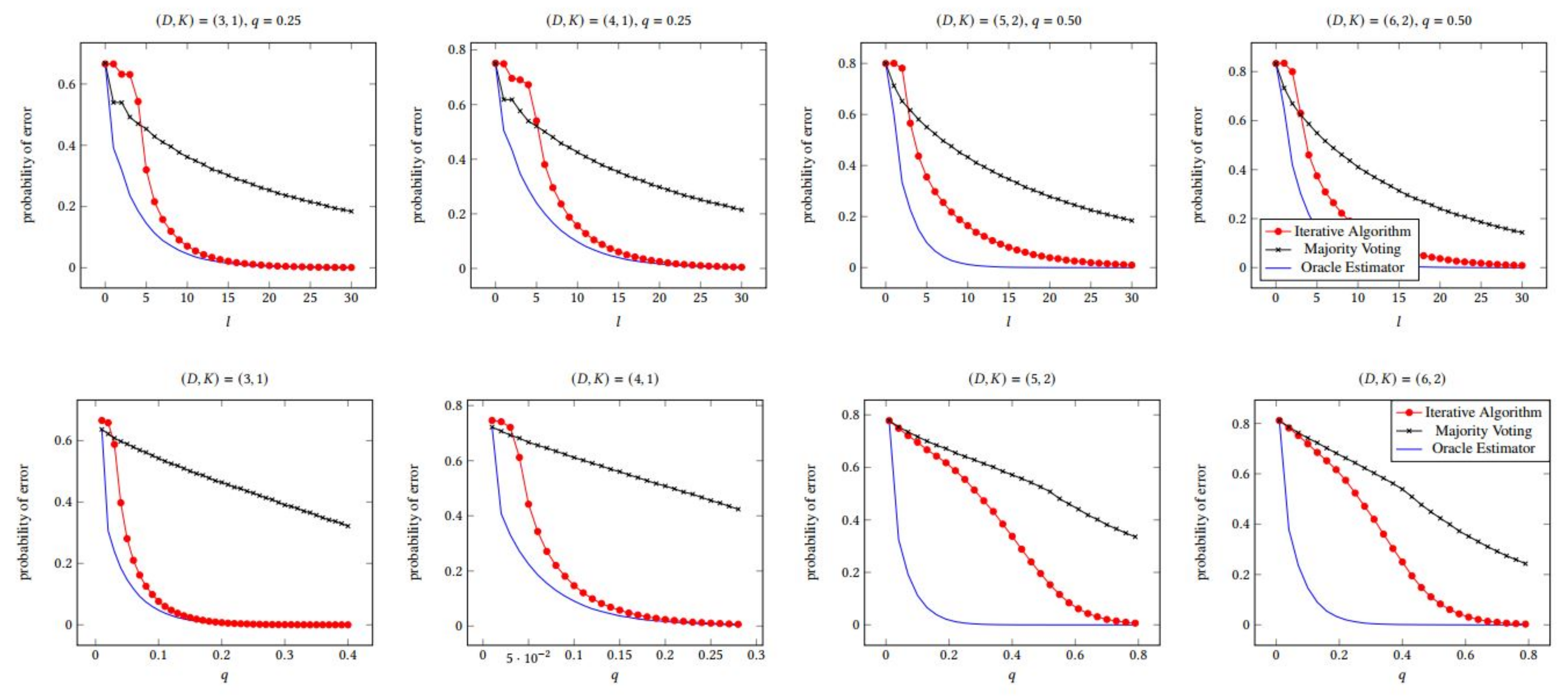
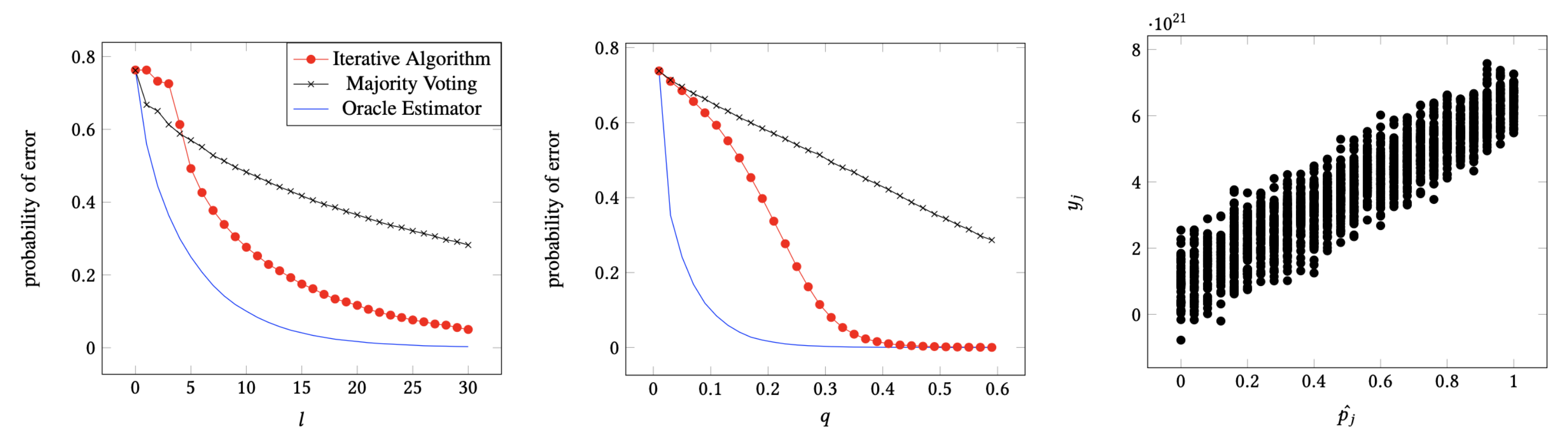
6.1. Error Performance with q and l

To show the competitiveness of our algorithm, we ran our K-approval iterative algorithm, majority voting, and the oracle estimator for 2000 tasks and 2000 workers with a fixed $(D,K)$ pair (Figure 6). Here, the oracle estimator can give each worker an appropriate weight since we assume the oracle estimator knows the quality of each worker. The error performance of the oracle estimator is presented as a lower bound. In Figure 6 (top), we can see that the probability of error decays exponentially as l increases, and is lower than that of the majority voting above the phase transition point $T=1$. In addition, Figure 6 (bottom) presents the probabilities of error decays as q increases.

As detailed in Section 5, we expect a phase transition at $T=\frac{32}{25}{\left(\frac{D-1}{D-K}\right)}^2{q}^2\widehat{l}\widehat{r}=1$ or $l=\frac{4\sqrt{2}}{5}\frac{(D-K)}{(D-1)}·\frac{1}{q}$. If we follow the result, we can expect transitions to happen around $l=4.52$ for $(3,1)$ and $(4,1)$, $l=3.39$ for $(5,2)$ and $l=3.62$ for $(6,2)$. From the experiments in Figure 6 (top), we find that the iterative algorithm starts to perform better than majority voting around $l=5,6,3,4$ for each $(D,K)$ pair. Note that these values are very similar to the above theoretical values. It follows from the fact that the error of our method increases with k when $T<1$ as stated in Section 5. As can clearly be seen from the simulation results, we can be sure that the l values required for achieving $T>1$ are not large.

6.2. Relationship between Reliability and y-Message

The inference of workers’ relative reliability in the course of iterations is the most important aspect of our algorithm. Now, we define the estimated reliability $\widehat{p_j}$ for each worker j as follows:

$$\widehat{p_j}=\frac{\#ofresponsesincludingcorrectanswer}{r_j}.$$

After $k_{max}$ iterations, we can find reliable workers by the value of the worker message $y_j$ since this value is proportional to $\widehat{p_j}$, which is influenced by $p_j$. The relative reliability $y_j$ is calculated by the following equation in Algorithm 1:

$$y_j\leftarrow \sum _{i\in \partial j}\frac{1}{K_i}\left({\overrightarrow{A}}^{ij}-\left(\frac{K_i}{D_i}\right)\overrightarrow{1}\right)·{\overrightarrow{x}}_{i\to j}^{(k_{max}-1)}$$

Figure 7 shows that there are strong correlations between $y_j$ and $\widehat{p_j}$. In one simulation, the correlation coefficients (Pearson product-moment correlation coefficient (PPMCC) was used for evaluation) between $y_j$ and $\widehat{p_j}$ were measured as 0.991, 0.992, 0.904, and 0.954 for $(D,K)=(3,1),(4,1),(5,2)$ and $(6,2)$, respectively. We can also check that the line approximately passes the point of $(\frac{K}{D},0)$, where $p_j=\frac{K}{D}$ is close to the reliability of a non-informative worker who gives random responses, as expected in Section 5.

6.3. Error Performance with Various (D,K) Pairs

To show the performance of the K-approval iterative algorithm, we performed simulations on a task set consisting of various $(D,K)$ pairs with Algorithm 1. In detail, we repeated the same experiments with a question set composed of an equal ratio of different task types whose $(D,K)$ values are $(3,1)$, $(4,1)$, $(5,2)$ and $(6,2)$. Then, we investigated for the general case that $q_j$ is calculated with a general version of Equation (4) in Section 5.1, as follows:

$$q_j\left(p_j\right)=Q\left(p_j\right)-Q\left(\frac{K_i}{D_i}\right),$$

(14)

where $Q\left(p\right)=plog\left[\frac{p}{{}_{D_i-1}{C}_{K_i-1}}\right]+(1-p)log\left[\frac{1-p}{{}_{D_i-1}{C}_{K_i}}\right]$.

We define $q_j$ as an individual inherent quality of the worker j. To perform simulations and to analyze the results, we have to make an assumption that a worker with an individual quality $q_j$ solves questions with a reliability $p_{ij}$ for each ($D_i,K_i$). Thus for each $(D_i,K_i)$-task, the corresponding reliability $p_{ij}$ is determined by applying Newton’s method on a graph of the quality function.

It can be seen that the same tendencies found in previous simulations also appear in Figure 8. There also is a strong correlation between $y_j$ and $\widehat{p_j}$, i.e., 0.929. This result is notable in that in the real world, there are many more cases where questions have various $(D,K)$ pairs rather than fixed ones.

7. Conclusions

Web-based crowdsourcing systems have evolved to encourage workers to make multiple choices among given options. These changes are primarily aimed at reducing workers’ mistakes and collecting higher-quality data. In this article, we have proposed an iterative algorithm for top-K selection questions. Moreover, our scheme covers the case with a task set consisting of various $(D,K)$ pairs (mixed). Furthermore, we proved that the performance of our algorithm is upper-bounded and the bound on the probability of error decays exponentially in terms of the quality of workers and the number of queries. We hope that our work on K-approval crowdsourcing systems will be of practical help to researchers who need to collect high-quality real data.

Presently, the proposed algorithm in this paper adopts an iterative regime; however, in future work we will generalize our algorithm with generalized task–worker allocation using evolutionary algorithms (generic algorithms and harmony search). For example, by ensuring that appropriate tasks are assigned according to each worker’s experiences, preference, and ability, a task master can increase worker efficiency and reduce the error rate.

References

1. Kittur, A.; Chi, E.H.; Suh, B. Crowdsourcing user studies with Mechanical Turk. In Proceedings of the SIGCHI Conference on Human Factors in Computing Systems, Florence, Italy, 5–10 April 2008; pp. 453–456. [Google Scholar]
2. Lintott, C.J.; Schawinski, K.; Slosar, A.; Land, K.; Bamford, S.; Thomas, D.; Raddick, M.J.; Nichol, R.C.; Szalay, A.; Andreescu, D.; et al. Galaxy Zoo: Morphologies derived from visual inspection of galaxies from the Sloan Digital Sky Survey. Mon. Not. R. Astron. Soc. 2008, 389, 1179–1189. [Google Scholar] [CrossRef] [Green Version]
3. Simonyan, K.; Zisserman, A. Very deep convolutional networks for large-scale image recognition. arXiv 2014, arXiv:1409.1556. [Google Scholar]
4. Deng, J.; Dong, W.; Socher, R.; Li, L.J.; Li, K.; Fei-Fei, L. Imagenet: A large-scale hierarchical image database. In Proceedings of the 2009 IEEE Conference on Computer Vision and Pattern Recognition, Miami, FL, USA, 20–25 June 2009; pp. 248–255. [Google Scholar]
5. Sheng, V.S.; Provost, F.; Ipeirotis, P.G. Get another label? improving data quality and data mining using multiple, noisy labelers. In Proceedings of the 14th ACM SIGKDD International Conference on Knowledge Discovery and Data Mining, Las Vegas, NV, USA, 24–27 August 2008; pp. 614–622. [Google Scholar]
6. Snow, R.; O’Connor, B.; Jurafsky, D.; Ng, A.Y. Cheap and fast—But is it good?: Evaluating non-expert annotations for natural language tasks. In Proceedings of the Conference on Empirical Methods in Natural Language Processing, Association for Computational Linguistics, Honolulu, HI, USA, 8–11 October 2008; pp. 254–263. [Google Scholar]
7. Ipeirotis, P.G.; Provost, F.; Wang, J. Quality management on amazon mechanical turk. In Proceedings of the ACM SIGKDD workshop on human computation, Washington, DC, USA, 24–28 July 2010; pp. 64–67. [Google Scholar]
8. Kazai, G.; Kamps, J.; Milic-Frayling, N. An analysis of human factors and label accuracy in crowdsourcing relevance judgments. Inf. Retr. 2013, 16, 138–178. [Google Scholar] [CrossRef]
9. Raykar, V.C.; Yu, S.; Zhao, L.H.; Valadez, G.H.; Florin, C.; Bogoni, L.; Moy, L. Learning from crowds. J. Mach. Learn. Res. 2010, 11, 1297–1322. [Google Scholar]
10. Dawid, A.P.; Skene, A.M. Maximum likelihood estimation of observer error-rates using the EM algorithm. Appl. Stat. 1979, 28, 20–28. [Google Scholar] [CrossRef]
11. Whitehill, J.; Wu, T.F.; Bergsma, J.; Movellan, J.R.; Ruvolo, P.L. Whose vote should count more: Optimal integration of labels from labelers of unknown expertise. Adv. Neural Inf. Process. Syst. 2009, 22, 2035–2043. [Google Scholar]
12. Welinder, P.; Branson, S.; Perona, P.; Belongie, S.J. The multidimensional wisdom of crowds. Adv. Neural Inf. Process. Syst. 2010, 23, 2424–2432. [Google Scholar]
13. Zhang, Y.; Chen, X.; Zhou, D.; Jordan, M.I. Spectral methods meet EM: A provably optimal algorithm for crowdsourcing. Adv. Neural Inf. Process. Syst. 2014, 27, 1260–1268. [Google Scholar]
14. Karger, D.R.; Oh, S.; Shah, D. Iterative learning for reliable crowdsourcing systems. Adv. Neural Inf. Process. Syst. 2011, 24, 1953–1961. [Google Scholar]
15. Karger, D.R.; Oh, S.; Shah, D. Budget-optimal crowdsourcing using low-rank matrix approximations. In Proceedings of the 2011 49th Annual Allerton Conference on Communication, Control, and Computing (Allerton), Monticello, IL, USA, 28–30 September 2011; pp. 284–291. [Google Scholar]
16. Liu, Q.; Peng, J.; Ihler, A. Variational inference for crowdsourcing. Adv. Neural Inf. Process. Syst. 2012, 25, 692–700. [Google Scholar]
17. Dalvi, N.; Dasgupta, A.; Kumar, R.; Rastogi, V. Aggregating crowdsourced binary ratings. In Proceedings of the 22nd international conference on World Wide Web, Rio de Janeiro, Brazil, 13–17 May 2013; pp. 285–294. [Google Scholar]
18. Lee, D.; Kim, J.; Lee, H.; Jung, K. Reliable Multiple-choice Iterative Algorithm for Crowdsourcing Systems. ACM Sigmetr. Perform. Eval. Rev. 2015, 4, 205–216. [Google Scholar] [CrossRef]
19. Ma, Y.; Olshevsky, A.; Saligrama, V.; Szepesvari, C. Crowdsourcing with Sparsely Interacting Workers. arXiv 2017, arXiv:1706.06660. [Google Scholar]
20. Su, H.; Deng, J.; Li, F.-F. Crowdsourcing annotations for visual object detection. In Proceedings of the Workshops at the Twenty-Sixth AAAI Conference on Artificial Intelligence, Toronto, ON, Canada, 22–26 July 2012; Volume 1. [Google Scholar]
21. Shah, N.B.; Zhou, D.; Peres, Y. Approval Voting and Incentives in Crowdsourcing. arXiv 2015, arXiv:1502.05696. [Google Scholar]
22. Procaccia, A.D.; Shah, N. Is Approval Voting Optimal Given Approval Votes? Adv. Neural Inf. Process. Syst. 2015, 28, 1792–1800. [Google Scholar]
23. Salek, M.; Bachrach, Y. Hotspotting-a probabilistic graphical model for image object localization through crowdsourcing. In Proceedings of the Twenty-Seventh AAAI Conference on Artificial Intelligence, Bellevue, WA, USA, 14–18 July 2013. [Google Scholar]
24. Zhou, D.; Liu, Q.; Platt, J.C.; Meek, C. Aggregating Ordinal Labels from Crowds by Minimax Conditional Entropy. In Proceedings of the International Conference on Machine Learning, Beijing, China, 21–26 June 2014; Volume 14, pp. 262–270. [Google Scholar]
25. Karger, D.R.; Oh, S.; Shah, D. Efficient crowdsourcing for multi-class labeling. In Proceedings of the ACM SIGMETRICS/International Conference on Measurement and Modeling of Computer Systems, Pittsburgh, PA, USA, 17–21 June 2013; pp. 81–92. [Google Scholar]
26. Kim, J.; Lee, D.; Jung, K. Reliable Aggregation Method for Vector Regression Tasks in Crowdsourcing. In Lecture Notes in Computer Science, Proceedings of the Pacific-Asia Conference on Knowledge Discovery and Data Mining, Singapore, 11–14 May 2020; Springer: Cham, Switzerland, 2020; pp. 261–273. [Google Scholar]
27. Kamar, E.; Hacker, S.; Horvitz, E. Combining human and machine intelligence in large-scale crowdsourcing. In Proceedings of the 11th International Conference on Autonomous Agents and Multiagent Systems-Volume 1, International Foundation for Autonomous Agents and Multiagent Systems, Spain, Valencia, 4–8 June 2012; pp. 467–474. [Google Scholar]
28. Branson, S.; Van Horn, G.; Perona, P. Lean Crowdsourcing: Combining Humans and Machines in an Online System. In Proceedings of the IEEE Conference on Computer Vision and Pattern Recognition (CVPR), Honolulu, HI, USA, 21–26 July 2017. [Google Scholar]
29. Van Horn, G.; Branson, S.; Loarie, S.; Belongie, S.; Perona, P. Lean multiclass crowdsourcing. In Proceedings of the IEEE Conference on Computer Vision and Pattern Recognition, Salt Lake City, UT, USA, 18–22 June 2018; pp. 2714–2723. [Google Scholar]
30. Yin, X.; Wang, H.; Wang, W.; Zhu, K. Task recommendation in crowdsourcing systems: A bibliometric analysis. Technol. Soc. 2020, 63, 101337. [Google Scholar] [CrossRef]
31. Zhou, C.; Tham, C.K.; Motani, M. Online auction for scheduling concurrent delay tolerant tasks in crowdsourcing systems. Comput. Netw. 2020, 169, 107045. [Google Scholar] [CrossRef]
32. Dashtipour, K.; Gogate, M.; Li, J.; Jiang, F.; Kong, B.; Hussain, A. A hybrid Persian sentiment analysis framework: Integrating dependency grammar based rules and deep neural networks. Neurocomputing 2020, 380, 1–10. [Google Scholar] [CrossRef] [Green Version]
33. Basiri, M.E.; Kabiri, A. Words are important: Improving sentiment analysis in the Persian language by lexicon refining. ACM Trans. Asian Low-Resour. Lang. Inf. Process. (TALLIP) 2018, 17, 1–18. [Google Scholar] [CrossRef]
34. Ye, B.; Wang, Y.; Liu, L. Crowd trust: A context-aware trust model for worker selection in crowdsourcing environments. In Proceedings of the 2015 IEEE International Conference on Web Services, New York, NY, USA, 27 June–2 July 2015; pp. 121–128. [Google Scholar]
35. Cui, Q.; Wang, S.; Wang, J.; Hu, Y.; Wang, Q.; Li, M. Multi-Objective Crowd Worker Selection in Crowdsourced Testing. In Proceedings of the SEKE, Pittsburgh, PA, USA, 5–7 July 2017; Volume 17, pp. 1–6. [Google Scholar]
36. Vargas-Santiago, M.; Monroy, R.; Ramirez-Marquez, J.E.; Zhang, C.; Leon-Velasco, D.A.; Zhu, H. Complementing Solutions to Optimization Problems via Crowdsourcing on Video Game Plays. Appl. Sci. 2020, 10, 8410. [Google Scholar] [CrossRef]
37. Moayedikia, A.; Yeoh, W.; Ong, K.L.; Boo, Y.L. Improving accuracy and lowering cost in crowdsourcing through an unsupervised expertise estimation approach. Decis. Support Syst. 2019, 122, 113065. [Google Scholar] [CrossRef]
38. Karger, D.R.; Oh, S.; Shah, D. Budget-Optimal Task Allocation for Reliable Crowdsourcing Systems. Oper. Res. 2014, 62, 1–24. [Google Scholar] [CrossRef] [Green Version]
39. Alon, N.; Spencer, J.H. The Probabilistic Method; John Wiley & Sons: Hoboken, NJ, USA, 2008. [Google Scholar]
Figure 1. A task in the Amazon Mechanical Turk, whose goal is to categorize the item in the picture. The worker is allowed to choose two candidates.
Applsci 11 00630 g001
Figure 2. A task being distributed on Zooniverse to correctly figure out what animals Wisconsin wildlife are pictured. The worker is allowed to choose multiple candidates.
Applsci 11 00630 g002
Figure 3. An illustration of task–worker assignments.
Applsci 11 00630 g003
Figure 4. Description of a task message x i j ( k ) and a response vector A i j in the message vector space when A i j = ( 1 , 1 , 0 ) and D = 3 , K = 2 .
Applsci 11 00630 g004
Figure 5. Comparison of quality between negative entropy with offset and 4th-order polynomial approximation.
Applsci 11 00630 g005
Figure 6. Comparisons of probabilities of error between different algorithms varying l (first row) and q (second row) values ( m = n = 2000 , l = r = 25 ).
Applsci 11 00630 g006
Figure 7. Relationship between true y j and the estimated p j ^ after ten iterations ( m = n = 2000 , k = 10 ).
Applsci 11 00630 g007
Figure 8. Simulations on a set of various ( D , K ) pairs ( m = n = 2000 , mixed task types: ( D , K ) = ( 3 , 1 ) , ( 4 , 1 ) , ( 5 , 2 ) , ( 6 , 2 ) ) at an equal ratio.
Applsci 11 00630 g008
Publisher’s Note: MDPI stays neutral with regard to jurisdictional claims in published maps and institutional affiliations.