Featured Application
This work is used for calibrating intrinsic parameters of camera and extrinsic parameters between camera and flash LiDAR.
Abstract
Calibration between multiple sensors is a fundamental procedure for data fusion. To address the problems of large errors and tedious operation, we present a novel method to conduct the calibration between light detection and ranging (LiDAR) and camera. We invent a calibration target, which is an arbitrary triangular pyramid with three chessboard patterns on its three planes. The target contains both 3D information and 2D information, which can be utilized to obtain intrinsic parameters of the camera and extrinsic parameters of the system. In the proposed method, the world coordinate system is established through the triangular pyramid. We extract the equations of triangular pyramid planes to find the relative transformation between two sensors. One capture of camera and LiDAR is sufficient for calibration, and errors are reduced by minimizing the distance between points and planes. Furthermore, the accuracy can be increased by more captures. We carried out experiments on simulated data with varying degrees of noise and numbers of frames. Finally, the calibration results were verified by real data through incremental validation and analyzing the root mean square error (RMSE), demonstrating that our calibration method is robust and provides state-of-the-art performance.
1. Introduction
Recently, a considerable amount of literature has proliferated around the theme of multi-sensor systems in 3D object detection and recognition [1], simultaneous localization and mapping (SLAM) [2], path planning [3], reconstruction scenes [4,5], and other fields. In these fields, visual and depth information are the most widely used elements to recognize the environment. A camera can acquire color information of the target with such advantages as small size, low cost, and high resolution. However, it is difficult to acquire the distance between the target and camera. Three-dimensional light detection and ranging (LiDAR) can obtain accurate depth data of the target. In brief, by fusing a camera and LiDAR sensors, we can utilize their advantages and complement their disadvantages to perceive the environment comprehensively. To achieve this purpose, we need to get the relative positions and orientations between the camera and LiDAR by calibrating the system.
LiDAR systems can be classified into two categories, mechanical scanning LiDAR and solid-state LiDAR. The former typically comprises one or more laser and detector pairs, which are mounted on a rotating or vibrating scanner [6]. Mechanical scanning LiDAR is first developed and used in many applications: urban planning, urban mapping, intelligent autonomous transport, and scanning forests and agricultural fields [7,8,9]. It is a mature technology, however, the use of a mechanical scanner increases the system size and complexity, while challenging the reliability of the moving parts under long-term use. A solid-state LiDAR is usually a radar with no moving parts at all. It mainly includes micro electro mechanical systems (MEMS) LiDAR, optical phased array (OPA) LiDAR, and flash LiDAR. MEMS LiDAR do not completely cancel the mechanical moving structure [10]. The mechanical structure is integrated into a small silicon-based chip by MEMS technology, inside which there is a rotatable MEMS micro-mirror, through which the transmitting angle of a single transmitter is changed. OPA LiDAR consists of an array of light-emitting elements where the phase can be manipulated [11]. On top of that, the entire system is fabricated on a single chip using a silicon photonics platform. Flash LiDAR illuminates the entire scene in a single shot and detects the light reflected from the scene with an array of detectors [12]. As there are no moving parts, solid-state LiDAR systems can be built with enhanced reliability.
Camera and LiDAR system calibration consists of intrinsic calibration and extrinsic calibration. The intrinsic parameters of the camera are related to the characteristics of the camera itself, including focal length and size of pixels. In most literature, it is accepted that the intrinsic parameters of the camera are calibrated in advance. The intrinsic parameters of LiDAR sensors are calibrated in the factory. The extrinsic calibration is to find the rotation and translation relationship between the camera and LiDAR.
In this paper, we present a novel method to calibrate the intrinsic parameters of the camera and extrinsic parameters of the system. Our work has four characteristics differentiating itself from prior research:
- The traditional calibration method has limited accuracy because of low vertical resolution of 3D mechanical scanning LiDAR. For instance, Velodyne-64 LiDAR can only measure 64 channels vertically, and generate sparse point clouds of the environment. Our method deals with dense point cloud, thus the result has high accuracy. We first apply flash LiDAR to acquire dense point clouds both in the horizontal direction and vertical direction to improve calibration accuracy.
- We design a novel calibration target made up of an arbitrary triangular pyramid, with three chessboards on it. The sizes of the triangular pyramid are unknown, and it can be unsymmetrical, hence the manufacturing of the pyramid has no effect on the accuracy. Our method only employs planes of triangular pyramid from camera images and LiDAR point clouds in calibration.
- Unlike most methods, our method can obtain intrinsic parameters of the camera and extrinsic parameters of the system together. It only takes one capture of the camera and LiDAR to get the intrinsic parameters and extrinsic parameters of the system. Moreover, we employ an optimization algorithm to reduce errors by minimizing the distance between the 3D points and target plane.
- More frames of the camera and LiDAR can improve accuracy by aligning the triangular pyramid planes of all frames. We also use simulation and incremental experiment to verify the precision and stability.
To explain and explore the proposed calibration method, we organize the remainder of this paper as follows. In Section 2, we investigate previous work with regard to calibration between the camera and LiDAR briefly. In Section 3, the calibration target and the proposed method are described in detail. The experiments and results analysis on both simulation and real test are exhibited in Section 4. Finally, conclusions and future work are provided in Section 5.
2. Related Works
The calibration of the camera and LiDAR system contains intrinsic parameters and extrinsic parameters. The intrinsic calibration method of the camera varies with calibration objects. Traditional camera intrinsic calibration techniques such as Zhang’s algorithm [13] make use of a calibration board with a checkerboard pattern on it. The methods of [14] and [15] both focus on obtaining the coordinate of the feature points to solve the intrinsic parameters. The former designs a novel 3D calibration board with local gradient depth information and main plane square corner information(BWDC), while the latter uses a polygonal planar board. Most research on calibration between the camera and LiDAR ignored the camera calibration. The intrinsic parameters of LiDAR are completed by manufacturers. The method of [16] describes a way to obtain intrinsic parameters of 3D mechanical scanning LiDAR. The authors of [17] report on a calibration and stability analysis of the Velodyne VLP-16 LiDAR scanner. In this paper, we apply flash LiDAR calibrated in advance, and the method to obtain the intrinsic parameters of the camera is described amply in Section 3.2.1.
Similar to camera intrinsic calibration, the extrinsic calibration method between the camera and LiDAR is closely related to the calibration object. There are currently two basic categories in calibration research. One is target calibration, and the other is targetless calibration. Early target calibration methods focus on camera and 1D or 2D LiDAR system. With the development of 3D LiDAR techniques, study concentration moved to the combination of camera and 3D mechanical scanning LiDAR. The indispensable geometric constraints can also be divided into two categories: vector constraint and feature point. The works of [18,19,20,21,22] utilize normal vectors of plane boards to find the expression in both image and point clouds, and then calculate the conversion between camera and LiDAR. A further paper [18] first adopts this idea to calibrate a 2D range finder and camera system. Another paper [19] further makes a toolbox online by extending this method to 3D LiDAR and camera system. The work of [20] uses three checkerboards and minimizes an energy function of correspondences between depth and image frames. Other works [21,22] take several captures of calibration target and align normal vectors of these planes to iteratively obtain the calibration result. The work of [23] introduces the 3D line correspondence into the original plane correspondence and reduces the minimal number of poses required for this problem to one.
The works of [14,15,24,25,26] apply the feature point correspondences calibration method. Two-dimensional feature points in images can be conveniently acquired, whereas obtaining the corresponding 3D feature points in point clouds is challenging as the point clouds of LiDAR are sparse. The authors of [14] apply 3D-2D point correspondences to calibrate the product of intrinsic matrix and extrinsic matrix, while [15] combines 3D-2D and 3D-2D point correspondences together. In recent years, a small number of studies focus on using the structural similarity between the LiDAR point cloud and image data to perform global matching and optimize the calibration results [27,28,29]. The method of [27] incorporates the laser reflectivity of 3D LiDAR points for calibration. Another paper [28] calibrates by maximizing the mutual information between the intensity of the LiDAR frame and the gray information of the image. A further paper [29] adopts the natural alignment of depth and intensity edges in combination with a Gaussian mixture model to accomplish the calibration. However, the targetless method need a large number of data and the sparse point clouds decrease the accuracy of the matching results.
To improve the calibration accuracy and simplify manual operation, we apply flash LiDAR and propose a novel method to calibrate the intrinsic parameters of the camera and extrinsic parameters of the system. In addition, the proposed method can also be applied to calibrate multiple cameras and multiple LiDAR systems if they can capture the target simultaneously.
3. Method
3.1. Problem Formulation
The calibration of the camera and LiDAR system basically contains four coordinate systems. In this paper, the definition goes as follows. The camera coordinate system is represented as (the origin is the optical center of camera). The LiDAR coordinate system is noted as (the origin is the intersection point of the laser beams). The pixel coordinate system is defined as (the origin is the first pixel of camera or LiDAR), as shown in Figure 1. The world coordinate system is denoted as (described in detail in Section 3.2). Moreover, we use italic lowercase, italic uppercase, and boldfaced uppercase letters to represent scalars, vectors, and matrices, respectively, throughout this paper.
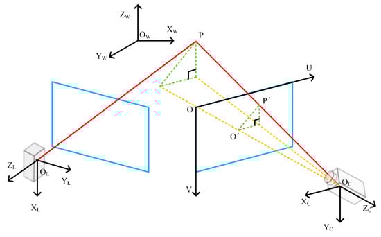
Figure 1.
Intrinsic parameters calibration model of camera and flash light detection and ranging (LiDAR). Arbitrary point P of object is projected onto flash LiDAR (left) and camera (right).
3.1.1. Intrinsic Parameters Calibration Problem Formulation
As mentioned above, we apply flash LiDAR to complete calibration of the system because of its low cost and high resolution in both the vertical and horizontal directions. Besides, flash LiDAR has a big advantage in terms of price and stability. The LiDAR emits a beam of diverging laser initiatively, and the light returns to LiDAR through optical lens on a light-sensitive chip. This process follows time of flight (TOF) theory and calculates how long it takes for the light to hit an object and reflect back to the LiDAR. Hence, the intrinsic parameters of the camera and flash LiDAR both can be demonstrated by the pinhole model, as illustrated in Figure 1. The mere difference is that the pixel value of camera refers to color information, while the pixel value of LiDAR represents distance. The basic assumption here is that the lens distortion is dismissed.
Arbitrary point on the object is captured by camera or LiDAR. The projection of is point on the image plane. According to triangle similarity, we can obtain the coordinate relationship of projection:
where denotes the coordinate of point in the camera coordinate system (or LiDAR coordinate system), and is noted as the projection of point in pixel coordinate system. represents the coordinate of the center point on the image. and refer to the camera sensor pixel size. represents the effective focal length.
We can obtain the relationship of coordinate between the camera coordinate system (or LiDAR coordinate system) and pixel coordinate system by combining Equation (1):
where , . The intrinsic parameters of the camera and flash LiDAR are , , , and , and matrix is defined as the intrinsic matrix.
Our method improves on the method of [13], in terms of the acquisition of intrinsic parameter of the camera described in Section 3.2.1, and the intrinsic parameters of flash LiDAR are calibrated in advance by the manufacturer.
3.1.2. Extrinsic Parameters Calibration Problem Formulation
The extrinsic calibration problem is demonstrated in Figure 2a. During once calibration, the camera and LiDAR are fixed firmly. The calibration target is in a suitable position, where it can be captured by the camera and LiDAR simultaneously. The core of the extrinsic calibration problem is to estimate the relative pose between the camera coordinate system and LiDAR coordinate system. Assuming that the coordinates of arbitrary point in the camera coordinate system and LiDAR coordinate system are and , the transformation of them can be shown as follows:
where rotation matrix and translation vector are extrinsic parameters of the camera and LiDAR system. The details of our extrinsic calibration method are shown in Section 3.2.2.
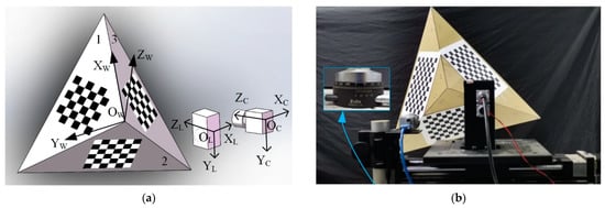
Figure 2.
Sketch map of calibration target and camera-flash system: (a) extrinsic parameters calibration model; (b) camera is fixed on a precise rotation stage, and flash LiDAR is fixed on a precise motorized linear stage.
3.2. Methodology
We design a triangular pyramid calibration target to complete the calibration of the camera and flash LiDAR system. The target is an arbitrary triangular pyramid with a chessboard pasted on its three planes, as shown in Figure 2a. Without knowing the size of the triangular pyramid, the only parameter to be determined is the size of the unit of the chessboard, hence the error of manufacture being ignored. In this section, the world coordinate system is set up as follows. Origin is the middle vertex of the triangular pyramid. Axis is aligned with one edge of the triangular pyramid. Axis is on plane 1, perpendicular to axis . The direction of axis is determined by the right hand rule.
3.2.1. Intrinsic Parameters Calibration of Camera
Zhang’s method [13] finds the corner points correspondence of the chessboard to estimate the intrinsic parameters of the camera. However, it needs too many captures to get a good result. Our method makes some improvements by calibration with only one capture. As shown in Figure 2a, the camera can acquire the image of three chessboards during a single shot. Then, we need to separate the image into three districts roughly by hand, which is rather easy to do. Assuming that the equation of each chessboard plane is , the corner point of each chessboard can be expressed as . According to the coordinates’ transformation and intrinsic parameter model in Section 3.1.1, the conversion between the chessboard coordinate and pixel coordinate can be established as follows:
where and represent the coordinate of corner points in the camera coordinate system and chessboard coordinate system. We define the following:
where is the homography matrix, figured out by four pairs of feature points according to Equation (4). The rotation vector and are orthogonal to each other and as normal vectors, they satisfy the following:
Hence, one chessboard can provide two equations of intrinsic matrix . The triangular pyramid target has three chessboards on its planes and can provide six equations of , sufficient to work it out. Then, three pairs of rotation vectors and can be figured out according to Equation (6), which are used in Section 3.2.2.
3.2.2. Extrinsic Parameters Calibration between Camera and Flash LiDAR
Our method applies a geometric constraint of the triangular pyramid target to calibrate the extrinsic parameters. The method estimates the rotation matrix and translation vector from to (and ) separately. Finally, we can obtain the extrinsic parameters from to .
It is essential to convert the pixel values of LiDAR to 3D point clouds. As mentioned in Section 3.1.1, the output of flash LiDAR is the distance between the object and LiDAR on each pixel. The relation between the coordinate of the arbitrary point in and distance is as follows:
where represents the distance between origin and point , which can be acquired by each pixel value of LiDAR. Utilizing the intrinsic parameters of flash LiDAR offered by manufacturers, we can obtain the relationship between the pixel coordinate system and LiDAR coordinate system according to Equation (1):
To calibrate the extrinsic parameter between and , we adopt a 3D plane fitting method based on the RANSAC algorithm to acquire the equation of three planes of the triangular pyramid, and the steps can be described as follows:
- Apply Kmeans cluster algorithm [30] to acquire point cloud of triangular pyramid target apart from background points.
- Select three points from point cloud P of triangular pyramid, and calculate the equation of the plane formed by these three points.
- Classify the other points to either inlier point or outlier point by comparing the distance between these points and the plane to a threshold value, and tally the amount of inlier points.
- Repeat steps (2) and (3) a certain number of times to find the first best plane, or until the amount of inlier points reaches a threshold value.
- Remove the inlier points and repeat steps (2), (3), and (4) twice to find the second and third best planes.
Then, we can obtain the equations of plane in :
where is arbitrary point of plane , vector represents the unit normal vector of plane , and denotes the distance of origin and plane . The coordinate of origin can be calculated by Equation (10), and normal vectors of three axes can be determined by cross product:
Then, we can obtain the rotation matrix and translation vector from the world coordinate system to LiDAR coordinate system:
The next step is to estimate the rotation matrix and translation vector from the world coordinate system to camera coordinate system. This time, we need to acquire the expressions of plane in . Knowing the intrinsic parameters of the camera in Section 3.2.1, we can obtain the rotation matrix and translation vector from each chessboard to the camera coordinate system by Equation (5). Then, the origin and unit normal vector of chessboard can be transformed to by the following:
where represents unit normal vector of chessboard , and denotes the origin coordinate of chessboard . The expression of plane in can be acquired:
where is an arbitrary point on plane . Similar to Equation (10), the coordinate of origin is as follows:
Normal vectors of three axes , , and can also be determined by Equation (11). Hence, the rotation matrix and translation vector from to are as follows:
Then, we can obtain rotation matrix and translation vector from to by coordinate system transformation:
where and are the initial rigid transformation of system. However, there are errors caused by LiDAR point cloud and camera image. To reduce errors, we project point cloud of the triangular pyramid to the camera coordinate system and minimize the distance between all points and corresponding chessboards.
where represents the amount of inlier points belonging to plane and denotes the th point of plane . This non-liner optimization problem can be solved by the Levenberg Marquardt algorithm [31].
3.2.3. Calibration Problem Restated
The proposed method can estimate the intrinsic parameters and extrinsic parameters through a single capture of the camera and LiDAR in Section 3.2.1 and Section 3.2.2. We can further increase the accuracy by acquiring more data. Keeping the camera and LiDAR static, we randomly move the triangular pyramid times. Each time, the camera and LiDAR frame are denoted by and , where . According to Equation (5), the intrinsic parameter calibration problem of the camera can be formulated according to the equations below:
where . Hence, we have equations of Equation (20), and it can be estimated by the Levenberg Marquardt algorithm [31]. The extrinsic calibration problem can be transformed to the optimization of the rotation matrix and translation vector separately. After rigid transformation, the unit normal vectors of and are aligned to each other.
where and represent the unit normal vectors of plane in and , available by the Singular Value Decomposition (SVD) method. After rigid transformation, the points of triangular pyramid are on the chessboard plane, formulated by the following:
where is the amount of points of plane in frame , and are the expression of plane in frame according to Equation (9), and denotes the th point of plane in frame . The translation vector can also be estimated by the Levenberg Marquardt algorithm [31].
Figure 3 is a flow chart of our method to calibrate the camera and flash LiDAR system. Firstly, we turn on the camera and LiDAR to acquire image and point cloud of the triangular pyramid target simultaneously. The image of the target is divided into three parts and each part displays the image of one chessboard. Secondly, we apply the feature points correspondence method based on [13] to obtain homography matrix and intrinsic matrix of the camera. Thirdly, we calculate rigid transformation from the chessboard to camera by combining and to obtain the extrinsic parameters from the world coordinate system to camera coordinate system. At the same time, we fit planes of three chessboards in the point cloud and obtain extrinsic parameters from the world coordinate system to LiDAR coordinate system. Finally, we calculate the initial extrinsic parameters from the LiDAR coordinate system to camera coordinate system, and optimize the result by minimizing the distance from the points to the chessboard. Furthermore, if we take more frames of the camera and LiDAR, the result can be more accurate by applying the Levenberg Marquardt algorithm [31].
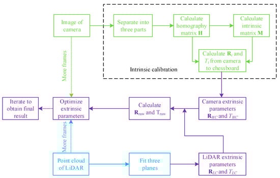
Figure 3.
Flowchart of intrinsic and extrinsic calibration of the proposed method.
4. Experiments
A series of experiments are implemented to analyze the performance of the proposed method. First, we test the algorithm by simulation and observe the sensibility of noise. Then, a real camera and flash LiDAR system is calibrated with incremental verification experiments. Finally, the method is verified on a depth map.
4.1. Simulation
4.1.1. Experiment Settings
We first evaluate our extrinsic calibration method by simulation data and ground truth. We set up a virtual camera and flash LiDAR system. The intrinsic parameters of the virtual camera and flash LiDAR are shown in Table 1. The rotation and translation from LiDAR to camera are set as and separately. The base and height of the triangular pyramid are set as 1 m and 0.4 m, respectively. The size of each cell of chessboard is 0.05 m × 0.05 m. Each plane of triangular pyramid has 6000 LiDAR points and 100 image corner points. In the following experiments, we employ and to evaluate the errors of rotation and translation:
where and are extrinsic parameters figured out through our method, and are ground truth of rotation matrix and translation vector. represents a single angle for to rotate to coincide with .

Table 1.
Parameters of virtual camera and flash light detection and ranging (LiDAR).
4.1.2. Performance with Respect to Noise on Point Cloud
The errors of depth data during LiDAR measurement and corner points during camera measurement are primary error sources in the extrinsic calibration process. In this experiment, we explore the calibration result with respect to noise on point cloud. Zero mean Gaussian noise is added to the direction vector of LiDAR point so as to simulate real measurement. The standard deviation of noise is changed from 0.01 m to 0.1 m. For each noise level, 300 independent tests are carried out. The absolute errors of rotation and translation are demonstrated in Figure 4. In the boxplot, the horizontal boundaries of the box represent the first and third quartiles, separated by the red middle line, which is the data’s median. And red points represent average absolute errors of each noise level. From Figure 4, we can observe that noise increases almost linearly with the increasing of noise level. Hence, reducing noise error of LiDAR point is an essential way to obtain an accurate calibration result. When , which is the noise level of a normal flash LiDAR, the average error of rotation is about 0.5° and the average error of translation is about 7.4 mm.
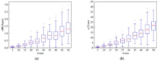
Figure 4.
The relation between absolute errors and point cloud noise level: (a) absolute errors of rotation and (b) absolute errors of translation.
4.1.3. Performance with Respect to Noise on Image Point
Pixel noise on corner points of image is another error source during measurement. In this experiment, we investigate the sensitivity of our method with reference to pixel noise. Zero mean Gaussian noise is added to the pixel of corner points on the chessboard. The standard deviation of noise varied from 0.1 pixel to 1 pixel. Similar to Section 4.1.2, 300 independent tests are carried out for each noise level. The absolute errors of rotation and translation are shown in Figure 5. From the boxplot, we can observe that the errors of rotation and translation are linear with pixel noise level. The errors caused by pixel noise are smaller than errors caused by point cloud noise. Even , the average error of rotation is about 0.16°, and the average error of translation is about 2.7 mm.
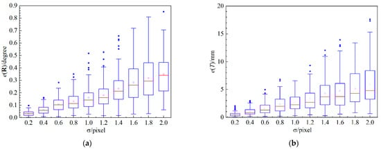
Figure 5.
The relation between absolute errors and pixel noise level: (a) absolute errors of rotation and (b) absolute errors of translation.
4.1.4. Performance with Respect to the Optimization Method
As expounded in Section 3.2.2, we utilize Equation (19) to optimize the extrinsic parameters. This experiment displays the effectiveness of our optimization method. We also carried out 300 independent trials for each noise level in Section 4.1.2 and Section 4.1.3. Figure 6 shows the relation of absolute errors and point cloud noise level after optimization.
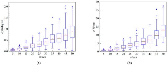
Figure 6.
The relation between absolute errors and point cloud noise level after optimization: (a) absolute errors of rotation; and (b) absolute errors of translation.
Figure 7 shows the relation of absolute errors and pixel noise level after optimization. It is clear that, after optimization, the errors of rotation and translation are both lower than initial results to some extent. In Figure 6, when , the average errors of rotation and translation are about 0.38° and 4 mm (the corresponding results in Figure 4 are 0.5° and 7.4 mm), respectively. In Figure 7, when , the average error of rotation and translation are about 0.13° and 2.2 mm (the corresponding result in Figure 5 are 0.16° and 2.7 mm), respectively. The performance means that the optimization method is effective in decreasing errors of both rotation and translation.
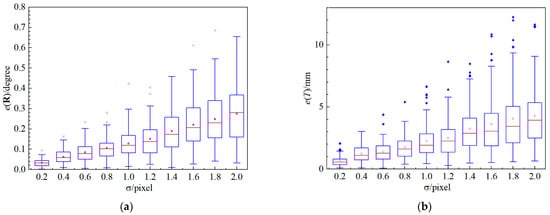
Figure 7.
The relation between absolute errors and pixel noise level after optimization: (a) absolute errors of rotation and (b) absolute errors of translation.
4.1.5. Performance with Respect to Number of Frames
As described in Section 3.2.2, our method can calibrate the extrinsic parameters through one single capture. However, more frames of the camera and LiDAR can provide more information of the target. In this experiment, we simulate 20 frames of the camera and LiDAR, and randomly select several frames to figure out the calibration result. The number of frames varied from 1 to 9, and for each number, we conduct 300 independent tests. The noise level of pixel noise is set to , and the of point cloud noise is set from 10 mm to 50 mm separately. Figure 8 and Figure 9 plot the average absolute errors of rotation and translation. It is shown that, as the number of frames increases, the rotation and translation errors decrease obviously. However, when there are more than six frames, the decrease in the measurement error is not obvious. So, it is wise to use a suitable number of frames to obtain a precise result.
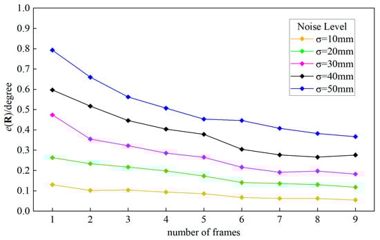
Figure 8.
Average absolute error of rotation for different number of frames.
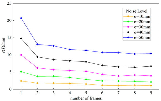
Figure 9.
Average absolute error of translation for different number of frames.
4.2. Real Data Experiments
4.2.1. Experiment Settings
The method is further evaluated by a real camera and flash LiDAR system as shown in Figure 2b. The camera is fixed on a precise rotation stage, and the flash LiDAR is fixed on a precise motorized linear stage. The parameters of flash LiDAR are provided by the manufacturers, as shown in Table 2. The horizontal resolution of flash LiDAR is 50°/320 = 0.156°, and the vertical resolution is 40°/240 = 0.167°. We can acquire 320 × 240 = 76,800 points. The resolution of camera is 1280 × 1024 and the size of cell is 20 um × 20 um. The triangular pyramid used in this experiment is about 1 m in base and about 0.4 m in height, whose size need not be known. The size of the chessboard cell is 0.05 m × 0.05 m.
Table 2.
Parameters of flash LiDAR.
4.2.2. Performance of Intrinsic Calibration
In this section, we utilize the reprojection error to verify our intrinsic parameters calibration method of the camera.
where N is the number of corner points on one chessboard, and are the theoretical coordinate and experimental coordinate of each corner point.
We take 20 images of the triangular pyramid with different positions and angles. Each image is divided to three parts by hand. Then, we calculate the intrinsic parameters of the camera and reprojection error of 20 images. Figure 10a shows the result of each image. The reprojection error of each image is below 0.5 pixel, and most are about 0.35 pixel.
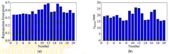
Figure 10.
Average reprojection error and root mean square error (RMSE) of 20 frames of the camera and LiDAR: (a) reprojection error and (b) RMSE.
4.2.3. Performance of Extrinsic Calibration with Number of Frames
To test the performance of a different number of camera and LiDAR frames, we keep the camera and LiDAR fixed, move the triangular pyramid randomly, and take 20 pairs of frames. One to nine pairs of frames are randomly selected to calibrate the extrinsic parameters, and we conduct 100 repeated tests for each frame level, expect that 1 frame is only tested 20 times. We also use Equation (23) to describe the single angle and translation from LiDAR to camera. The boxplot of each number of frames is shown in Figure 11.
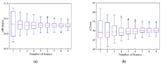
Figure 11.
Extrinsic parameters of the camera and LiDAR system: (a) rotation from LiDAR to camera and (b) translation from LiDAR to camera.
4.2.4. Performance of Root Mean Square Error
Our method employs geometric constraints of the triangular pyramid target to calibrate the extrinsic parameters of the camera and LiDAR system. There are no feature points for flash LiDAR to detect and we cannot use the reprojection error to evaluate the calibration result, as the conventional method did. Therefore, we apply root mean square error (RMSE) in this experiment.
where represents the RMSE of all points to their corresponding chessboards. We also calculate the RMSE of 20 pairs of frames, and the result is illustrated in Figure 10b. It shows that the RMSEs of most frames are under 25 mm.
4.2.5. Incremental Verification Experiments
The difficulty of evaluating extrinsic calibration lies in the difficulty to obtain the ground truth of rotation and translation between the camera and LiDAR. For this reason, we employ incremental verification experiments to evaluate the proposed method. As shown in Figure 2b, the camera is fixed on precise rotation stage and LiDAR is fixed on precise motorized linear stage. First, we calibrate extrinsic parameters of system using five pairs of frames through our method. Then, we move the precise motorized linear stage 80 mm away from camera, and we calibrate extrinsic parameters of system again. The translation vector between the first time and second time is shown in Table 3. Similarly, we rotate the precise rotation stage 11° clockwise, and figure out the rotation matrix before and after the rotating stage as well. The result is shown in Table 3.
Table 3.
Translation and rotation incremental verification results.
The increment of translation is 79.383 mm, and the error is within 0.8%. The increment of rotation is 11.041°, and the error is within 0.4%. This indicates that the error of extrinsic parameters is within the tolerance range and the results of our method are basically accurate.
4.3. Comparisons of Different Calibration Methods
In this section, we use the reprojection error to compare different calibration methods. The work of [15] applies two chessboards and one auxiliary calibration object to calibrate the extrinsic parameters of the camera and LiDAR system. They combine ten pairs of 3D-2D and 3D-3D point correspondences. The work of [32] employs more than three diamond planar boards and extracts four vertexes of each board to obtain the intrinsic and extrinsic parameters. The work of [28] is a targetless method and maximizes the mutual information between the sensor-measured surface intensities to calibrate the extrinsic parameters. The work of [33] proposes a method based on supervised learning to calibrate the extrinsic parameters.
As shown in Table 4, the reprojection error of our method is 0.390, much smaller than other methods. Moreover, our proposed method can calibrate both the intrinsic parameters of camera and extrinsic parameters of the camera and LiDAR system.
Table 4.
Comparison of different calibration methods.
4.4. Verification on Composition of Data
In order to test the actual effect of the proposed method, we use our calibration result to reconstruct 3D scenes. The 2D image of camera is superimposed to 3D point cloud of flash LiDAR, and the result is shown in Figure 12. As one can see in Figure 12c, the image of the camera and point cloud of LiDAR match quite well.
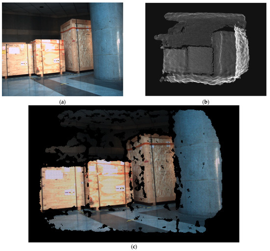
Figure 12.
Composition of 2D image and 3D point cloud: (a) 2D image captured by camera; (b) 3D point cloud captured by flash LiDAR; and (c) result of superimposing 2D image to 3D point cloud using calibration parameters through the proposed method.
5. Conclusions
Up to now, far too little attention has been paid to the fusion of the camera and flash LiDAR system. In this paper, we present a novel method of calibrating the camera and flash LiDAR system, as the traditional calibration method has limited accuracy, restricted by mechanical scanning LiDAR. Making use of dense point cloud from flash LiDAR, the proposed method has state-of-the-art accuracy. We design a calibration target that is an arbitrary triangular pyramid with three chessboards on its planes. With abundant 2D information of the chessboards, we can obtain the intrinsic parameters of the camera, and then utilize three planes of the triangular pyramid to obtain the extrinsic parameters of the system. The extrinsic parameters can be optimized by minimizing the distance between points in the LiDAR coordinate system and chessboards in the camera coordinate system. Through the proposed method, one pair capture of the camera and LiDAR is enough to calibrate the intrinsic parameters of the camera and extrinsic parameters of the system. More pairs of frames can increase the accuracy. Emulation experiments demonstrate that our method is robust to sensor noise. Moreover, we use RMSE to evaluate the accuracy and the calibration result is shown by incremental verification experiments. In the future, we will make efforts to increase the resolution of flash LiDAR to obtain a more accurate result.
Author Contributions
Conceptualization, Z.B.; methodology, Z.B.; software, Z.B.; validation, Z.B.; formal analysis, H.D.; writing—original draft preparation, Z.B.; writing—review and editing, C.S. and P.W. All authors have read and agreed to the published version of the manuscript.
Funding
This research was funded by Science and Technology on Electro-optic Control Laboratory (201951048002).
Institutional Review Board Statement
Not applicable.
Informed Consent Statement
Not applicable.
Data Availability Statement
The raw/processed data required to reproduce these findings cannot be shared at this time as the data also forms part of an ongoing study.
Conflicts of Interest
The authors declare no conflict of interest.
References
- Cho, H.; Seo, Y.W.; Kumar, B.V.K.V.; Rajkumar, R. A Multi-sensor Fusion System for Moving Object detection and Tracking in Urban Driving Environments. In Proceedings of the IEEE International Conference on Robotics and Automation (ICRA), Hong Kong, China, 31 May–7 June 2014; pp. 1836–1843. [Google Scholar]
- Yu, N.; Wang, S. Enhanced Autonomous Exploration and Mapping of an Unknown Environment with the Fusion of Dual RGB-D Sensors. Engineering 2019, 5, 164–172. [Google Scholar]
- Wan, S.; Zhang, X.; Xu, M.; Wang, W.; Jiang, X. Region-adaptive Path Planning for Precision Optical Polishing with Industrial Robots. Opt. Express 2018, 26, 23782. [Google Scholar] [CrossRef] [PubMed]
- Wulf, O.; Arras, K.O.; Christensen, H.I.; Wagner, B. 2D Mapping of Cluttered Indoor Environments by Means of 3D Perception. In Proceedings of the IEEE International Conference on Robotics and Automation, New Orleans, LA, USA, 26 April–1 May 2004; Volume 4, pp. 4204–4209. [Google Scholar]
- Pandey, G.; McBride, J.R.; Eustice, R.M. Ford Campus Vision and Lidar Data Set. Int. J. Robot. Res. 2011, 30, 1543–1552. [Google Scholar] [CrossRef]
- Halterman, R.; Bruch, M. Velodyne HDL-64E Lidar for Unmanned Surface Vehicle Obstacle Detection. In Proceedings of the Conference on Unmanned Systems Technology XII, Orlando, FL, USA, 7 May 2010; Volume 7692, p. 76920D. [Google Scholar]
- Karol, M.; Mateusz, S. LiDAR Based System for Tracking Loader Crane Operator. In Proceedings of the 6th International Scientific-Technical Conference on Advances in Manufacturing II (MANUFACTURING), Poznan, Poland, 19–22 May 2019. [Google Scholar]
- Karol, M.; Miroslaw, P.; Mateusz, S. Ground Plane Estimation from Sparse LIDAR Data for Loader Crane Sensor Fusion System. In Proceedings of the 22nd International Conference on Methods and Models in Automation and Robotics (MMAR), Miedzyzdroje, Poland, 28–31 August 2017. [Google Scholar]
- Karol, M.; Miroslaw, P.; Mateusz, S. Real-time Ground Filtration Method for a Loader Crane Environment Monitoring System Using Sparse LIDAR Data. In Proceedings of the IEEE International Conference on INnovations in Intelligent SysTems and Applications (INISTA), Gdynia, Poland, 3–5 July 2017. [Google Scholar]
- Zhou, J.; Sun, Y.; Ruan, H. Development on Solid- State Lidar Detector Technology. Infrared 2020, 4. [Google Scholar] [CrossRef]
- Thinal, R.; Fazida, H.H.; Aqilah, B.H.; Mohd, F.I.; Aini, H. A Survey on LiDAR Scanning Mechanisms. Electronics 2020, 9, 741. [Google Scholar]
- Chao, Z.; Scott, L.; Ivan, M.A.; Juan, M.P.; Martin, W.; Edoardo, C. A 30-frames/s, 252 × 144 SPAD Flash LiDAR with 1728 Dual-Clock 48.8-ps TDCs, and Pixel-Wise Integrated Histogramming. IEEE J. Solid-State Circuits 2019, 54, 1137–1151. [Google Scholar]
- Zhang, Z. Flexible Camera Calibration by Viewing a Plane from Unknown Orientations. In Proceedings of the Seventh IEEE International Conference on Computer Vision, Kerkyra, Greece, 20–27 September 1999; Volume 1, pp. 666–673. [Google Scholar]
- Cai, H.; Pang, W.; Chen, X.; Wang, Y.; Liang, H. A Novel Calibration Board and Experiments for 3D LiDAR and Camera Calibration. Sensors 2020, 20, 1130. [Google Scholar] [CrossRef] [PubMed]
- An, P.; Ma, T.; Yu, K.; Fang, B.; Zhang, J.; Fu, W.; Ma, J. Geometric Calibration for LiDAR-camera System Fusing 3D-2D and 3D-3D point Correspondences. Opt. Express 2020, 28, 2122. [Google Scholar] [CrossRef] [PubMed]
- Mirzaei, F.M.; Kottas, D.G.; Roumeliotis, S.I. 3D LIDAR–camera Intrinsic and Extrinsic Calibration: Identifiability and Analytical Least-squares-based Initialization. Int. J. Robot. Res. 2012, 31, 452–467. [Google Scholar] [CrossRef]
- Glennie, C.L.; Kusari, A.; Facchin, A. Calibration and Stability Analysis of the VLP-16 Laser Scanner. In Proceedings of the European Calibration and Orientation Workshop (EuroCOW), Lausanne, Switzerland, 10–12 February 2016. [Google Scholar]
- Pless, R.; Zhang, Q. Extrinsic Calibration of a Camera and Laser Range Finder. In Proceedings of the IEEE international conference on intelligent robots and systems, Sendai, Japan, 28 September–2 October 2004; pp. 2301–2306. [Google Scholar]
- Unnikrishnan, R.; Hebert, M. Fast Extrinsic Calibration of a Laser Rangefinder to a Camera; Technical Report; Carnegie Mellon University, Rotbotics Institute: Pittsburgh, PA, USA, 2005. [Google Scholar]
- Pandey, G.; McBride, J.; Savarese, S.; Eustice, R. Extrinsic Calibration of a 3D Laser Scanner and an Omnidirectional Camera. IFAC 2010, 43, 336–341. [Google Scholar] [CrossRef]
- Gong, X.; Lin, Y.; Liu, J. Extrinsic Calibration of a 3D LIDAR and a Camera Using a Trihedron. Optics and Lasers in Engineering 2013, 51, 394–401. [Google Scholar] [CrossRef]
- Kim, E.; Park, S.Y. Extrinsic Calibration between Camera and LiDAR Sensors by Matching Multiple 3D Planes. Sensors 2019, 20, 52. [Google Scholar] [CrossRef] [PubMed]
- Lipu, Z.; Zimo, L.; Michael, K. Automatic Extrinsic Calibration of a Camera and a 3D LiDAR using Line and Plane Correspondences. In Proceedings of the 25th IEEE/RSJ International Conference on Intelligent Robots and Systems (IROS), Madrid, Spain, 1–5 October 2018. [Google Scholar]
- Guindel, C.; Beltrán, J.; Martín, D.; García, F. Automatic Extrinsic Calibration for Lidar-Stereo Vehicle Sensor Setups. arXiv 2017, arXiv:1705.04085. [Google Scholar]
- Pusztai, Z.; Hajder, L. Accurate Calibration of LiDAR-Camera Systems using Ordinary Boxes. In Proceedings of the 2017 IEEE International Conference on Computer Vision Workshops (ICCVW), Venice, Italy, 22–29 October 2017; pp. 394–402. [Google Scholar]
- Ishikawa, R.; Oishi, T.; Ikeuchi, K. LiDAR and Camera Calibration using Motion Estimated by Sensor Fusion Odometry. arXiv 2018, arXiv:1804.05178. [Google Scholar]
- Pandey, G.; Mcbride, J.R.; Savarese, S.; Eustice, R.M. Automatic Targetless Extrinsic Calibration of a 3D Lidar and Camera by Maximizing Mutual Information. In Proceedings of the Twenty-Sixth Conference on Artifificial Intelligence, Academic, Toronto, ON, Canada, 22–26 July 2012; pp. 1–7. [Google Scholar]
- Pandey, G.; McBride, J.R.; Savarese, S.; Eustice, R.M. Automatic Extrinsic Calibration of Vision and Lidar by Maximizing Mutual Information: Automatic Extrinsic Calibration of Vision and Lidar. J. Field Robotics 2015, 32, 696–722. [Google Scholar] [CrossRef]
- Castorena, J.; Kamilov, U.S.; Boufounos, P.T. Autocalibration of Lidar and Optical Cameras via Edge Alignment. In Proceedings of the 2016 IEEE International Conference on Acoustics, Speech and Signal Processing (ICASSP), Shanghai, China, 20–25 March 2016; pp. 2862–2866. [Google Scholar]
- Zhao, Y.; Karypis, G. Empirical and Theoretical Comparisons of Selected Criterion Functions for Document Clustering. Machine Learning 2004, 55, 311–331. [Google Scholar] [CrossRef]
- More, J. The Levenberg-marquardt Algorithm, Implementation and Theory. Numer. Analysis 1977, 630, 105–116. [Google Scholar]
- Park, Y.; Yun, S.; Won, C.; Cho, K.; Um, K.; Sim, S. Calibration between Color Camera and 3D LIDAR Instruments with a Polygonal Planar Board. Sensors 2014, 14, 5333–5353. [Google Scholar] [CrossRef]
- Cao, M.; Yang, M.; Wang, C.; Qian, Y.; Wang, B. Joint Calibration of Panoramic Camera and LiDAR Based on Supervised Learning. Mechatronics 2018, 1, 34. [Google Scholar]
Publisher’s Note: MDPI stays neutral with regard to jurisdictional claims in published maps and institutional affiliations. |
© 2021 by the authors. Licensee MDPI, Basel, Switzerland. This article is an open access article distributed under the terms and conditions of the Creative Commons Attribution (CC BY) license (http://creativecommons.org/licenses/by/4.0/).