Solder Joint Defect Detection in the Connectors Using Improved Faster-RCNN Algorithm

Abstract

The miniaturization and high integration of electronic products have higher and higher requirements for welding of internal components of electronic products. A welding quality detection method has always been one of the important research contents in the industry, among which, the research on solder joint defect detection of a connector has gradually attracted people’s attention with the development of image detection algorithm. The traditional solder joint detection method of connector adopts manual detection or automatic detection methods, which is inefficient and not safe enough. With the development of deep learning, the application of a deep convolutional neural network to target detection has become a research hotspot. In this paper, a data set of connector solder joint samples was made and the number of image samples was expanded to more than 3 times of the original by using data augmentation. Clustering generates anchor boxes and transfer learning with ResNet-101 were fused, so an improved faster region-based convolutional neural networks (Faster RCNN) algorithm was proposed. The experiment verified that the improved algorithm proposed in this paper had a great improvement in all aspects compared with the original algorithm. The average detection accuracy of this method can reach 94%, and the detection rate of some defects can even reach 100%, which can completely meet the industrial requirements.

1. Introduction

Recently, the rapid development of various industries has brought earth-shaking changes to the world, especially the electronic products industry. Electronic products are getting smaller and smaller, with more and more parts, and more and more powerful functions. Therefore, it is very important to check the quality of electronic products to ensure their high accuracy, stability, and safety. Currently, most electronic products use all kinds of connectors to complete power supply and information transmission. The connector is mainly connected to the cable by welding. The welding quality directly determines the ability of the connector cable, one of the important test indicators [1].

The earliest method of solder joint quality inspection for connectors was manual inspection. However, in this method, workers are prone to eye fatigue and other uncontrollable situations during the detection process, resulting in low detection efficiency and even false detection and omission. Once the above situation occurs, it will greatly reduce the service life of the cable, and even cause a short circuit of the cable due to misconnection and other phenomena, resulting in serious industrial accidents. In order to eliminate such hidden dangers, experts and scholars have successively developed automatic detection systems, committed to replacing people with instruments for completing the boring and repetitive work of cable welding defect detection, and proposed a series of detection methods, such as resistance measurement method [2], voltage drop measurement method and X-ray detection method [3]. However, these methods have not been widely used in the industrial field because of low detection accuracy and high cost.

With the development of cameras and computers, digital image quality is getting higher and higher, and computers are becoming more and more capable of image processing. Scholars have found that detection of welding defects by image processing can achieve higher accuracy and efficiency, thus an automatic optical inspection (AOI) system [4,5,6,7,8] was proposed. Since all solder joints on the printed circuit board (PCB) are fixed, with quite different solder color, brightness, and other features from the background plate, it is relatively easy to the corresponding algorithm to extract the solder joint features, so as to analyze the solder joint quality. Therefore, AOI has received much attention in the task of PCB solder joint detection. Wu et al. designed an automatic optical inspection algorithm to extract the position, shape and logic characteristics of PCB solder joints, and then successfully identify various welding defects [9]. Aiming at the low efficiency and accuracy of traditional PCB solder joint detection, Wang et al. proposed a PCB solder joint detection method based on automatic threshold segmentation algorithm and image shape feature extraction algorithm, which improved the efficiency and accuracy of PCB solder joint detection [10]. However, there are some differences between connector solder joints and PCB solder joints. First of all, all components on the PCB have the corresponding location of the welding spot, easy to automatic welding. While the connector usually does not need to weld all the pins, so the welding process requires more human intervention, with more uncertain solder joint features. Secondly, the connector uses tin to weld the core wire to a pin cup. The color of tin is similar to the pin color of most connectors, which is easy to be interfered by environmental factors in the image, so it is not conducive to extracting effective solder joint features. Therefore, AOI cannot be used for connector solder joint detection as a PCB.

In 2012, Hinton’s team participated in the ImageNet image recognition competition for the first time, and won the first prize by using convolutional neural network AlexNet [11]. Since then, the convolutional neural network has attracted worldwide attention on the problem of target classification. Compared with the traditional target detection classification algorithm, the convolutional neural network does not need to design feature extraction algorithm manually. At present, mainstream target detection algorithms include Faster-RCNN [12], You Only Look Once (YOLO) [13], Single Shot MultiBox Detector (SSD) [14], etc. In the industrial field, many enterprises have begun to use deep convolutional neural network to replace traditional algorithms and complete a series of tasks such as production, planning and quality detection. As experts and scholars explored continuously, deep convolutional neural network has gradually shown its powerful functions and advantages [15,16,17,18,19,20]. Abdul proposed an automatic coding system including an encoder and a decoder, and designed three full connection layers for feature extraction with the idea of deep learning [21]. The two feature matching strategies are designed for images with different backgrounds (smooth or texture). However, the threshold value of this method needs to be designed according to experience, and the size of the block needs to be changed under different defect targets and overall image proportion, otherwise the score will be affected. Li proposed an improved YOLO-v3 algorithm to complete defect detection of PCB electronic components [22]. The training data was expanded to 20 times by means of data combination and data enhancement. Because YOLO-v3 has a low recognition rate for small electronic components on PCB, the author adds a shallow layer on the basis of YOLO-v3, and uses the features obtained from the shallow layer to identify and detect the widgets. Finally, the mean average precision (mAP) was raised from 77.08 to 93.07%. Urbonas took Faster-RCNN as the main algorithm to solve the detection task of 5 kinds of defects on the wood surface [23]. He cropped the collecting board images and enhanced them, then used the AlexNet, Visual Geometry Group-16 Network (VGG-16), ResNet, GoogleNet to achieve transfer learning. The accuracy of test results under different combinations (batch size, learning rate) of different networks is compared. The results show that the highest detection accuracy of 80.6% can be obtained by using ResNet for transfer learning. Gao used the classical Faster-RCNN algorithm to identify the defect location and defect type of the tunnel wall, and then obtained a series of proposal boxes on the image. Then the marked image was sent into the adaptive border region of interest (ROI) boundary layer, and the minimum external rectangular box was selected for various marked boxes to remove the redundancy of data set and reduce the difficulty of interference identification in the process of data set creation. Finally, the three-layer full connection layer is used to complete the defect recognition task within a single marker frame of the adaptive boundary ROI boundary layer output. This algorithm reduced the error detection rate of defects in tunnels from an average of 0.3 to 0.019 [24].

Although the target detection algorithm based on deep learning has been widely used in the industry, there are few researches on solder joint defect detection of connectors. The reasons are as follows: (1) there are various kinds of solder joint defects and it is difficult to classify them; (2) The connector pin arrangement is complex, easy to block the solder joints, and difficult to obtain images; (3) The detection accuracy cannot meet the industrial requirements. Based on the above reasons and actual industrial requirements, this paper will adopt Faster-RCNN as the basic target detection algorithm to carry out appropriate algorithm improvement and finally improve the detection accuracy of five solder joint types (one qualified solder joint and four defective solder joints). The qualified connector solder joints shall be smooth and uniform between the cup and the core wire, the tin shall be filled with more than 75% of the cup and the length of core wire exposed outside the cup shall not exceed 1.5 times of the outer diameter of the cup. The four defective solder joints include multi-tin, less-tin, connected welding, and tin tip. Detailed descriptions of the four defect solder joints are shown in

Table 1. Detailed descriptions of solder joints defects.

Defect Type	Description
Multi-tin	The solder joint is too large, exceeding the distance between adjacent pins by 50%
Less-tin	The solder joint is too small, without covering more than 75% of the pin cup
Connected welding	The solder is connected to the adjacent pin, causing a short circuit
Tin tip	The surface of the solder joint has a sharp thorn, easy to cause short circuit

. Figure 1 shows examples of the five connector solder joints tested in this article.

2. Materials and Methods

Faster-RCNN [12] is the third generation of RCNN series algorithm, which was proposed by Ren Shaoqing in 2016. In this algorithm, a regional proposal network (RPN) is proposed for the first time to replace the selective search used in the previous two versions to obtain proposals. Then proposals fused with the feature map extracted by convolution- rectified linear unit (ReLU)-pooling network are sent into the full connection network for target classification and location. The proposed method raised the target detection efficiency to 17 fps, and the network accuracy obtained from Visual Object Classes 2012 (VOC 2012) data set to 75.9% at that time. First, we will introduce the key technology of Faster-RCNN, and then we will elaborate on the important improvement points of the algorithm in this paper.

2.1. Key Technology of Faster-RCNN

2.1.1. Anchor Boxes

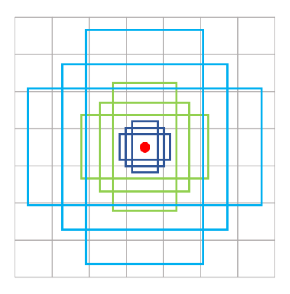
The regional proposal network uses anchor boxes to get the suggestion boxes of the feature map. Faster-RCNN uses three sets of rectangular boxes with different length-width ratios (2:1, 1:1, 1:2), and each set uses three fixed-size rectangular boxes with different scales (128, 256, 512) to stack at each pixel on the feature map, as shown in Figure 2. Then, each box was compared with ground truth box to calculate the intersection over union (IOU). The box with larger IOU than the large preset threshold is demarcated as foreground, and the box with smaller IOU than the small preset threshold is demarcated as background. Both the boxes with IOU between the two thresholds and the overflow boundary were directly discarded. Finally, we got the suggestion box to train the region proposal network (RPN).

The introduction of anchor boxes have brought many advantages. By setting different scales, all the targets can be covered as far as possible, while reducing the calculation amount and greatly reducing the difficulty of subsequent regression algorithm optimization.

2.1.2. Network Architecture

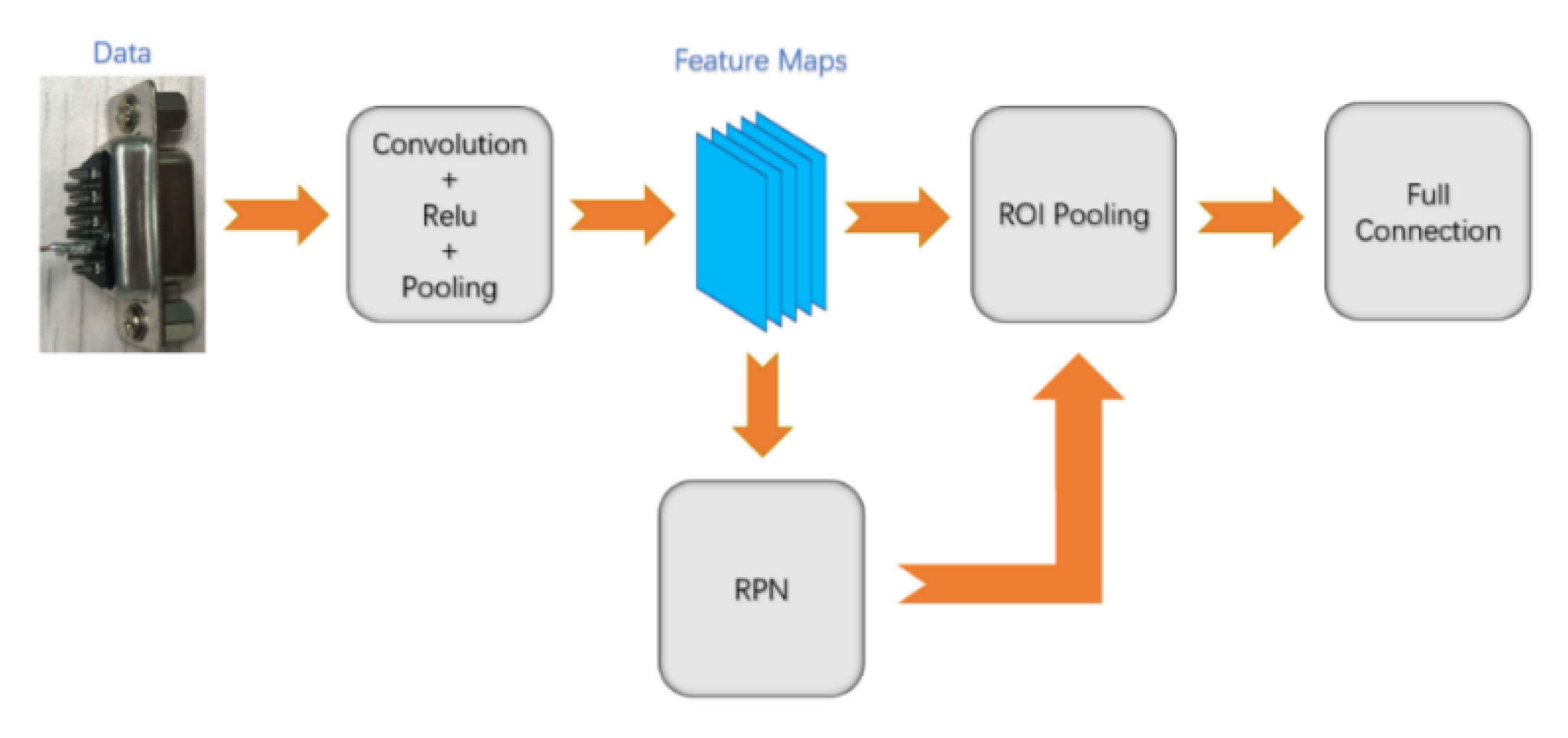
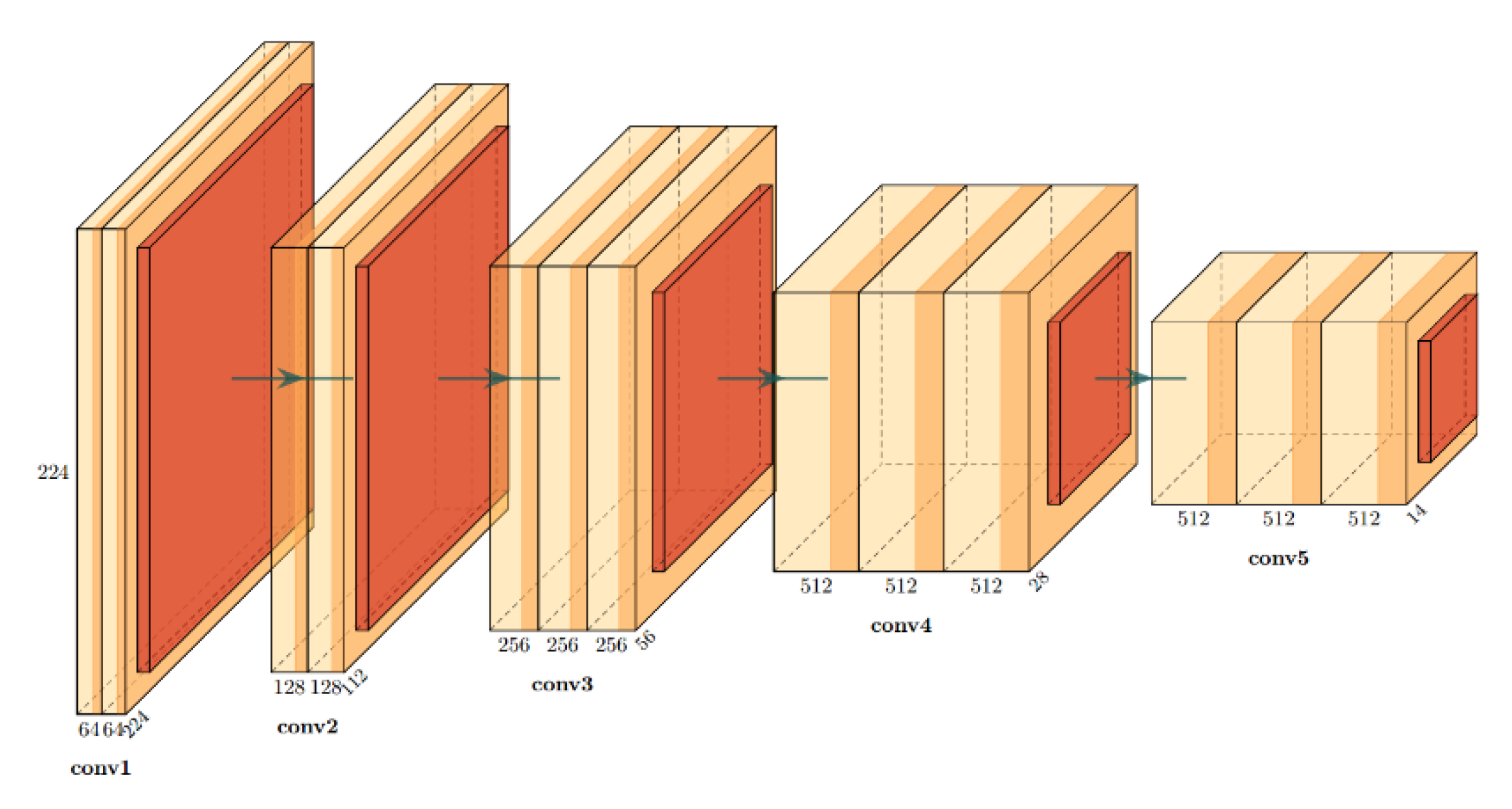
Faster-RCNN can be divided into four modules, including feature extraction module, regional proposal network (RPN) module, ROI pooling, and target classification and positioning module. The overall structure of the algorithm is shown in Figure 3. Currently, the released code of Faster-RCNN usually takes the convolution-pooling part of VGG-16 as the feature extraction module.

The feature extraction module firstly resizes the input data of any scale to a fixed scale (the long side of the image shall not be greater than 1000, and the short side of the image shall not be greater than 600), then extracts the data features through a set of convolution-ReLU-pooling layers, and generates n-dimensional feature map (512-dimensional feature map is generated by VGG-16 network). VGG-16 feature extraction network is shown in Figure 4.

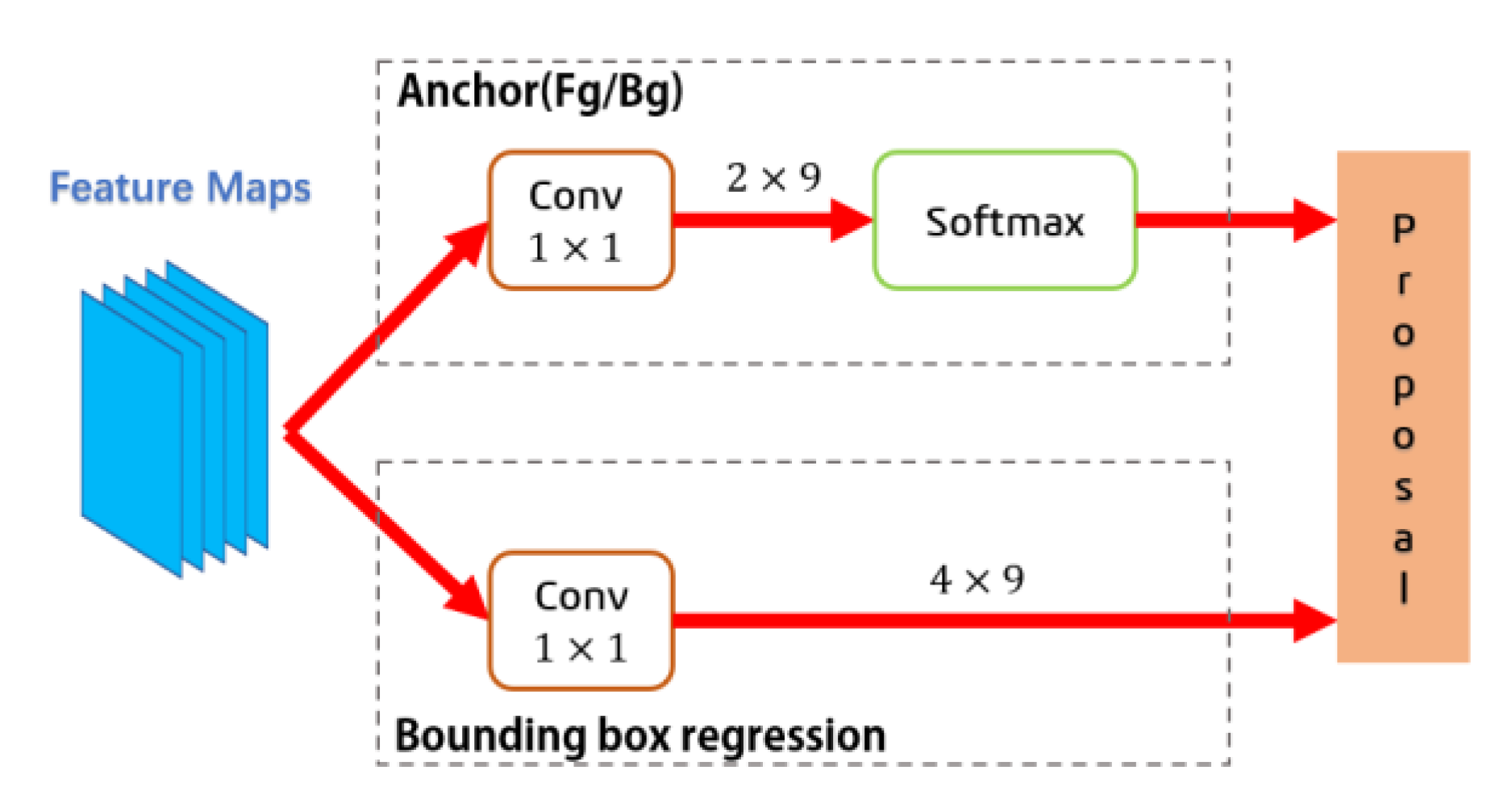
RPN uses anchor boxes to create rectangular boxes for each pixel on the feature map, assigns labels through the IOU value calculated with the ground truth boxes, and uses non-maximum suppression algorithm to eliminate overlapping boxes. The reserved foreground or background boxes will be assigned six variables, including four scale variables (x, y, w, h) and two label variables (Fg, Bg). The softmax algorithm is then used to calculate the target probability score for each box. The box regression algorithm uses four parameters to complete the regression of each anchor box, so that the proposed box is closer to the actual position. The algorithm process of RPN is shown in Figure 5.

The ROI pooling integrated feature maps and the proposal boxes generated by RPN, and proposal feature maps were calculated and generated. As the size of the proposal box is different, the dimension of input variables should be fixed when the subsequent full connection layer is used for classification. Therefore, Faster-RCNN uses ROI pooling to divide the proposal feature maps into seven equal parts horizontally and vertically, and performs the maximum pool on each square, so that the final size of each proposal feature map is 7 × 7.

The target classification and positioning module uses the full connection layer and softmax algorithm to categorize each proposal feature map, and output the probability vector. At the same time, bounding box regression is used again to obtain the positional offset of each suggested feature map and to generate a more accurate detection box.

2.1.3. Loss Function

The loss function of Faster-RCNN mainly consists of two parts, including the loss function of RPN and the loss function of RCNN, and each loss function includes the classification loss and the regression loss. The classification loss $L_{cls}(\ast )$ was calculated using cross-entropy, and the regression loss $L_{reg}(\ast )$ was calculated using smooth-L1. RPN loss function and RCNN loss function are shown in Equations (1) and (2).

$$L_{RPN}\left(\left\{p_i\right\},\left\{t_i\right\}\right)=\frac{1}{N_{cls}}{\displaystyle \sum }_i{L}_{cls}\left(p_i,p_i^{*}\right)+\lambda \frac{1}{N_{reg}}{\displaystyle \sum }_i{p}_i^{*}{L}_{reg}\left(t_i,t_i^{*}\right)$$

(1)

where $N_{cls}$ represents the number of images in each minibatch, and $N_{reg}$ represents the number of anchor boxes in each minibatch, with a difference for nearly 10 times. Therefore, in order to balance the classification loss and regression loss, a coefficient $\lambda =10$ is added in the regression loss function section. $p_i$ represents the category score vector of the proposal box, $p_i^{*}$ represents the label of the proposal box, $t_i$ represents the position parameter of the proposal box, $t_i^{*}$ represents the position parameter of the proposal box, and $i$ represents each annotation box.

$$L_{RCNN}\left(p,u,t^u,v\right)=L_{cls}\left(p,u\right)+L_{reg}\left(t^u,v\right)$$

(2)

where $p$ represents the score of the category predicted by the network, $u$ represents the score of the ground truth, $t^u$ represents the coordinate of the ground truth, and $v$ represents the coordinate of the predicted box.

2.2. Important Improvements

In order to detect solder joint defects, we welded 625 solder joint samples and completed the images collection. In terms of algorithm, we used the open source TensorFlow version of Faster-RCNN algorithm on the network to train and test the test images. We found that the automatic detection of solder joint defects could not be realized with obvious effect, and a large number of undetected solder joint defects would lead to insufficient product performance. After comprehensive analysis, we believe that the main reasons are as follows: 1. There are too few training samples, so the network does not converge well after training; 2. The depth of the model is insufficient, and the ability to extract solder joint features of the connector is insufficient; 3. The scales of the default anchor do not match the size of the solder joint, and the positioning is not accurate, so the features are not fully learned by the network. Therefore, the following three improvement strategies are proposed, including data augmentation, k-means clustering to generate anchor boxes, and transfer learning with ResNet-101.

2.2.1. Data Augmentation

In this paper, 625 solder joint sample images were collected, including five types of qualified solder joints, multi-tin solder joints, less-tin solder joints, connected welding solder joints, and tin tip solder joints. Among them, 100 images were randomly selected as test images, and the remaining 525 images were used as training data, including 336 images of training set, 84 images of verification set and 105 images of test set. The deep neural network contains a large number of hidden layers and weights, and the data amount is too small to adjust the weights, which leads to the under-fitting of the model after training, thus affecting the accuracy of the model, and the actual detection effect will be poor. However, the limited welding capacity makes it difficult to continue expanding the data volume beyond the existing solder spot samples, and this is leading to the use of data augmentation to realize the expansion of the data set.

Data augmentation is a means of applying a set of basic forms of image processing to generate new images and, at the same time, corresponding label files for deep network training, usually involving rotation, mirror flipping, random shearing, brightness switching, contrast switching, etc. They can increase the data set. At the same time, different transformation eliminates the effect of target’s position, brightness, color and other properties in the image, so that the model can better recognize the target and improve the accuracy of the model. The data augmentation technology employed in this paper includes left-right flipping, up-down flipping, diagonal flipping, random brightness, and random contrast, and the results of this change are shown in Figure 6. In order to improve the robustness of the model, all transformations are random.

After data augmentation, the training data in this paper were expanded from 525 images to 1654 images, including 1059 images in the training set, 265 images in the validation set and 330 images in the test set.

2.2.2. K-Means Clustering Generates Anchor Boxes

The size of anchor boxes in the Faster-RCNN algorithm refers to the target size in VOC 2007 and VOC 2012 data set. The generated boxes can cover most of the targets, and a more accurate suggestion box can be obtained through regression. However, the size of the pin in the connector is small in the image. Although the official anchor box can get a more accurate suggestion box by training the regression coefficient, the adjustment scale is too large, which is not conducive to convergence. Therefore, k-means clustering is adopted in this paper to analyze all training data and obtain a set of anchor boxes with more appropriate scale. K-means clustering pseudo code is shown in

Table 2. K-means clustering pseudo-code.

Ground Truth Boxes: $\left\{\left({\mathit{w}}_{\mathit{i}}^{*},{\mathit{h}}_{\mathit{i}}^{*}\right)\right\}, \mathit{i}\in \left[1, \mathit{N}\right]$

Initialize k clustering centers: $\left\{\left(w_j,h_j\right),j\in \left[1,k\right]\right\}$ Iteration: stop if the change of new clustering centers is smaller than threshold. for$i$ in range ($N$): for $j$ in range ($k$): $d_i\left(j\right)=1-IOU\left(\left(w_i^{*},h_i^{*}\right),\left(w_j,h_j\right)\right)$ $cls\left(i\right)=Index(\underset{j\in \left[1,k\right]}{min} d_i\left(j\right))$ Calculate new $k$ clustering centers: $w_j^{\prime }=\frac{1}{N_j}{\displaystyle \sum }{w}_i^{*}\left(j\right),h_j^{\prime }=\frac{1}{N_j}{\displaystyle \sum }{h}_i^{*}\left(j\right),i\in \left[1,N\right],j\in \left[1,k\right]$

.

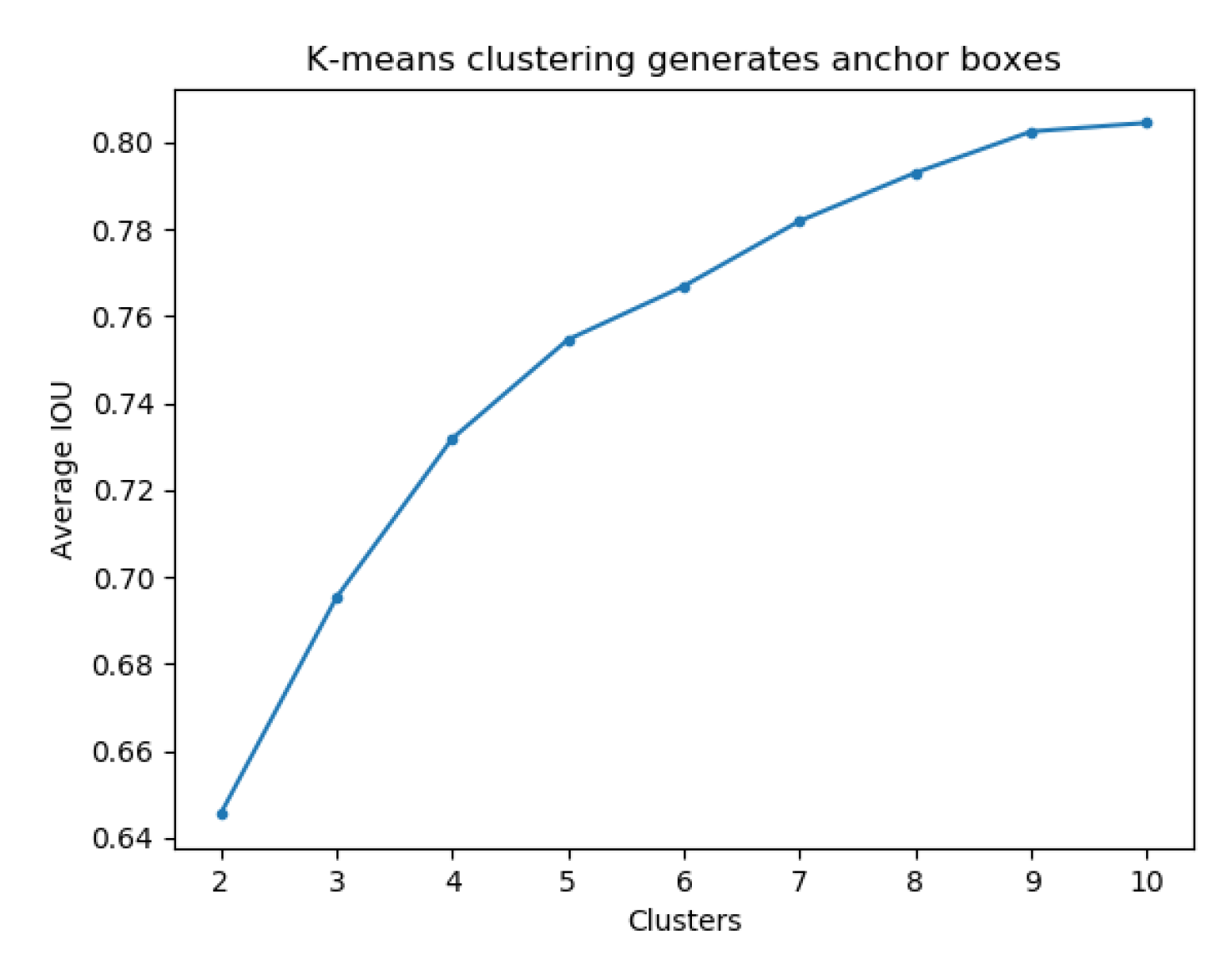
Anchor boxes generated by k-means clustering are more in line with the actual size of detection targets compared with the preset anchor boxes based on experience, which is conducive to regression and obtaining a suggestion box with higher accuracy. Generally speaking, the larger a k value is, the more anchor boxes are generated and the higher the accuracy is. However, when k value is increased to a certain extent, the accuracy is basically unchanged, while too many suggestion boxes will greatly reduce the computational efficiency of the network. Therefore, the value range of k is generally defined in [2,10]. The average Intersection-over-Union (IOU) of anchor boxes generated by k-means clustering under different k values are shown in Figure 7.

2.2.3. Transfer Learning with ResNet-101

In the target detection task, the depth of the convolutional neural network is usually up to dozens or even hundreds of layers due to the complexity of the shape, color, and other characteristics of the target in the image. However, the deeper layer is not conducive to the parameter optimization of the network, and gradient explosion or gradient disappearance are likely to occur during the training process [25]. Although batch-norm, random gradient descent and other algorithms can be used to achieve a certain degree of optimization, the effect is not obvious. Therefore, in 2015, He proposed a new network structure unit, which is called the residual unit. Meanwhile, in 2016, He improved the residual unit to make it easier to train and increase its generalization ability [26]. The remaining units can be divided into 2 layers of remaining units and 3 layers of remaining units, as shown in Figure 8. The deep convolutional network consisting of the remaining units is called ResNet.

The residual unit changes the operation mode of the traditional convolutional network, in which, the final value obtained by convolutional layer and ReLU is shown in Equation (3).

$$H\left(x\right)=F\left(x\right)+x$$

(3)

where $F\left(x\right)$ is the difference between the output $H\left(x\right)$ and the input $x$, namely the residual. In an ideal situation, when the network reaches a certain depth, if the network state is already optimal, $F\left(x\right)$ should be set as 0, which is equivalent to the output $H\left(x\right)$ of the residual unit as $x$, so that the current depth network does not degrade, which ensures the accuracy of the deep network model.

ResNet has a variety of network structures, which can be divided into 18, 34, 50, 101, and 152 layers according to the convolutional layer depth. The residual units contained in different network structures are slightly different, as shown in

Table 3. ResNet-N network structure and accuracy.

Layer Name	Output Size	18-Layer	34-Layer	50-Layer	101-Layer	152-Layer
conv1	$112\times 112$	7 × 7, 64, stride 2
conv2_x	$56\times 56$	3 × 3 max pool, stride 2
		$\left[\begin{array}{c}3\times 3, 64\\ 3\times 3, 64\end{array}\right]\times 2$	$\left[\begin{array}{c}3\times 3, 64\\ 3\times 3, 64\end{array}\right]\times 3$	$\left[\begin{array}{c}1\times 1, 64\\ 3\times 3, 64\\ 1\times 1, 256\end{array}\right]\times 3$	$\left[\begin{array}{c}1\times 1, 64\\ 3\times 3, 64\\ 1\times 1, 256\end{array}\right]\times 3$	$\left[\begin{array}{c}1\times 1, 64\\ 3\times 3, 64\\ 1\times 1, 256\end{array}\right]\times 3$
conv3_x	$28\times 28$	$\left[\begin{array}{c}3\times 3, 128\\ 3\times 3, 128\end{array}\right]\times 2$	$\left[\begin{array}{c}3\times 3, 128\\ 3\times 3, 128\end{array}\right]\times 4$	$\left[\begin{array}{c}1\times 1, 128\\ 3\times 3, 128\\ 1\times 1, 512\end{array}\right]\times 4$	$\left[\begin{array}{c}1\times 1, 128\\ 3\times 3, 128\\ 1\times 1, 512\end{array}\right]\times 4$	$\left[\begin{array}{c}1\times 1, 128\\ 3\times 3, 128\\ 1\times 1, 512\end{array}\right]\times 8$
conv4_x	$14\times 14$	$\left[\begin{array}{c}3\times 3, 256\\ 3\times 3, 256\end{array}\right]\times 2$	$\left[\begin{array}{c}3\times 3, 256\\ 3\times 3, 256\end{array}\right]\times 6$	$\left[\begin{array}{c}1\times 1, 256\\ 3\times 3, 256\\ 1\times 1, 1024\end{array}\right]\times 6$	$\left[\begin{array}{c}1\times 1, 256\\ 3\times 3, 256\\ 1\times 1, 1024\end{array}\right]\times 23$	$\left[\begin{array}{c}1\times 1, 256\\ 3\times 3, 256\\ 1\times 1, 1024\end{array}\right]\times 36$
conv5_x	$7\times 7$	$\left[\begin{array}{c}3\times 3, 512\\ 3\times 3, 512\end{array}\right]\times 2$	$\left[\begin{array}{c}3\times 3, 512\\ 3\times 3, 512\end{array}\right]\times 3$	$\left[\begin{array}{c}1\times 1, 512\\ 3\times 3, 512\\ 1\times 1, 2048\end{array}\right]\times 3$	$\left[\begin{array}{c}1\times 1, 512\\ 3\times 3, 512\\ 1\times 1, 2048\end{array}\right]\times 3$	$\left[\begin{array}{c}1\times 1, 512\\ 3\times 3, 512\\ 1\times 1, 2048\end{array}\right]\times 3$
	$1\times 1$	average pool, 1000-d fc, softmax
FLOPs		$1.8\times {10}^9$	$3.6\times {10}^9$	$3.8\times {10}^9$	$7.6\times {10}^9$	$11.3\times {10}^9$
Top-1 error		27.88%	25.03%	22.85%	21.75%	21.43%

. ResNet-18 and ResNet-34 are composed of 2-layers residual units, while ResNet-50, ResNet-101, and ResNet-152 are composed of 3-layers residual units.

At present, ResNet is widely used due to its remarkable parameter optimization ability in training [27,28,29,30]. In this paper, considering the accuracy of defect detection and actual computing ability, the convolution part of ResNet-101 was selected as the feature extraction module, and the original VGG-16 was replaced to improve the accuracy of the final detection results.

3. Results

In this paper, we chose the open-source version of TensorFlow Faster-RCNN on GitHub as the basic algorithm framework. In terms of hardware, Inter Core I7-8750h CPU and Nvidia GTX 1050Ti 8G GPU were used to achieve efficient operation rate. As for the data, 625 solder joint images were collected, including five types, namely qualified, multi-tin, less-tin, connected welding, and tin tip. A total of 100 images were randomly selected as the test images, and the remaining 525 images were expanded through the data augmentation and made into the training set, verification set and test set. In terms of network model parameters, the maximum steps of training were 30000, the batch-size was selected as 256, and the learning rate was selected as 0.001.

In the experiment, we first used the initial training set to train the original version of Faster-RCNN, and proposed three improvement strategies by analyzing the results. Subsequently, we used the enhanced data set for comparison experiments to verify the effectiveness of k-mean clustering, and used ResNet-101 to generate anchor boxes and transfer learning, respectively. Finally, we fused all the improved algorithms and completed the task of connector solder joint defect detection. By comparing and analyzing the experimental results, it is proved that the algorithm proposed in this paper is efficient and feasible for the detection of connector solder joint defects.

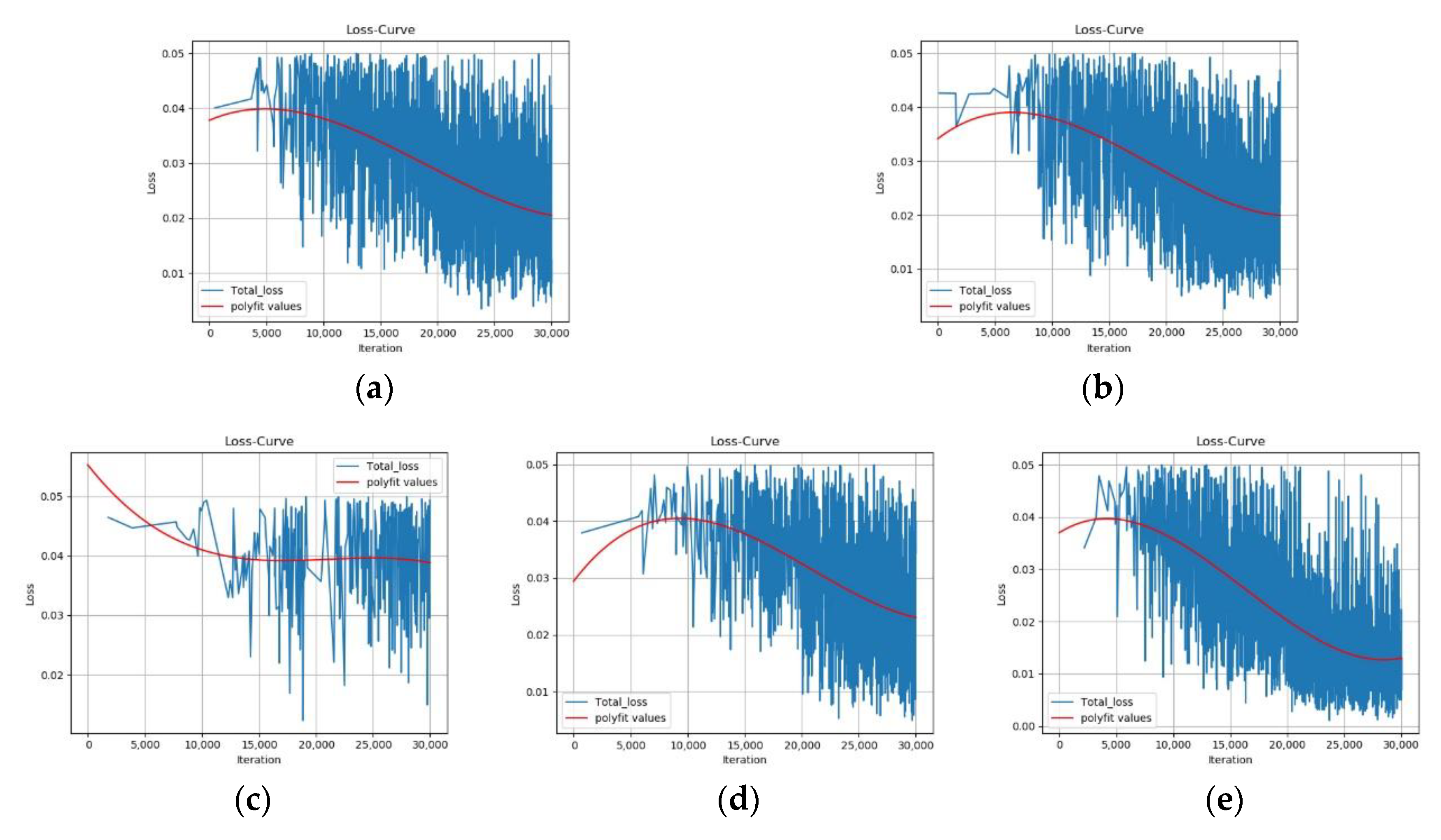
In the original version of Faster-RCNN, 9 fixed anchor boxes were selected, which were obtained through the comprehensive analysis of the target scale of Pascal VOC data set. Although the anchor boxes generated can contain most of the areas of the solder joint defect target in this paper, the offset coefficient in the regression algorithm is too large compared to the boxes with closer scales, resulting in the inaccurate position of the calculated proposals. This problem is particularly evident at the beginning of training, as shown in Figure 9a. The proposal loss obtained after using k-means clustering to generate anchor boxes algorithm is shown in Figure 9b. If the loss mutation caused by insufficient batch size (GPU memory limit) is not taken into account, it can be seen that the concussion range of loss in the early training period is reduced to a certain extent after using k-means clustering generates anchor boxes algorithm, and the final loss of network model has no obvious change.

A deep learning target detection model usually used the mAP as an index to measure the detection accuracy. By gradually reducing the threshold value of sample classification, the recall rate and corresponding precision of samples under each threshold value were calculated, and the precision-recall curve was drawn, and the area of the curve and the coordinate axis was mapped. The closer the mAP of a network model approaches 1, the higher the accuracy of the current network model will be.

Table 4. mAP of original network and different training model.

	mAP
VGG-16	0.8364
VGG-16 + data augmentation 1	0.8554
VGG-16 + data augmentation + k-means clustering 2	0.8670
ResNet-101 + data augmentation 3	0.9337
This paper	0.941

^1,2,3 Training model using different improved algorithm.

and

Table 5. Detection accuracy of 5 solder joint types and mean detection accuracy.

	Qualified	Multi-tin	Less-tin	Connected Welding	Tin Tip	Mean Accuracy
Original	60%	95%	65%	90%	75%	77%
Training model 1	65%	90%	70%	95%	70%	78%
Training model 2	70%	85%	70%	95%	80%	80%
Training model 3	90%	95%	90%	95%	85%	91%
This paper	90%	95%	95%	100%	90%	94%

^1,2,3 Training model using different improved algorithm. Corresponds to the number in Table 4.

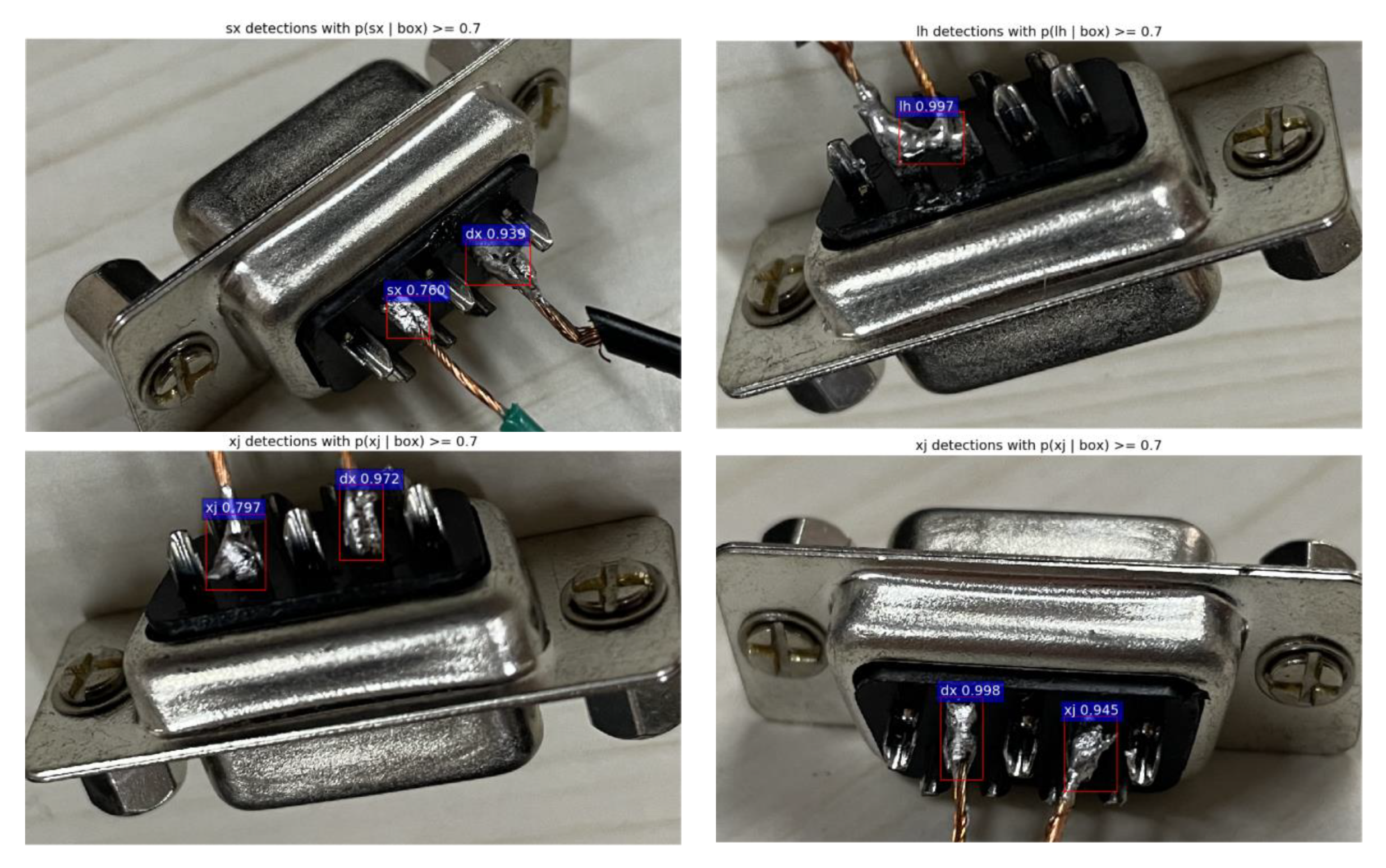
list the mAP and detection accuracy of the network model under different conditions, respectively. Figure 10 and Figure 11 show the precision-recall curves of different training models and the total loss curves in the training process respectively. Figure 12 lists some of typical detection results of the method proposed in this paper. According to the experimental results, the model mAP and detection accuracy are improved to some extent after the training set is enhanced. In the case of using enhanced training set, k-means clustering generates anchor boxes and transfer learning with ResNet-101 both improve the accuracy of model mAP and detection accuracy, among which ResNet-101 plays a more obvious role. The final mAP and detection accuracy of the algorithm proposed are 0.941 and 94%, respectively, which significantly improves the effect of the original Faster-RCNN under the same training set.

4. Discussion

In this paper, the algorithm of Faster-RCNN was improved. The five transformation modes of left-right flipping, up-down flipping, diagonal flipping, random brightness, and random contrast were used in the data set to solve the problem of small amount of data in the original data set and avoid the situation of under-fitting during network model training. According to the generation mode of anchor boxes in RPN, this paper proposed to cluster the data sets using k-means clusters, analyzed the average IOU of anchor boxes generated by clustering algorithm in the case of different k values, and then selected appropriate clusters number to generate anchor boxes, which improved the positioning accuracy of proposals. Given the insufficiency of feature extraction network for connector’s solder joint defect feature extraction capability, the convolutional neural network with deeper layers is needed. In addition, considering that the deepening of the network may cause gradient explosion and reduce the accuracy of the model, this paper proposed to replace the VGG-16 with ResNet-101. After network replacement, the algorithm mentioned in this paper has enhanced its own ability to extract solder joint defect characteristics of connectors, and the network model has higher accuracy and stability.

After comparing and analyzing the actual detection capability and model precision of different algorithms, we find that the algorithm proposed in this paper is superior to the original Faster-RCNN in all aspects. The mAP of the algorithm increased from 0.8554 to 0.941, increasing by 8%. The final top-1 accuracy rate increased from 78 to 94%, with an improvement of 16%. Nevertheless, 94% of top-1 accuracy has been able to meet the needs of industrial detection.

We hope to detect the solder joint defects automatically with machine vision, so the algorithm proposed can only detect the solder joint image collected by the optical camera, but cannot detect the defects such as cracks or bubbles inside the solder joint. Currently, there are various types of connectors used in electronic products, and the sample used in this paper is only D-type data interface connector with 9 pins. However, the defect type and appearance of solder joint of connector are basically the same because the shape of welding cup of different connector is similar. Therefore the improved Faster-RCNN algorithm proposed in this paper can still obtain similar high accuracy rate, for the detection of solder joint defects in different connectors.

In the industry, there are many kinds of defects in connector solder joints. This paper only took 4 typical defect types and qualified solder joints as examples to train the model in this paper, it is still a long way to go in terms of ultimate practicality. Meanwhile, due to the lack of computing power, the algorithm of batch size 256 can see the loss jumping in the training process. The reason is that the smaller batch size does not match the images of more data sets, so the batch normalization effect of each batch of images is poor, which affects the model training and reduces the test accuracy to a certain extent. Therefore, in the following research, we will increase the types and images of solder joint defects, and at the same time consider more optimized training methods, so as to increase the algorithm’s ability to detect more kinds of solder joint defects on the premise of ensuring high accuracy and at the same time reduce the detection cost.

5. Conclusions

This paper has captured images of connectors containing the five solder joint types, achieved data expansion and trained, verified, and tested them with data augmentation. After training, the algorithm proposed in this paper has been verified by comparison experiments to be more accurate in the detection of solder joint defects. The main contributions of this paper are as follows: First, there are few studies on solder joint quality inspection at present, and most of them are detected by workers’ eyes during welding. The method proposed in this paper has obtained high detection accuracy, which provides a new way of thinking for solder joint quality detection of connectors. Secondly, a data set containing five solder joint types is produced to train the solder joint quality inspection network. At the same time, the data set will be filled in the following research process to enable the network to detect more connector solder joint defect types; Thirdly, the network model performance and the final detection accuracy have been significantly improved after optimization of the algorithm proposed in this paper. Therefore, the optimization method can also provide a new optimization strategy for solving similar target detection problems.