Partial Least Squares Improved Multivariate Adaptive Regression Splines for Visible and Near-Infrared-Based Soil Organic Matter Estimation Considering Spatial Heterogeneity

Abstract

Under the influence of complex environmental conditions, the spatial heterogeneity of soil organic matter (SOM) is inevitable, and the relationship between SOM and visible and near-infrared (VNIR) spectra has the potential to be nonlinear. However, conventional VNIR-based methods for soil organic matter estimation cannot simultaneously consider the potential nonlinear relationship between the explanatory variables and predictors and the spatial heterogeneity of the relationship. Thus, the regional application of existing VNIR spectra-based SOM estimation methods is limited. This study combines the proposed partial least squares–based multivariate adaptive regression spline (PLS–MARS) method and a regional multi-variable associate rule mining and Rank–Kennard-Stone method (MVARC-R-KS) to construct a nonlinear prediction model to realize local optimality considering spatial heterogeneity. First, the MVARC-R-KS method is utilized to select representative samples and alleviate the sample global underrepresentation caused by spatial heterogeneity. Second, the PLS–MARS method is proposed to construct a nonlinear VNIR spectra-based estimation model with local optimization based on selected representative samples. PLS–MARS combined with the MVARC-R-KS method is illustrated and validated through a case study of Jianghan Plain in Hubei Province, China. Results showed that the proposed method far outweighs some available methods in terms of accuracy and robustness, suggesting the reliability of the proposed prediction model.

1. Introduction

Soil organic matter (SOM) content is significantly relevant to soil fertility, biological productivity, and agricultural sustainable development [1,2]. Accurate prediction of SOM content is of great significance for land management [1,3]. Extensive studies have fully affirmed the capability of SOM prediction methods based on visible and near-infrared (VNIR) spectra [4,5]. However, the function relation between SOM content and VNIR spectra should be established because of the strong soil spatial heterogeneity under the influence of complex environmental conditions. In addition, the formation, variation, and decomposition of SOM are generally influenced by various factors, and the VNIR spectra are comprehensively related to various soil properties; hence, the relation of SOM content to VNIR spectra is complex with high nonlinearity [6,7]. Therefore, further exploration of VNIR spectra-based SOM prediction models is needed to improve simulation and prediction accuracies.

An extensive literature review demonstrates that previous methods for predicting soil properties can be categorized into linear and nonlinear prediction methods. For example, multiple linear regression (MLR), partial least squares (PLS) regression, and geographic weighted regression (GWR) are typical linear prediction methods. These methods have been extensively used in many previous studies because they are easily accessible in most software packages [4]. A common characteristic of these prediction methods is that they assume, either explicitly or implicitly, a linear relationship among the analyzed data sets. A nonlinear relationship, however, is prevalent in practice between SOM content and VNIR spectra. Thus, a series of nonlinear prediction methods has been proposed to estimate nonlinear relationships, including, but not limited to, local weighted regression (LWR) [8,9], artificial neural network [10,11], and support vector machine (SVM) methods [12,13]. Although these methods can efficiently determine nonlinear relationships in certain situations, they lead to models based on global optimization and disregard the spatial heterogeneity of the nonlinear relationship. This underlying principle will cause the accuracy of existing methods to easily change with different samples and have difficulty for application to other regions. Therefore, nonlinear estimation methods considering spatial heterogeneity are needed for SOM content prediction.

The multivariate adaptive regression spline (MARS) method is a nonlinear prediction method that considers the effects of local difference. The MARS method is the expansion of splines, thereby providing immense flexibility by automatically determining the splines (i.e., the number of basis functions (BFs) and locations of knots) without human interference. This method has been successfully applied to various fields, such as geotechnical engineering and soil liquefaction assessment [14,15,16]. The MARS method has proven to be advantageous due to its adaptation to nonlinear relationships and to its adaptive model construction process, while considering the natural local difference in the training data sets. These characteristics of the MARS method indicate its considerable potential to represent the relationships between VNIR spectra and SOM content. Although tracked records of the application of the MARS model to soil property prediction are available in literature [11,17], these records are not well received. The possible reason may be that most of the applications implicitly or explicitly consider the explanatory variables as mutually independent, which is often not the case in reality. In fact, the VNIR spectra of soil samples are the comprehensive representation of soil properties, and thus multicollinearity inevitably exists. As such, multicollinearity should be removed to obtain relatively independent variables when constructing a MARS model. The multicollinearity-removing strategy from PLS regression is verified to be beneficial by reducing the dimensionality, considering the high dimensionality and correlated representations [4,18]. Therefore, this research proposes the utilization of partial least squares regression to remove multicollinearity and obtain extensive information on the explanatory variables; the resultant principal components (PCs) from the PLS regression are used as a replacement for the original explanatory variables to construct a MARS model, thereby overcoming the weakness of the available MARS model for prediction of soil properties. For simplicity, the entire process is referred to as the partial least squares–based multivariate adaptive regression spline (PLS–MARS) method herein. The proposed PLS–MARS method can effectively represent the nonlinear relationship between the data with local difference and numerous variables, as will be discussed in Section 3.

The accuracy of the prediction model relies significantly on calibrated samples. Underrepresentation of calibrated samples will lead to a biased prediction model due to soil spatial heterogeneity. However, preceding studies (e.g., [8,9,11,12]) focused exclusively on developing new prediction models for estimating soil properties, disregarding the influence of the calibration sets on the reliability of the prediction models. In particular, the calibration sets in most of these studies were selected randomly or from several available methods, such as the concentration gradient method (C method) [19,20]. The prediction model may be biased if inappropriate calibration sets are adopted [3]. Hence, reasonable calibration sets should be selected before they are applied to construct prediction models. Accordingly, our newly developed multi-variable analysis method (i.e., regional multi-variable associate rule mining and Rank–Kennard-Stone (MVARC-R-KS) method) [3] was adopted to select calibration sets in the current study (see Subsection III-A for elaboration). The MVARC-R-KS method was used due to the following two reasons. (1) This method is effective in enhancing the accuracy of linear prediction methods, such as PLS regression (Wang, Chen, Guo and Liu [3]), thereby providing the confidence to extend it for nonlinear prediction methods (e.g., the proposed PLS–MARS method in this study). (2) The MVARC-R-KS method can consider multiple influential factors (e.g., chemical component, spectrographic information, and environmental factors) and select a representative calibration set, which makes the VNIR-spectrum–based SOM prediction model calibrated from such a calibration set as to be an extensively applicable one [3]. Three commonly used calibration set selection methods, namely, component concentration representative methods (e.g., the C method [19,20]), spectrum representative methods (e.g., the Kennard–Stone (KS) method [21]), and component concentration and spectrum representative methods (e.g., the Rank–Kennard-Stone (Rank–KS) method [22]), are also utilized and compared with the MVARC-R-KS method to investigate their influences on the prediction models and further verify the effectiveness of the proposed method. To the best of our knowledge, such a systematic comparison of the influences of different calibration set selection methods on the performance of SOM prediction models, particularly nonlinear prediction models, such as the proposed PLS–MARS model herein, appears to be original. This comparison is expected to guide the calibration set selection for a specific prediction model in the future.

The remainder of the paper is structured as follows. The study area and materials for this study are introduced in Section 2. The calibration set selection methods and the proposed PLS–MARS prediction method are described in Section 3. Experiments on the simulated data set and real application are discussed in Section 4, illustrating and validating the proposed method. The principal contributions and observations of this study are discussed in Section 5. Section 6 concludes this research.

2. Study Area and Materials

2.1. Study Area

Sampling was done in Jianghan Plain in Hubei Province, China. Jianghan Plain is an important agricultural region because of the humid climate and fertile soil. However, in recent years, the ecological system of the plain has become unstable, and the SOM content has decreased due to long-term agricultural activities. Therefore, estimating the SOM content with high accuracy in this plain is necessary and beneficial to land resource management. To this end, 260 topsoil samples (i.e., 0 cm to 30 cm; see Figure 1) were obtained from this area in June 2014. The samples were taken at least 100 m apart from one another. All samples were partitioned into two parts for chemical study and spectral measurement.

2.2. SOM Content and Spectral Measurement

SOM content was measured by following the analysis and calculation methods in literature [3,23]. An ASD FieldSpec3 portable spectral radiometer was used to measure spectral reflectance, which ranged from 350 nm to 2500 nm with a sampling interval from 1.4 nm to 2 nm. The measurement procedures were carried out in the dark to decrease the interference of external light. The light source was from a standardized white halogen light, which had a 45° incident angle and was at a distance of 45 cm.

3. Methods

VNIR spectra-based SOM content prediction generally consists of the following three parts. Part 1 is the spectral preprocessing. Spectral reflectance is unavoidably impacted by random noises, baseline drift, and scattering effects because of the influence of error from the experimental instruments and ambient noises; thus, the stability of the constructed VNIR-spectrum–based prediction model is affected [3]. Hence, spectral preprocessing is a prerequisite for the construction of the prediction model, which will be detailed in Section 3.1. In part 2, the representative calibration set is selected using methods such as the MVARC-R-KS method [3], which will be detailed in Section 3.2. Part 3 aims to build an SOM prediction model based on the VNIR spectra, such as by using typical prediction methods and the proposed PLS–MARS method, which will be elaborated in Section 3.3.1. Lastly, in Section 3.3.2, the accuracy of the constructed prediction model is evaluated by several assessment indices, as will be described in Section 3.3.2.

3.1. Spectral Preprocessing

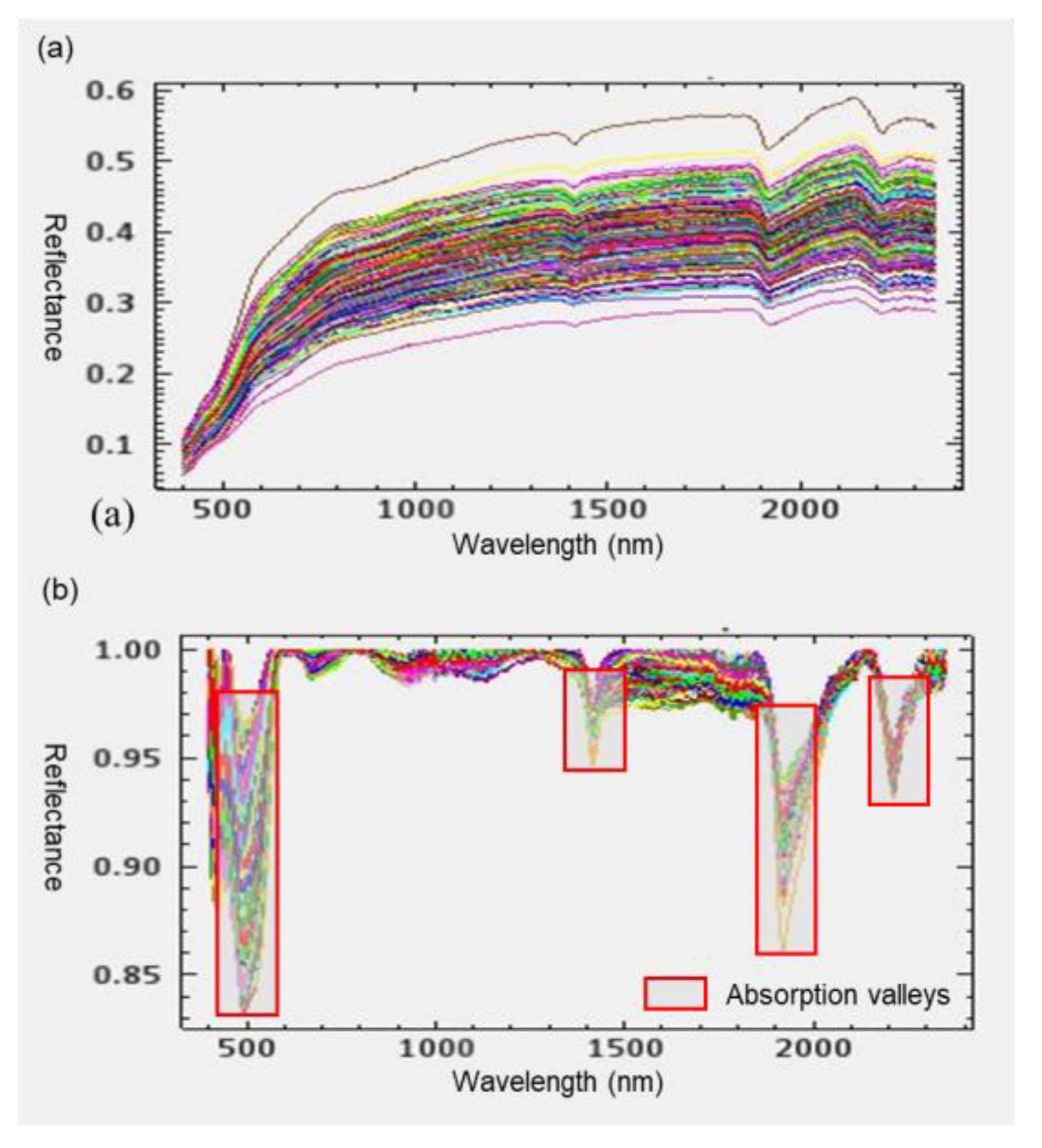
According to the characteristics of the spectra, spectral preprocessing was conducted as follows. The spectra ranging from 400 mm to 2350 mm was retained to reduce the interference of noises (Liu et al., 2014b; Liu et al., 2016) (Figure 2a). In addition, continuum removed spectral curves exhibited several diminutive absorption valleys (Figure 2b), which could interfere with the prediction based on the VNIR spectra. Hence, Savitzky–Golay (SG) smoothing was used to denoise this interference. Furthermore, multiplicative scatter correction (MSC) and mean center (MC) operations were utilized to reduce the influence of the unavoidable scattering. In short, the spectra were preprocessed successively through SG smoothing, MSC operation, and MC operation.

3.2. Calibration Set and Validation Set Selection Methods

The MVARC-R-KS method [3] aimed at adaptively selecting the calibration set through multivariate analysis. The procedure of selecting the calibration set using the MVARC-R-KS method comprised two phases [3]. Phase 1 initially mined the clustering distribution zones using the MVARC method, which integrated the a priori algorithm, a density-based clustering algorithm, and the Delaunay triangulation [3]. The association between the SOM content and VNIR spectra may vary according to location and surrounding environment, contributing to the generally strong spatial variability of soil samples. Hence, to open out the spatial heterogeneity of soil samples, environmental variables and SOM content were set as input data for the MVARC method. The spatial heterogeneity of soil samples was checked by Moran’s I; results are given in

Table 1. Moran’s I index and z-score of data related with prediction models calibrated by different calibration set selection methods.

Prediction Model	Selection Method	Original Data		Predicted Data		Residuals
		I	Z-Score	I	Z-Score	I	Z-Score
Partial least squares–based geographic weighted regression (PLS–GWR)	Concentration gradient (C) method	1.15	6.33	1.06	5.83	0.01	0.20
	Kennard-Stone (KS) method	1.28	5.87	1.15	5.23	−0.07	−1.27
	Rank–Kennard-Stone (Rank–KS) method	1.33	6.30	1.28	6.03	−0.10	−1.35
	Regional multi-variable associate rule mining and Rank–Kennard-Stone (MVARC-R-KS) method	1.39	6.17	1.24	5.49	−0.07	−0.96
Partial least squares–based multivariate adaptive regression (PLS–MARS)	C	1.15	6.33	1.03	5.69	−0.01	0.06
	KS	1.28	5.87	1.12	5.15	0.07	1.42
	Rank–KS	1.33	6.30	1.12	5.30	−0.01	0.01
	MVARC-R-KS	1.39	6.17	1.17	5.23	0.08	1.33

. Samples in the same cluster mined by the MVARC method were relatively similar with respect to the impact of the surrounding environment. In addition, the influence of environmental variables on SOM in clusters presented significant differences. Phase 2 utilized the Rank–KS algorithm [22] to select the calibration set from the clustering zones. The eventually selected calibration set was an internal component concentration and spectrum representations, as well as an external environment representation. In addition, the size of the calibration set was set as approximately 70% of the soil samples, and the remaining 30% of the samples were used as the validation set, referring to previous studies [23,24].

Apart from the MVARC-R-KS method, three commonly used calibration set and validation set selection methods––C method, KS method, and Rank–KS method––were utilized for comparison to verify the representation of the selected calibration set.

3.3. VNIR-Based Prediction Methods

According to the VNIR-based SOM predicting demands, the PLS–MARS method was proposed to effectively represent the nonlinear relationship between the data with local difference and numerous variables (see Section 3.3.1). To verify the effectiveness of the proposed PLS–MARS method, typical prediction methods, such as MLR, SVM, PLS, and GWR, were used to construct VNIR-based SOM prediction models. To realize a more comparative analysis with the proposed PLS–MARS method, the GWR method was also combined with PLS (named PLS–GWR) to construct a prediction model. Eventually, a series of evaluation indices was used to evaluate the simulation and prediction performance of the prediction models, which is described in detail in Section 3.3.2.

3.3.1. PLS–MARS Method

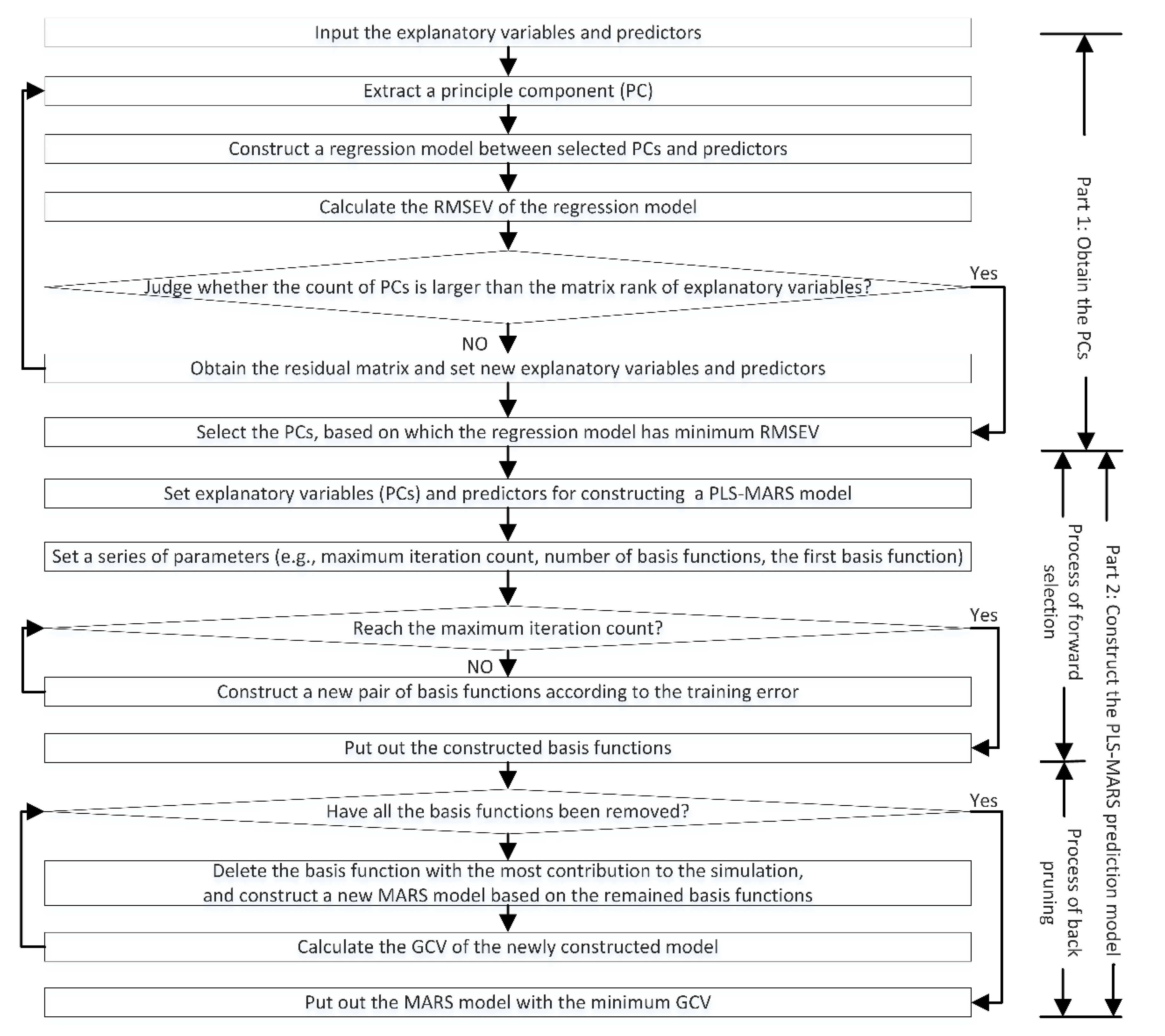
The PLS–MARS method is a combination of PLS and MARS methods that constructs a nonlinear prediction model with local regression. The flow of PLS–MARS comprises two parts (Figure 3). Part 1 removes the multicollinearity of the explanatory variables by obtaining PCs using a PLS regression method. Part 2 constructs the MARS model based on the predictors and PCs obtained in Part 1. The details of PLS–MARS are described as follows.

PCs were abstracted in Part 1. The explanatory variables and predictors were labeled as $E_0$ and $F_0$, respectively. The procedure of obtaining PCs was to abstract the PCs first. Thereafter, a series of PLS regression models based on the obtained PCs and predictors was built. Lastly, the accuracy of the models was evaluated. The model with the highest accuracy was selected, and the corresponding PCs were output as the eventual PCs. The steps of this procedure are described in detail as follows.

Step 1: The PC $t_1$ of the explanatory variables $E_0$ and PC $u_1$ of the predictors $F_0$ were extracted. The estimated values of PCs can be expressed in accordance with Equation (1). The abstracted PCs should represent sufficient information of the variables, and the PCs $t_1$ and $u_1$ should be highly correlated. The preceding calculation targets imply that $t_1$ and $u_1$ can be calculated based on the conditions in Equation (2) by using the Lagrange multipliers.

$$\{\begin{array}{c}{t}_1=E_0{w}_1\\ u_1=F_0{v}_1\end{array}$$

(1)

$$\{\begin{array}{c}\langle t_1,u_1\rangle =\langle E_0{w}_1,F_0{v}_1\rangle =w_1^T{E}_0^T{F}_0\stackrel{}{\Rightarrow }Max\\ w_1^T{w}_1=1,v_1^T{v}_1=1\end{array}$$

(2)

Step 2: The regression (i.e., Equation (3)) was constructed based on $t_1$ and $u_1$; the model is expressed as follows:

$$\{\begin{array}{c}{E}_0=t_1{\alpha }_1^T+E_1\\ F_0=u_1{\beta }_1^T+F_1\end{array}$$

(3)

where ${\alpha }_1$ and ${\beta }_1$ are the model parameters to ensure the high correlation between $t_1$ and $u_1$, which can be estimated using least squares criterion; $E_1$ and $F_1$ are the residual matrixes.

Step 3: The residual matrixes $E_1$ and $F_1$ were set as the explanatory variables and predictors, respectively. Step 1 was iteratively repeated until the count of the selected PCs reached $h$ (i.e., the matrix rank of $E_0$) (Equation (4)). The PCs $t$ of the explanatory variables can be calculated using Equation (2).

$$\{\begin{array}{c}{E}_0=t_1{\alpha }_1^T+\cdots +t_h{\alpha }_h^T+E_h\\ F_0=u_1{\beta }_1^T+\cdots u_h{\beta }_h^T+F_h\end{array}$$

(4)

Step 4: The first $\mathsf{\delta }$ principal component PCs ($0<\delta \le h$) were successively selected. In addition, the corresponding PLS regression model between the predictors and extracted PCs of the explanatory variables was constructed.

Step 5: The precision of the PLS model was evaluated using the root-mean-square error (RMSEV) calculated by the cross-validation method (leave-one-out sample). High precision of the PLS regression model led to a small value of RMSEV. The PCs $t=\left\{t_1,\cdots ,t_p\right\}$ for constructing the PLS regression model with the highest precision were output as PCs for constructing the following the MARS model.

In Part 2, the MARS prediction model was built based on the explanatory variables {$t_1,\cdots ,t_p$} and predictors. The MARS model was established based on several BFs in the form of an expansion of splines. The estimation of a true function $f\left(t\right)$ utilizing the MARS method [16] based on BFs is expressed as follows:

$$\widehat{f}\left(t_1,\cdots ,t_p\right)={\displaystyle \sum }_{m=0}^M{a}_m{B}_m\left(t_1,\cdots ,t_p\right)$$

(5)

where coefficient $a_m$ is obtained using the least squares method and $B_m\left(t_1,\cdots ,t_p\right)$ (Equation (6)) is one of the BFs, which is multiplied by several $b_{k,m}$ as shown in Equation (7).

$$B_m\left(t_1,\cdots ,t_p\right)={\displaystyle \prod }_{k=1}^{K_m}{b}_{k,m}\left(t_{v\left(k,m\right)}|P_{k,m}\right)$$

(6)

where $K_m$ is the number of $b_{k,m}$ (Equation (7)), which is a bilateral truncation power function decided by the parameters $P_{k,m}$ and explanatory variables $t_v\left(k,m\right)$ that correspond to the $k$th truncated spline BF (SBF) in the $m$th term of Equation (6).

$$b_{k,m}\left(t_{v\left(k,m\right)}|P_{k,m}\right)={\left[S_{k,m}\times \left(t_{v\left(k,m\right)}-r_{k.m}\right)\right]}_{+}^q=max(0,S_{k,m}\times {\left(t_{v\left(k,m\right)}-r_{k.m}\right)}^q$$

(7)

where $P_{k,m}=\left(S_{k,m},r_{k.m}\right)$, truncation direction $S_{k,m}=\pm 1$, $r_{k.m}$ is the knot of the BF $b_{k,m}\left(t_{v\left(k,m\right)}|P_{k,m}\right)$, and $q$ is the power of SBF reflecting the degree of smoothness of the resulting MARS estimation [16]. In this study, $q$ was set as 1 to simplify the process.

The process of constructing a MARS model consisted of forward selection and backward pruning. In forward selection, four steps were conducted, as follows:

Step 1: BF was set as B₀(t) = 1, and the threshold of the number of BFs and the threshold of the model precision were set.

Step 2: Two new adaptive BFs that yielded the minimum training error were iteratively created.

Step 3: Step 2 was repeated until the number of BFs reached the number threshold or the model precision reached the threshold.

Step 4: All BFs and related parameters were provided.

In forward selection, permission was limited to adding BFs. Accordingly, several BFs were used merely for constructing succeeding BFs and contributed insignificantly to the eventual model. The threshold of the number of BFs was generally set as high in the forward selection procession. Hence, the backward pruning for deleting redundant BFs was necessary.

In backward pruning, the model was simplified by deleting one least important BF (based on generalized cross-validation (GCV)) at each step until no more BFs were available to be deleted. A new model was rebuilt at each step; the model with the minimum GCV was selected as the eventual prediction model. GCV is computed in accordance with Equation (8).

$$GCV=\frac{\frac{1}{N}{{\displaystyle \sum }}_{i=1}^N{\left[y_i-\widehat{f}\left(t_i\right)\right]}^2}{{\left[1-\frac{M+d\times \raisebox{1ex}{$\left(M-1\right)$}\!\left/ \!\raisebox{-1ex}{$2$}\right.}{N}\right]}^2}$$

(8)

where $N$ is the size of the calibration set, $M$ is the number of BFs in the model, $d$ is a penalizing factor, which is set as 3 in this study according to a report [16,25], and $\left(M-1\right)/2$ denotes the number of the hinge function knots. Consequently, the function penalizes the model for its number of BFs and knots.

In establishing a MARS model, a series of threshold values was preset to realize the adaptive operation and obtain a suitable result. Accordingly, the model with the minimum GCV was selected as the eventual model. The implementation of the PLS–MARS method was realized using MATLAB software.

3.3.2. Fitness Assessment of the VNIR-Based Prediction Model

The prediction model can be evaluated by several assessment indices: the corrected Akaike information criterion (AICc) [26,27], the coefficient of determination of simulation analysis ($R_c^2$), the coefficient of determination of prediction analysis ($R_p^2$), root of mean square simulation error (RMSEV), root of mean square prediction error (RMSEP), relative percent deviation (RPD), and Moran’s I. AICc estimates the relative amount of information lost by a given model. When comparing a series of models for the same data, the less information a model loses with a lower AICc value, the higher the quality of that model. $R_c^2$ and RMSEV are used to analyze the simulation precision and stabilization of the model. A low RMSEV value and high $R_c^2$ value indicate the high stabilization and simulation precision of the model. The prediction precision of the model is estimated by $R_p^2$, RMSEP, and RPD. If RMSEP is low and $R_p^2$ is high, then the predictive capability of the model is considered good. In soil spectrographic analysis, if the RRP is less than 1, then the model is not recommended due to poor prediction capability; if the RPD is larger than 1 and less than 1.4, then the prediction capability is still deemed as poor; if the RPD is between 1.4 and 1.8, then the model can be used to perform prediction analysis; if the RPD is larger than 1.8, then the model should have very good prediction capability [28,29]. Moran’s I is utilized to test the randomness of residuals. A good model will yield a random series of residuals without autocorrelation [30].

4. Results

4.1. Verification of PLS−MARS Method Based on a Simulated Data Set

An illustrative function (Equation (9)) was set to validate the performance of the proposed PLS–MARS method. The method was proposed mainly for nonlinear prediction applications with numerous explanatory variables. Hence, the size of the explanatory variables in the illustrative function in Equation (9) was set as N (N = 100; N = 500), and the corresponding relationship between explanatory variables and the predictor was nonlinear. For comparison, MLR, PLS, and SVM methods were also utilized to estimate the illustrative function. Each prediction model was calibrated by 500 samples generated by the Latin hypercube sampling method [16] and tested using 1000 randomly generated samples.

$$f=x_1\times \mathit{sin}\left(x_1\right)+x_2\times \mathit{sin}\left(x_2\right)+\cdots +x_{100}\times sin\left(x_N\right)$$

(9)

The performance of the models was evaluated by fitness assessment indices (e.g., $R_c^2$, RMSEV, $R_p^2$, RMSEP, and RPD) (

Table 2. Evaluation results of typical prediction models for the illustrative function.

Illustrative Functions	Explanatory Variable Size	Prediction Model	Coefficient of Determination of Simulation Analysis $({\mathit{R}}_{\mathit{c}}^2)$	Root of Mean Square Simulation Error (RMSEV (g kg−1))	Coefficient of Determination of Prediction Analysis $({\mathit{R}}_{\mathit{P}}^2)$	Root of Mean Square Prediction Error (RMSEP (g kg−1))	Relative Percent Deviation (RPD)
$f$	100	Multiple linear regression (MLR)	0.92	1.08	0.93	0.99	3.9
		partial least squares regression (PLS)	0.92	1.02	0.93	0.93	4.2
		Support vector machine (SVM)	0.96	0.71	0.97	0.61	6.4
		PLS–MARS	0.94	0.89	0.96	0.69	5.7
	500	MLR	0.56	4.29	0.02	31.2	0.2
		PLS	0.64	3.33	0.75	2.98	1.9
		SVM	0.69	3.09	0.78	2.79	2.2
		PLS–MARS	0.65	3.21	0.76	2.93	2.1

). The results showed that the MLR model performed well when estimating Equation (9) with 100 explanatory variables, but performed poorly when estimating Equation (9) with 500 explanatory variables. These results suggest the accuracy of the constructed MLR model decreases as the complexity and size of explanatory variables increase. Compared with the MLR model, the PLS method had relatively high accuracy due to the suitability of its equations with numerous explanatory variables. However, SVM and PLS–MARS methods (i.e., as nonlinear prediction methods) had the highest estimation and prediction accuracies when they were used to estimate the relationship in Equation (9).

In summary, the comparison experiments on the simulated data set verified that the PLS–MARS method exhibits a high performance for estimating nonlinear relationships to numerous explanatory variables.

4.2. Case Study of PLS–MARS Method

In this subsection, the PLS–MARS method was used to construct a prediction model between VNIR spectra and SOM content based on the representative calibration set in the study area introduced in Section 2. The study area was utilized as a demonstration zone to validate the effectiveness and accuracies of the PLS–MARS method. Three missions were carried out as follows.

Mission 1 selected the representative calibration set by utilizing the MVARC-R-KS method [3], which is specified in Section 4.2.1. Mission 2 (in Section 4.2.2) constructed the PLS–MARS method, which was calibrated by the selected calibration set using the MVARC-R-KS method [3]. Typical prediction methods based on typical calibration sample selection methods were utilized to predict SOM content in the research area to verify the effectiveness of the proposed PLS–MARS method and the influence of the calibration set. These comparison experiments are elaborated in Section 4.2.3.

4.2.1. Calibration Set Selected Using MVARC-R-KS Method

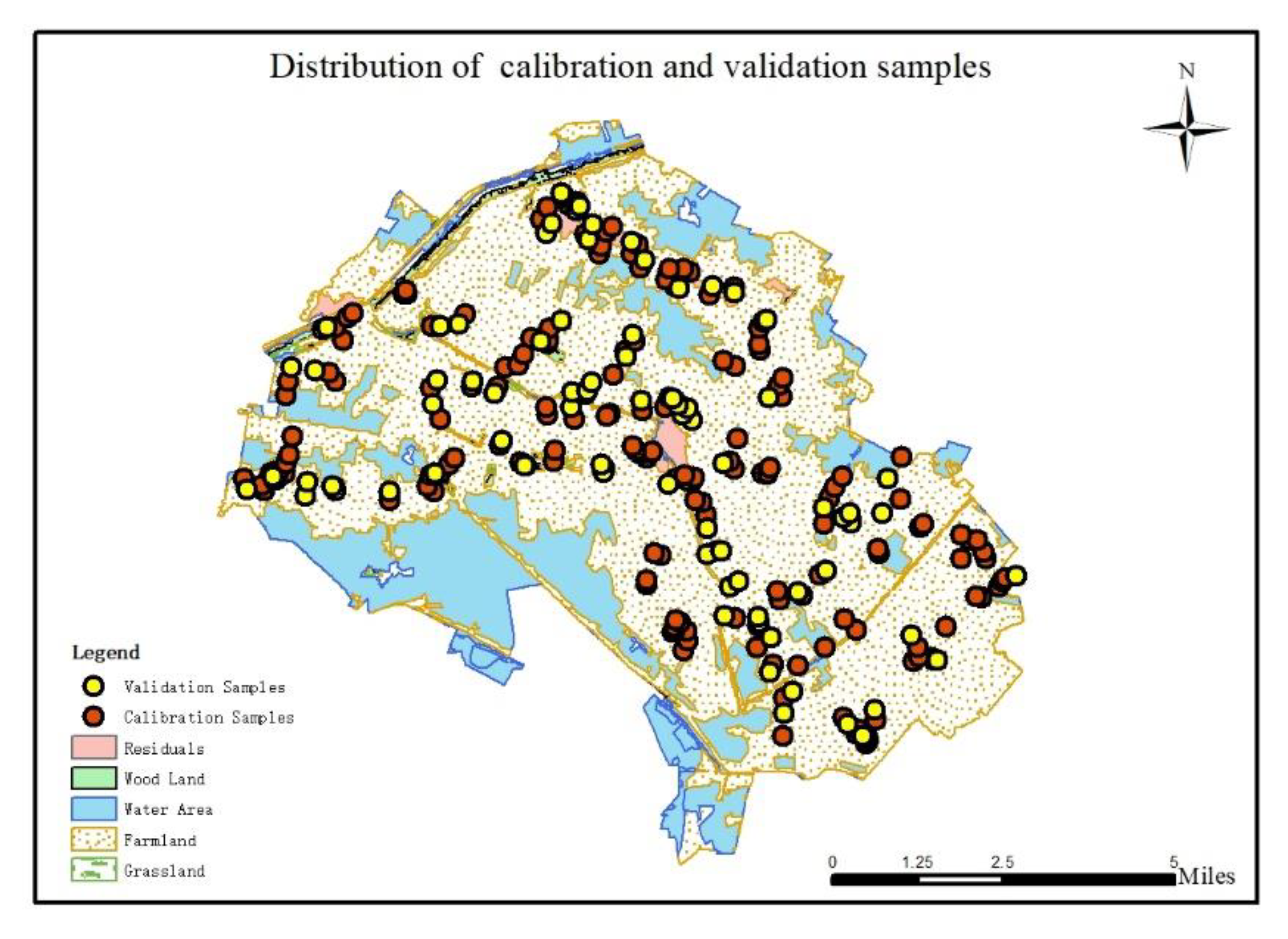
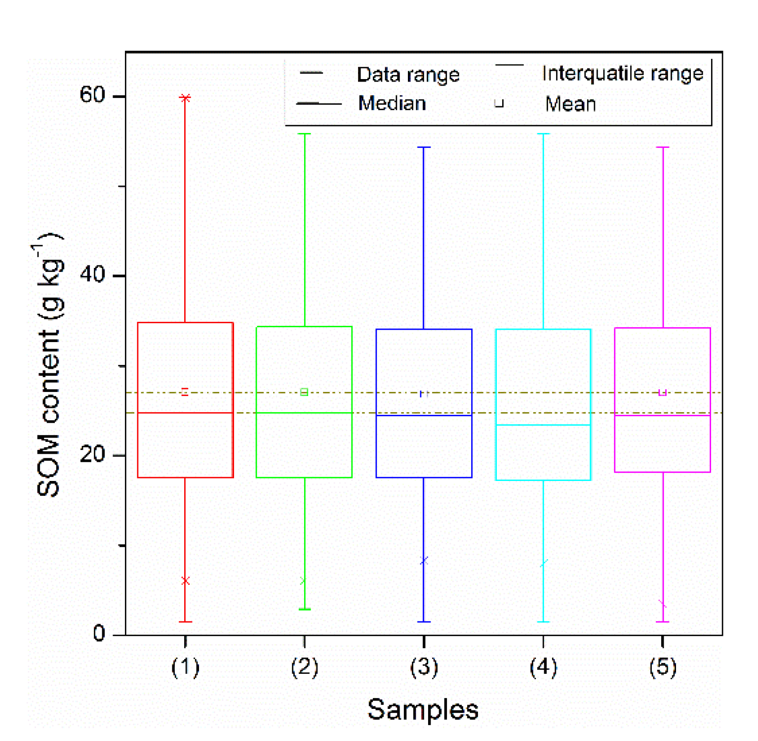
The procedure of selecting the calibration set using the MVARC-R-KS method comprised two phases [3]. Phase 1 consisted of obtaining clustering zones with similar influences of the environment on SOM content. Phase 2 utilized the Rank–KS method to select representative samples from the clustering zones. The selected samples were eventually merged as the calibration set (Figure 4). Typical methods, such as C, KS, and Rank–KS methods, were used for comparison to verify the representation of the calibration set. If the calibration set was representative, then the distribution characteristics of the calibration set would be similar to the entire samples. The statistical values of SOM content and the spectral reflectance information of the calibration sets selected by the aforementioned methods were calculated and are shown in Figure 5 and

Table 3. Statistical values of the spectral reflectance information in the samples.

Statistic Values	All Samples	Samples Selected by Typical Methods
		C	Rank–KS	KS	MVARC-R-KS
Mean	0.3542	0.3495	0.3563	0.3561	0.3541
Variation	0.0369	0.0360	0.0404	0.0401	0.0405

. The results showed that the mean and median values of the SOM content in the calibration set selected by the KS method were lower than those in the entire samples. In contrast to the KS method, the C, Rank–KS, and MVARC-R-KS methods obtained calibration sets having a considerably similar distribution to the entire samples for SOM content. Compared with the calibration sets selected by the KS, Rank–KS, and MVARC-R-KS methods, the calibration set selected by the C method had less similar spectral reflectance information to that of the entire samples. Compared with the C, KS, and Rank–KS methods, the MVARC-R-KS method further took into consideration the spatial variation and impacts of the environmental variables [3].

In summary, the calibration set selected by the MVARC-R-KS method was the SOM content, spectrum representative, and environment representative [3]. Hence, the MVARC-R-KS method seemed to be reasonable to select a representative calibration set.

4.2.2. Performance of the PLS–MARS Model Calibrated by the Calibration Set Selected Utilizing the MVARC-R-KS Method

The PLS–MARS method was used to build the SOM prediction model based on the VNIR spectra in accordance with the selected calibration set (Figure 4). PCs were first calculated and selected. The count of PCs was set at 10, with the highest precision (i.e., RMSEV) of the constructed regression model (Figure 6) based on the PC selection procedure described in Phase 1 of Section 3.2. Thereafter, the PLS–MARS model was constructed based on the PCs and SOM content. The PLS–MARS model was eventually evaluated.

Table 4. Evaluation results of prediction models calibrated by different calibration set selection methods.

Prediction Model	Selection Method	Corrected Akaike Information Criterion (AICc)	${\mathit{R}}_{\mathit{c}}^2$	RMSEV(g kg−1)	${\mathit{R}}_{\mathit{p}}^2$	RMSEP(g kg−1)	RPD
MLR	C	1005.54	0.54	8.9	0.11	28.0	0.44
	KS	973.4	0.62	8.19	0.11	26.0	0.47
	Rank–KS	948.65	0.50	9.04	0.22	23.1	0.52
	MVARC-R-KS	937.79	0.54	8.9	0.09	30.8	0.39
PLS	C	877.64	0.73	6.39	0.53	8.21	1.48
	KS	844.87	0.78	5.87	0.50	8.82	1.38
	Rank–KS	829.80	0.71	6.51	0.56	8.48	1.51
	MVARC-R-KS	785.50	0.79	5.83	0.70	6.98	1.61
SVM	C	996.75	0.54	8.70	0.50	8.78	1.38
	KS	972.02	0.58	8.16	0.39	9.47	1.29
	Rank–KS	912.02	0.55	8.17	0.46	9.34	1.38
	MVARC-R-KS	935.36	0.50	8.84	0.55	8.11	1.56
PLS–GWR	C	1187.90	0.75	5.80	0.54	8.18	1.49
	KS	1227.43	0.79	5.19	0.50	8.76	1.42
	Rank–KS	1190.26	0.76	5.55	0.60	8.02	1.60
	MVARC-R-KS	1213.80	0.74	6.12	0.66	6.83	1.78
PLS–MARS	C	1156.61	0.80	5.45	0.53	8.20	1.48
	KS	1213.20	0.83	5.12	0.55	8.13	1.50
	Rank–KS	1166.12	0.79	5.50	0.62	7.88	1.63
	MVARC-R-KS	1135.50	0.84	5.14	0.71	6.52	1.94

shows the fit assessments of the prediction model. The result indicated that the PLS–MARS model calibrated by the samples selected utilizing the MVARC-R-KS method [3] could estimate SOM content with high stability and prediction precision.

4.2.3. Comparison of the PLS–MARS Model with Typical Prediction Models

The MLR, PLS, SVM, and PLS–GWR methods were utilized to construct the SOM prediction model based on the VNIR spectra in the research region to verify the availability of the PLS–MARS method. The precision of the prediction method was substantially correlated with the selected calibration set. Hence, the C, KS, Rank–KS, and MVARC-R-KS methods were introduced to obtain the representative calibration sets.

The performance of the models was evaluated using fitness assessment indices (e.g., AICc, $R_c^2$, RMSEV, $R_p^2$, RMSEP, and RPD) (Table 4). Two conclusions could be drawn. One was that the performance of the prediction models highly relied on the selected calibration sets; such performance was achieved for the following reasons. The results imply that the accuracies of the models based on different calibration sets fluctuated heavily. For example, the prediction models calibrated using the calibration sets selected by the C and KS methods had poor prediction capabilities. The Rank–KS method selected the calibration set for building prediction models with relatively higher accuracies than those of the C and KS methods. The prediction models calibrated by the samples obtained utilizing the MVARC-R-KS method had the highest prediction accuracies. These results sufficiently verified the dependency of the performance of the prediction models on the selected calibration sets. Because the PLS–GWR model was a local prediction model, the calibration sets had less effect on the prediction results. Another conclusion was that the PLS–MARS method outperformed the typical prediction models for estimating VNIR-spectrum–based SOM content in the study area. The following results support this conclusion. The results in Table 4 show that the MLR model had poor prediction accuracies and thus could not be used to predict SOM content in the study area. The possible reason is due to the inapplicability of these methods for complex high-dimension data sets. Although the PLS and SVM models had relatively higher simulation and prediction accuracies, their model accuracies were lower than the PLS–GWR and PLS–MARS models that considered the local difference. The Moran’s I indexes in Table 1 indicate that both the PLS–MARS model and PLS–GWR model could maintain the spatial heterogeneity distribution characteristics of data. In addition, random spatial residuals without autocorrelation could further verify the effectiveness of the PLS–GWR model and the PLS–MARS model. Compared with the PLS–GWR model, the PLS–MARS model, which considered the nonlinear relationship between SOM content and VNIR spectra, had the highest simulation and prediction accuracies among the prediction models. Since PLS–GWR and PLS–MARS were constructed based on the same PCs, their AICc values were comparable. Nevertheless, the AICc values indicated that the proposed PLS–MARS model had higher model quality than the PLS–GWR model. In summary, the PLS–MARS model calibrated by the samples obtained utilizing the MVARC-R-KS method indicated immense potential for building a prediction model of SOM content based on the VNIR spectra in the riverside region.

5. Discussion

Intrinsic strategies for the prediction method and selected calibration set were significant factors that affected the performance of the constructed prediction model. The influence of the calibration set on model performance, and the good performance of the MVARC-R-KS method and the proposed PLS–MARS prediction method will be discussed in Section 5.1 and Section 5.2, respectively.

5.1. Influence of the Calibration Set on the Model Performance

If the calibration set can well represent the relation of the SOM content with VNIR spectra, then the prediction model calibrated using this calibration set will have a good prediction performance. Table 4 shows that the prediction models calibrated using the calibration sets selected by the classical C and KS methods lacked good prediction performance, whereas the prediction models based on the Rank–KS method could build models with considerably high $R_p^2$ and RPD in the study area. This phenomenon was mainly due to the fact that the calibration set obtained utilizing the C or KS method was representative of either the SOM content or the spectrographic information. By contrast, the calibration set obtained utilizing the Rank–KS method was both SOM content and spectral information representative. These results also indicated that the component concentrations and spectrographic information should be simultaneously taken into account to obtain the representative calibration set to accurately build a VNIR-spectrum–based SOM prediction model. However, in comparison with the Rank–KS method, the MVARC-R-KS method could select the more representative calibration sets, which could calibrate the prediction models with the highest accuracy. This result could be attributed to the consideration of the impact of the surrounding environment and spatial heterogeneity on the samples in the MVARC-R-KS method, which were substantially consistent with real situations.

In summary, the prediction models depended substantially on the selected calibration sets. A representative calibration set instead of a randomly selected calibration set should be obtained in advance to construct a prediction model with good performance. Hence, calibration set selection should be taken seriously during the construction of the prediction models. This study suggests that the MVARC-R-KS method [3] can be set as the optimal choice in the riverside region. This is because this method simultaneously considers the influence of multiple influential factors (i.e., chemical components, spectrographic information, and environmental factors), thereby making the VNIR-spectrum–based SOM prediction model calibrated by the selected calibration set an extensively applicable one.

5.2. Strategies of the PLS–MARS Method

The performance of the PLS–MARS method was analyzed using the simulated data set and real application. In addition, the effectiveness and accuracy of PLS–MARS were compared with those of several commonly used prediction methods (i.e., MLR, PLS, SVM and PLS–GWR methods) in literature. The results in the simulated application implied that the PLS, SVM, and PLS–MARS methods could efficiently estimate the relationship between numerous explanatory variables and their responses. However, if the relationship exhibited significantly non-linear features and spatial heterogeneity, such as the relation of the SOM content with VNIR spectra in the study area, then the PLS–MARS method produced more accurate results than the rest of the prediction methods tested. This superiority is generally due to the consideration of the natural local difference of data sets, and the construction of a local non-linear optimization model in the PLS–MARS method rather than the global non-linear optimization characteristics of the other prediction methods. The adaptive strategy of the PLS–MARS method also facilitated the automatic estimation of natural relationships and supported their promotion. Thus, the PLS–MARS method has immense potential for estimating the complex nonlinear relationships of geographical data with numerous explanatory variables, and the PLS–MARS method calibrated by the samples obtained utilizing the MVARC-R-KS method shows great potential in estimating significantly nonlinear relationships in spatial and non-spatial domains.

6. Conclusions

The PLS–MARS method was proposed to construct a nonlinear model for SOM content prediction, in which the MVARC-R-KS method was adopted to select the optimal calibration set. Several commonly used calibration set selection methods were applied to calibrate the PLS–MARS model, and their influences on the prediction precision of the established model were investigated. The implementation procedure for the proposed method was described in detail. The proposed approach was illustrated and validated through a simulated data set and practical application in the Jianghan Plain. A comparative study with conventional prediction methods indicated that the proposed PLS–MARS method presents the following advantages: (1) the proposed method can efficiently estimate the nonlinear relationship underlying data with numerous variables; (2) the proposed method can accurately construct the highly nonlinear relationship of the SOM content with VNIR spectra, with consideration of the spatial heterogeneity of the relationship; (3) the proposed method can automatically construct a prediction model without substantial prior knowledge of the data set.

The following new findings were obtained based on the application of the PLS–MARS method to estimate SOM content in the Jianghan Plain in China: (1) the accuracy of prediction models, including the PLS–MARS model, depends significantly on the selected calibration sets; (2) the combined PLS–MARS and MVARC-R-KS methods have immense stability and prediction capabilities when estimating the relation of SOM content with VNIR spectra in the study area.

In general, the proposed PLS–MARS method can accurately estimate the nonlinear relationship with local differences. The PLS–MARS method calibrated by the samples obtained utilizing the MVARC-R-KS method has considerable potential for estimating SOM. Furthermore, the PLS–MARS method is conceptually simple and easily executed via a programming language, thereby ensuring easy application.

Future studies will focus on further practical applications of the PLS–MARS method. For example, a PLS–MARS model calibrated by the calibration set selected utilizing MVARC-R-KS method can serve as a potential prediction model to estimate other soil properties (e.g., iron content, copper content, and soil organic C) based on the VNIR spectra in the study area or other areas. The proposed PLS–MARS method can also be used to characterize the nonlinear relationships of other geographic phenomena.

References

1. Singh, M.; Sarkar, B.; Bolan, N.S.; Ok, Y.S.; Churchman, G.J. Decomposition of soil organic matter as affected by clay types, pedogenic oxides and plant residue addition rates. J. Hazard. Mater. 2019, 374, 11–19. [Google Scholar] [CrossRef]
2. Tian, P.; Mason-Jones, K.; Liu, S.; Wang, Q.; Sun, T. Form of nitrogen deposition affects soil organic matter priming by glucose and cellulose. Biol. Fertil. Soils 2019, 55, 383–391. [Google Scholar] [CrossRef]
3. Wang, X.; Chen, Y.; Guo, L.; Liu, L. Construction of the Calibration Set through Multivariate Analysis in Visible and Near-Infrared Prediction Model for Estimating Soil Organic Matter. Remote Sens. 2017, 9, 201. [Google Scholar] [CrossRef] [Green Version]
4. Guo, L.; Zhang, H.; Chen, Y.; Qian, J. Combining Environmental Factors and Lab VNIR Spectral Data to Predict SOM by Geospatial Techniques. Chin. Geogr. Sci. 2019, 29, 258–269. [Google Scholar] [CrossRef] [Green Version]
5. Moura-Bueno, J.M.; Dalmolin, R.S.D.; ten Caten, A.; Dotto, A.C.; Demattê, J.A.M. Stratification of a local VIS-NIR-SWIR spectral library by homogeneity criteria yields more accurate soil organic carbon predictions. Geoderma 2019, 337, 565–581. [Google Scholar] [CrossRef]
6. Liu, Y.; Chen, Y. Estimation of total iron content in floodplain soils using VNIR spectroscopy—A case study in the Le’an River floodplain, China. Int. J. Remote Sens. 2012, 33, 5954–5972. [Google Scholar] [CrossRef]
7. Liu, Y.; Chen, Y. Feasibility of Estimating Cu Contamination in Floodplain Soils using VNIR Spectroscopy—A Case Study in the Le’an River Floodplain, China. Soil Sedim. Contam. An Int. J. 2012, 21, 951–969. [Google Scholar] [CrossRef]
8. Liu, Y.; Guo, L.; Jiang, Q.; Zhang, H.; Chen, Y. Comparing geospatial techniques to predict SOC stocks. Soil Tillage Res. 2015, 148, 46–58. [Google Scholar] [CrossRef]
9. Liu, Y.; Song, Y.; Guo, L.; Chen, Y.; Lu, Y.; Liu, Y. Geostatistical models of soil organic carbon density prediction based on soil hyperspectral reflectance. Trans. Chin. Soc. Agric. Eng. 2017, 33, 183–191. [Google Scholar]
10. Tekin, Y.; Tümsavas, Z.; Mouazen, A.M. Comparing the artificial neural network with parcial least squares for prediction of soil organic carbon and pH at different moisture content levels using visible and near-infrared spectroscopy. Rev. Bras. Ciência Solo 2014, 38, 1794–1804. [Google Scholar] [CrossRef] [Green Version]
11. Liess, M.; Schmidt, J.; Glaser, B. Improving the Spatial Prediction of Soil Organic Carbon Stocks in a Complex Tropical Mountain Landscape by Methodological Specifications in Machine Learning Approaches. PLoS ONE 2016, 11, e0153673. [Google Scholar]
12. Huang, N.; Wang, L.; Guo, Y.; Niu, Z. Upscaling plot-scale soil respiration in winter wheat and summer maize rotation croplands in Julu County, North China. Int. J. Appl. Earth Obs. Geoinf. 2017, 54, 169–178. [Google Scholar] [CrossRef]
13. Laamrani, A.; Berg, A.A.; Voroney, P.; Feilhauer, H.; Blackburn, L.; March, M.; Dao, P.D.; He, Y.; Martin, R.C. Ensemble Identification of Spectral Bands Related to Soil Organic Carbon Levels over an Agricultural Field in Southern Ontario, Canada. Remote Sens. 2019, 11, 1298. [Google Scholar]
14. Zheng, G.; Zhang, W.B.; Zhou, H.Z.; Yang, P.B. Multivariate adaptive regression splines model for prediction of the liquefaction-induced settlement of shallow foundations. Soil Dyn. Earthq. Eng. 2020, 132, 10. [Google Scholar]
15. Huang, H.; Ji, X.L.; Xia, F.; Huang, S.H.; Shang, X.; Chen, H.; Zhang, M.H.; Dahlgren, R.A.; Mei, K. Multivariate adaptive regression splines for estimating riverine constituent concentrations. Hydrol. Process. 2020, 34, 15. [Google Scholar] [CrossRef] [Green Version]
16. Liu, L.-L.; Cheng, Y.-M. Efficient system reliability analysis of soil slopes using multivariate adaptive regression splines-based Monte Carlo simulation. Comput. Geotech. 2016, 79, 41–54. [Google Scholar] [CrossRef]
17. Brillante, L.; Bois, B.; Mathieu, O.; Lévêque, J. Electrical imaging of soil water availability to grapevine: A benchmark experiment of several machine-learning techniques. Precis. Agric. 2016, 17, 637–658. [Google Scholar] [CrossRef]
18. Guo, L.; Zhao, C.; Zhang, H.; Chen, Y.; Linderman, M.; Zhang, Q.; Liu, Y. Comparisons of spatial and non-spatial models for predicting soil carbon content based on visible and near-infrared spectral technology. Geoderma 2017, 285, 280–292. [Google Scholar] [CrossRef]
19. De Jong, E.; Schappert, H.J.V. Calculation of soil respiration and activity from CO2 profiles in the soil. Soil Sci. 1972, 113, 328–333. [Google Scholar]
20. Tang, J.; Baldocchi, D.D.; Qi, Y.; Xu, L. Assessing soil CO2 efflux using continuous measurements of CO2 profiles in soils with small solid-state sensors. Agric. Forest Meteorol. 2003, 118, 207–220. [Google Scholar]
21. Technometrics. Index to contents, Volume 11, 1969. Technometrics 1969, 11, 848–851. [Google Scholar] [CrossRef]
22. Liu, W.; Zhao, Z.; Yuan, H.; Song, C.; Li, X. An optimal selection method of samples of calibration set and validation set for spectral multivariate analysis. Spectrosc. Spectr. Anal. 2014, 34, 947–951. [Google Scholar]
23. Liu, Y.; Lu, Y.; Guo, L.; Xiao, F.; Chen, Y. Construction of Calibration Set Based on the Land Use Types in Visible and Near-InfRared (VIS-NIR) Model for Soil Organic Matter Estimation. Acta Pedol. Sin. 2016, 53, 332–341. [Google Scholar]
24. Rana, P.; Gautam, B.; Tokola, T. Optimizing the number of training areas for modeling above-ground biomass with ALS and multispectral remote sensing in subtropical Nepal. Int. J. Appl. Earth Obs. Geoinf. 2016, 49, 52–62. [Google Scholar] [CrossRef]
25. Friedman, J.H.; Roosen, C.B. An introduction to multivariate adaptive regression splines. Stat. Methods Med. Res. 1995, 4, 197–217. [Google Scholar] [CrossRef] [PubMed]
26. Brunsdon, C.; Fotheringham, S.; Charlton, M. Geographically Weighted Regression. J. R. Statal Soc. Ser. D (Statian) 1998, 47, 431–443. [Google Scholar] [CrossRef]
27. Hurvich, C.M.; Simonoff, J.S.; Tsai, C.L. Smoothing parameter selection in nonparametric regression using an improved Akaike information criterion. J. R. Statal Soc. 1998, 60, 271–293. [Google Scholar] [CrossRef]
28. Shi, T.; Cui, L.; Wang, J.; Fei, T.; Chen, Y.; Wu, G. Comparison of multivariate methods for estimating soil total nitrogen with visible/near-infrared spectroscopy. Plant Soil 2012, 366, 363–375. [Google Scholar] [CrossRef]
29. Viscarra Rossel, R.A.; McGlynn, R.N.; McBratney, A.B. Determining the composition of mineral-organic mixes using UV–vis–NIR diffuse reflectance spectroscopy. Geoderma 2006, 137, 70–82. [Google Scholar]
30. Chen, Y. Spatial Autocorrelation Approaches to Testing Residuals from Least Squares Regression. PLoS ONE 2016, 11, e0146865. [Google Scholar] [CrossRef] [Green Version]
Figure 1. Distribution of the soil samples.
Applsci 11 00566 g001
Figure 2. (a) Pretreatment spectral curves of the soil samples. (b) Continuum removed spectral curves of the soil samples.
Applsci 11 00566 g002
Figure 3. Procedure of constructing the partial least squares–based multivariate adaptive regression spline (PLS–MARS) model.
Applsci 11 00566 g003
Figure 4. Calibration and validation samples selected utilizing the regional multi-variable associate rule mining and Rank–Kennard-Stone (MVARC-R-KS) method.
Applsci 11 00566 g004
Figure 5. Statistics of the soil organic matter (SOM) content in the following samples: (1) all samples; (2) samples selected utilizing the concentration gradient (C) method; (3) samples selected utilizing the Rank–Kennard-Stone (Rank–KS) method; (4) samples selected using the Rank method; (5) samples selected utilizing the MVARC-R-KS method.
Applsci 11 00566 g005
Figure 6. Root-mean-square error (RMSEV) of the prediction model constructed using the latent variables (i.e., principal components (PCs)).
Applsci 11 00566 g006