Abstract
The paper presents a multiaspect analysis of multivalues and the broadband nature of system oscillation. By analyzing the ambient signal caused by random small disturbances during the normal operation of interconnected power grids, many system operation characteristics can be obtained. The traditional signal processing method cannot extract the information from ambient signals effectively. Aiming at the problem of broadband oscillation mode superposition and the difficulty of extracting information from ambient signals, an iterative adaptive variational mode decomposition (IA-VMD) method is proposed based on frequency domain analysis and signal energy. Additionally, the IA-VMD method, combined with a bandpass filter and the Prony algorithm, is used to realize the modal identification of broadband oscillation and ambient signals. Simulation experiments show that the IA-VMD method has good adaptability, antinoise characteristics, and a certain significant engineering application value as well.
1. Introduction
In recent years, with the development of electric power technology and the scale of power grids, power exchanges across regions and over long distances have become more common. However, this outcome brings many new security problems to power grids, among which the low-frequency oscillation (LFO) of the power system is a very important problem [1,2]. If the power grid oscillation is not detected and suppressed in time, it may have a serious impact on the power system.
At present, the analysis methods for LFOs of power systems mainly include offline analysis methods based on mathematical models of power systems [3,4] and signal analysis methods based on measured signals. The former method has problems such as the uncertainty of the operation mode of the power grid and the curse of dimensionality in the calculation process; these problems make it difficult to apply this method to the online monitoring of LFOs. Compared with the former method, the latter method can better adapt to the operation mode of the power grid. The acquisition of measured signals is not restricted by the size of the power system, which can reduce the difficulty of oscillation analyses. Additionally, by identifying and analyzing the system output signal, the system characteristics contained in the signal can be obtained. In recent years, a wide area measurement system (WAMS) has been widely applied to power systems, which provides the foundation for signal analysis methods. Therefore, the signal analysis method, based on measured signals, has become the main analysis method of power system LFOs [5].
There are many small fluctuation signals, called ambient signals (similar to environmental noise), in the normal operation of the power grid [6]. Ambient signals are generally caused by normal electrical operation during the operation of a power grid, such as load switching and line parameter adjustment. These signals widely exist in measurement signals, contain rich characteristic information of system operation, and can be used for early warning of oscillation. However, ambient signals are easily obscured by environmental noise, so how to extract the characteristic information of system operation from these signals is a key problem [7].
At present, there are many methods used to analyze LFO, such as discrete Fourier transform (DFT) [8], empirical mode decomposition (EMD) [9], wavelet-based methods [10], Hilbert–Huang transform (HHT) [11], estimation of signal parameters via rotational invariance technique (ESPRIT) [12,13,14], matrix pencil [15] and the Prony algorithm [16].
In [13], a method combining ESPRIT with the exact model order (EMO) was proposed to analyze LFO. In addition, in [15], the basis pursuit denoising method, combined with a tuneable Q-factor wavelet transform, was proposed to increase the signal-to-noise ratio, and then an improved version of the matrix pencil algorithm was used to identify the parameters of LFO.
The Prony algorithm, the most widely used method in many oscillation mode parameter extraction algorithms, can fit the actual LFO signals by a linear combination of multiorder exponential functions. The oscillation characteristic parameters of the oscillation signal can be obtained directly by using the Prony algorithm. However, the Prony algorithm is sensitive to noise, so it cannot identify the ambient noise signals of the power grid directly [17,18]. Therefore, it is necessary to perform modal decomposition on the measured signals so as to obtain modal parameters by the Prony algorithm in the future.
At present, there are multiple modal decomposition methods, such as the Kalman filter, wavelet transform, EMD, eigensystem realization algorithm (ERA), and variational mode decomposition (VMD). By combining the above methods with the Prony algorithm, the interference in the original signal can be removed and the identification accuracy of the Prony algorithm can be greatly improved [19,20,21]. Among the above methods, the scheme of the VMD method, combined with the Prony algorithm, can obtain relatively high identification accuracy.
The VMD method can be used to decompose ambient noise signals into finite intrinsic mode functions (IMFs). Then, the potential oscillation modal information can be obtained by using the Prony algorithm. In this paper, a scheme of bandpass filtering, combined with the IA-VMD algorithm and the Prony algorithm, is proposed. The experimental results show that IA-VMD combined with the Prony algorithm has improved accuracy.
The performance of the IA-VMD method for power system oscillation identification is studied in this paper. The model of ambient signals and the framework of VMD-based LFO identification are given in Section 2. The IA-VMD mode identification method and the Prony algorithm are introduced in Section 3 and Section 4, respectively, and the performance of the method for analyzing LFO in a power system is studied in Section 5. Section 6 provides conclusions.
2. Framework of VMD-Based LFO Identification
2.1. Broadband Ambient Model
Broadband oscillatory signals are constructed as follows. The original broadband signal S0(t) contains several oscillatory modal signals of different frequency bands, ambient signals of system operating parameters, and noise signals in the process of measurement and transmission. The original measurement signal S0(t) is expressed as
In the formula, S0(t) represents the measured signal collected by the system, Si(t) (i = 1,2,..., N) represents the oscillation signal in the i-th frequency band, R(t) represents the residual modal component containing the trend component, and N0(t) represents the persistent environmental noise and transmission noise in the system. The oscillation morphology of oscillation modal signal Si(t) in each frequency band is decomposed as follows:
In the formula, Si(t) represents oscillation signals of different frequency bands, and each frequency band oscillation signal consists of multiple inherent modes. IMFk (t) (k = 1,2,..., N) represents the k-th different inherent oscillation mode signal and its expression is shown as follows:
In the formula, Uk(t) represents the amplitude of the k-th intrinsic modal component varying with time, fk represents the frequency of the k-th intrinsic modal component, and Dk represents the damping ratio of the k-th intrinsic modal component.
2.2. The Framework of the VMD Method
The framework of VMD-based oscillation identification from ambient signals is shown in Figure 1. S0(t) represents the ambient signal generated by the normal electrical operation during the operation of the power grid. K represents the number of IMFs contained in the ambient signal. First, the measured ambient signal must be preprocessed and detrended. Then, the value of K can be obtained by the improvement of the VMD method, and each IMF can be decomposed using the VMD method. Finally, the oscillation characteristics of the main modes, such as frequency, amplitude, and damping ratio, can be extracted by using the Prony algorithm.
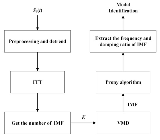
Figure 1.
Framework of variational mode decomposition (VMD)-based oscillation identification from an ambient signal.
The variational mode decomposition algorithm is a new adaptive signal decomposition method first proposed by Dragomiretskiy et al. in 2014 [22]. In the process of mode decomposition, the VMD algorithm uses a cyclic iteration method to obtain the optimal solution of the constrained variational problem, and then the intrinsic mode component and its frequency center and bandwidth can be obtained. Finally, the intrinsic mode component of the original signal is separated.
VMD retains some of the advantages of EMD; there is no need to set the decomposition basis or to adjust the stationarity assumption. On this basis, a new approach is proposed to solve the mode aliasing problem, which easily appears when the EMD algorithm is used to decompose approximate frequency modes. Different from the classical EMD method, the new EMD method defines the IMF component mode as a signal in which the number of poles and zeros is less than 1 and VMD defines the IMF component as an AM–FM signal. Obviously, the definition of the VMD algorithm is relatively rigorous.
2.3. Ambient Data Selection
The WAMS signal can be classified into obvious oscillation signals and ambient signals. Ambient signals are raised by small disturbances, such as load changes in normal operation. This information is easy to collect and can be obtained directly in WAMS.
2.4. Processing and Detrending
DC offset and trend components affect the estimation results, so we need to remove the trend component by linear fitting. If some data are lost, we can use linear interpolation to solve this problem; this processing method does not affect the accuracy of the analysis results.
3. The Iterative Adaptation VMD Method
In fact, the VMD method extends the classical Wiener filter to multiple adaptive wavebands. Compared with EMD and local mean decomposition (LMD), the VMD method has the advantages of fast convergence, high robustness, and better performance in antinoise regulation and nonstationary signal processing.
As shown in Figure 2, the bandpass filter (BPF) method preliminarily decomposes the original input signal according to the frequency range of the LFO interval mode, the LFO local mode, subsynchronous oscillation (SSO), and supersynchronous oscillation (SurSO). The intrinsic mode function of each frequency band signal can be obtained by the IA-VMD method. Finally, the frequency, damping ratio, and oscillation amplitude of each IMF can be extracted by the Prony algorithm.
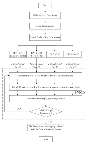
Figure 2.
Framework of iterative adaptive variational mode decomposition (IA-VMD)-based broadband oscillation identifications.
3.1. Intrinsic Mode Function
The signal S(t) can be decomposed into several intrinsic mode functions with center frequency and limited bandwidth using the VMD method. Intrinsic mode functions are amplitude-modulated–frequency-modulated signals, written as (see [23])
where the envelope is non-negative Ak(t), is the instantaneous frequency of uk(t), uk(t) is a set of discrete subsignals, and the bandwidth sparsity of each subsignal is different in the spectral domain [22].
Each modal component is close to the center frequency ωk. The bandwidth is estimated through the H1 Gaussian smoothness of the demodulated signal. Due to the sparsity of VMD, the resulting constrained variational problem is the following:
where {uk}: = {u1, …, uk} represents the K components of signal S(t), and {ωk}: = {ω1, …, ωk} represents the center frequencies of each component; represents a partial derivative of t; is convolution operation; is the unit impulse function; S(t) is the signal obtained after the original signal is filtered by bandpass filter.
3.2. Alternate Direction Method of Multipliers
To obtain the optimal solution of the above constrained variational problem, the Lagrangian multipliers λ and quadratic penalty α are used to render the problem of (3) unconstrained, as follows:
By using the alternate direction method of multipliers (ADMMs) to find the saddle point of Lagrangian L, the optimal solution of the original minimization problem can be obtained. The implementation process of ADMM optimization for VMD is as follows:
(1) Initialize, k = 0, n = 0, where ,, and are the Fourier transforms of , x(t), and λn, respectively. K is the number of components, and n is the number of iterations.
(2) n = n + 1; start the iteration cycle;
(3) k = k + 1, according to the following formula update uk, until k = K:
(4) Update ωk:
(5) Update λk:
(6) Set the evaluation precision ε > 0. When ε satisfies , end the loop and output IMF components; otherwise, repeat steps (3)–(6).
3.3. The Estimation of Mode Number K
Compared to the EMD algorithm, the VMD algorithm not only retains the advantages of the EMD algorithm but also offers better fitting accuracy, improved decomposition results, and a faster running speed. However, the traditional VMD method has its own disadvantages. On the one hand, the preset value of K is mainly set according to operational experience. This parameter affects the accuracy of the oscillation decomposition of the VMD algorithm. However, modal confusion may occur in the case of high-noise signals. The traditional VMD method can only distinguish the ambient signal from the environmental noise and cannot extract the IMF directly.
To make the VMD algorithm better adapted to ambient signals, this paper improves the VMD algorithm in two aspects. On the one hand, to increase the accuracy of the decomposition results, the self-adaptability of the algorithm is improved to choose a suitable value of K; on the other hand, the signal energy method is introduced to screen the intrinsic modal components obtained from the first decomposition so as to further reduce the influence of high-noise signals. This paper combines the VMD algorithm with frequency domain analysis by introducing a frequency domain analysis method. The steps for estimating the number of modal components K are as follows:
Step 1: Obtain the frequency diagram of the measured signal by fast Fourier transform (FFT).
Step 2: Take the data of 0.2 Hz~2 Hz in the spectrum and calculate the average magnitude of the signal in this frequency band.
Step 3: Extract data segments where the magnitude is higher than 3 times the average magnitude. When there is no oscillation, the signal will only contain direct current components and noise components. So, there will be many low amplitude peaks in the spectrum that do not correspond to oscillations. By this step, the influence of noise and interference in the nonoscillation period can be effectively removed.
Step 4: Count the peak number of each extracted data segment by evaluating whether the data are monotonically increasing. The sum of the peak numbers of all the extracted data segments is the mode number K.
Step 5: If the LFO characteristic of the modes is not obvious, decompose the mode by the VMD method again; then, extract the dominant mode.
Aiming at the iterative improvement of the traditional VMD method, this paper introduces the signal energy method to screen the oscillation modes obtained by the first mode decomposition and then improves the VMD algorithm’s decomposition process as follows:
(1) The signal energy Eimf (i) of each modal component is calculated according to Parseval’s theorem. The formulas are as follows:
In the formula, i represents the number of intrinsic modal components, j represents the discrete sampling points of the signal, fi,j(tj) represents the sampling signal, xi,j represents the discrete sampling points of the signal, and Eimf (i) is the signal energy of the ith intrinsic modal component. IA-VMD of the sampled signal can obtain i inherent modal components, in which the modal component with higher signal energy is called the dominant modal component. This component can reflect the operation characteristics of the system. The specific steps of extracting dominant modal components are as follows:
(2) The signal energy value Eimf (i) of each intrinsic modal component can be calculated by Formula (10). The sum of the signal energy values of each modal component is the total energy value EIMF of the sampled signal oscillation signal. The formula for calculating the total energy value of the oscillation signal is as follows:
(3) In [24], it can be found that the oscillation characteristic parameters of modal components with a high proportion of energy can provide a reference for the analysis of the sampling signal characteristics. When the calculated modal energy weight is larger than the threshold value ε, the modal component is extracted and set as the main oscillating mode. Otherwise, this component is ignored. The formula for calculating the energy weight of the component signal is as follows:
(4) The intrinsic modal components with higher signal energy are screened out by the signal energy method, and the intrinsic modal component value K is updated. Additionally, the intrinsic modal components finally obtained correspond to the main operating modes of the system. The operating characteristic parameters of the system can be obtained by parameter identification of the dominant intrinsic modal components.
The modal component with higher signal energy has a higher oscillation amplitude and weaker damping. The power of these modal components varies greatly and is easy to diverge, which poses a great threat to the safe and stable operation of power systems. The decomposition and research of dominant inherent modal components is the key to power system stability analysis.
If the frequencies of the two dominant modal components are close, traditional VMD may lead to the problem of mode aliasing. By using IA-VMD of the dominant modal components, the problem of mode aliasing can be solved eventually, and the dominant modal components with clearer oscillation mode decomposition can be more easily identified in the next step.
4. Prony Algorithm
The Prony algorithm aims to estimate the parameters for the exponential terms through the following fitting function:
where is the sampled signal of , and Δt is the sample interval. Additionally, is the Prony fitting function, which is the approximate value of the sampled signal x(n). N is the number of sampling points of signals to be analyzed, as acquired by the system. In general, suppose that bi, zi is a complex number and represents attenuation characteristics and oscillation characteristics of the sampled signal, respectively.
where Ai, θi, fi, and αi are the amplitude, damping factors, frequency, and phase associated with the ith mode, respectively.
(1) The first step of the Prony algorithm is to construct a data matrix:
where r(i,j) is the sampled data, and pe is the order of the linear prediction model. The Prony algorithm uses the minimum error sum of squares as the estimation principle of model parameters.
The sample function matrix R of the expansion order is constructed as follows:
where p is the effective order of matrix R. In general, pe is larger than p, but the operation speed will be affected if pe is too large. So, pe can be taken as an integer less than N/2 in actual calculations.
(2) Using the singular value decomposition and total least squares (SVD-TLS) method, obtain the effective order p of the sample function matrix R.
(3) Establish the linear matrix equation to solve the parameter {a0, …, ap}, as follows:
(4) Obtain the characteristic root z by solving the polynomial equation, as follows:
(5) Establish the linear matrix equation to solve the parameter {b0, …, bp}, as follows:
where , the matrix Z is a Vandermonde matrix with a dimension of N×P; it is a full-rank matrix. Additionally, the least-squares solution of Formula (20) can be obtained as follows:
(6) Finally, by Formula (21), the characteristic parameters of the ith oscillation mode, including amplitude, phase, frequency, and damping ratio, can be obtained as the following formulas:
5. Simulation
Firstly, the IA-VMD method is used to identify the constituent broadband oscillation signal. It has been verified that the IA-VMD method has better identification accuracy than other methods for broadband oscillation. Then, the actual LFO events in the Hunan power grid in June 2018 are used to further verify the effect of the IA-VMD method. Before the LFO divergence, the phasor measurement unit (PMU) captured a small amplitude of power fluctuation, which is the measured ambient signal. Because the amplitude of the signal fluctuation was too small, the PMU did not provide a warning. Through the study of this LFO event, this paper proves that the measured ambient signal can be analyzed and it can provide a reference for the early warning of LFOs in the system.
5.1. Analysis of the Test Signal
As described in Section 2 on the broadband ambient noise model, the simulation signal St is constructed to test the effectiveness of the proposed method. St is constructed by the formula, as follows:
The test signal St is composed of broadband signals. The order of dominant frequencies is the LFO interval mode SLFO1, LFO local mode SLFO2, subsynchronous oscillation SSSO1, and supersynchronous oscillation signal SSurSO. Additionally, SSurSO is accompanied by SSSO1; that is, the sum of the frequencies is 120 Hz. SSSO2 is another independent subsynchronous oscillation signal, and SN represents environmental noise.
To make the simulation result closer to the actual situation, the test signal is constructed according to the following requirements:
- (1)
- The test signal should include the signals of each frequency band, and the frequency of each oscillation signal should be selected randomly in its frequency band;
- (2)
- The oscillation amplitude should be selected according to the actual operation situation, and the oscillation amplitude of each frequency band decreases, in turn, from low to high;
- (3)
- Supersynchronous oscillation is accompanied by subsynchronous oscillation. The amplitude of supersynchronous oscillation should be slightly lower than that of subsynchronous oscillation. To satisfy the above conditions, the test signals are selected as follows:
Test signal St is composed of five oscillating signals with different frequencies and white noise with an amplitude of 0.2. Test signal St ranges from 0.5 to 100 Hz. The test signal is shown in Figure 3.
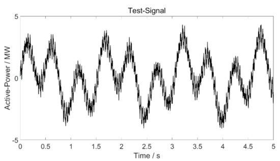
Figure 3.
Test signal.
According to the broadband signal identification process proposed in this paper, test signal St is decomposed into several modes by bandpass filtering and the IA-VMD method, and the dominant oscillation modes of the test signal in different frequency bands are obtained. All oscillation modes of each frequency band of the test signal decomposed by the IA-VMD method are shown in Figure 4. Figure 4 shows that the method proposed in this paper can effectively decompose and extract the oscillation modes in different frequency bands from the test signal.
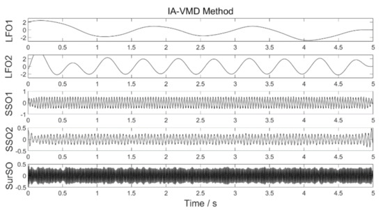
Figure 4.
All modes of the signal with noise after IA-VMD.
After the oscillation modes of each frequency band are obtained, the information of the modal characteristic parameter can be extracted using the Prony algorithm.
The identification results of the proposed method in this paper and the traditional method were compared, and the fitting errors of the different methods are shown in Table 1.

Table 1.
Fitting errors of the different methods.
Compared with the identification results in Table 1, when the test signal is composed of broadband signals, the IA-VMD method combined with the Prony algorithm has the best decomposition and fitting effect among the three methods. Table 1 shows that the maximum fitting error of the oscillation frequency is 1.55%, and the average fitting error is only 0.67%. Thus, the fitting degree of oscillation frequency is good, confirming that the proposed method can meet the requirements of oscillation frequency identification. Table 1 shows that the maximum error of the oscillation amplitude is 9.09%, and the average error is 2.54%. Because the amplitude of subsynchronous oscillation itself is small, the deviation of amplitude identification is large, but it is still in existence. The simulation results show that the proposed method has improved effectiveness in broadband oscillation identification.
Table 1 shows that the EMD–Prony method can accurately identify the two modes of LFO; the fitting errors of the oscillation frequencies are 0 and 1.04%. However, this method has a poor identification effect on subsynchronous oscillations; the fitting errors of the oscillation frequencies are 22.45% and 13.64%. In addition, supersynchronous oscillation cannot be identified by this method. The EMD–Prony method is obviously less effective. Table 1 shows that the MF–Prony method has a very poor identification effect. The maximum fitting error of the oscillation amplitude is 17.81%, which is higher than that of other identification methods. This method cannot even identify subsynchronous oscillation and supersynchronous oscillation. Especially when the test signal contains high-frequency and low-amplitude modes, the traditional Prony algorithm is very sensitive to noise. Therefore, in general, the signal cannot be directly identified by the Prony algorithm.
5.2. Analysis of the Measured Signal
To prove the effectiveness of the method proposed in this paper, the actual oscillation data of a real power grid are selected, and the method is used to identify and analyze the oscillation modes of the measured signal.
The actual oscillation signal collected from the real power grid is shown in Figure 5. When the system runs to 130 s, an obvious oscillation signal appears. After 20 s, the oscillation diverges rapidly, and the power grid alarms at the same time. After 170 s, the oscillation begins to attenuate, later returning to normal. Before the obvious oscillation of the system occurs, there is a small amplitude fluctuation in the system between 70 and 120 s. However, at this time, the system considers that the ambient data are generated by the normal electrical operation of the power grid and does not give an alarm, and the system has a significant disturbance approximately 20 s after the noise-like attenuation. The data interval between the ambient signal and the obvious oscillation signal is shown in Figure 5. Considering the possibility of broadband oscillation, the sampling frequency of the signal is 100 Hz in this paper.
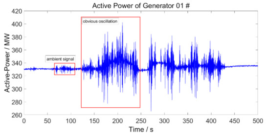
Figure 5.
The actual oscillation signal collected.
The data can be classified into normal data and abnormal data. Ambient signals are a type of normal data, while oscillation signals are a type of abnormal data. The ambient signals of 65–110 s and the obvious oscillation signals of 165–210 s are selected as the research objects, and the operation characteristic modes are identified by the method proposed in this paper. The obvious oscillation signal is shown in Figure 6, and the ambient signal is shown in Figure 7.
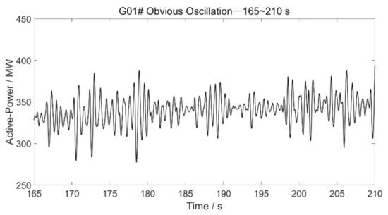
Figure 6.
Obvious oscillation signal collected.
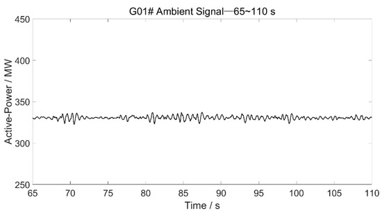
Figure 7.
Ambient noise signal collected.
Figure 7 shows that the oscillation amplitude is small and the amplitude fluctuation is less than 10 MW. In addition, the signal-to-noise ratio (SNR) of this signal is low, so the signal is easily affected by environmental noise, and it is more difficult to identify the oscillation information from the ambient noise signal. We find that the characteristic of the ambient signal is not obvious. Observing Figure 6, we find that the oscillation signal has an obvious oscillation mode, and the oscillation amplitude is higher; the maximum value is over 100 MW, not less than 30% of the active power of the system. The signal has a high SNR, is less affected by environmental noise, and is easy to identify.
The IA-VMD method is used to address the obvious oscillation signal, and the oscillation mode signals in each frequency band after the first decomposition are shown in Figure 8. Then, IMF4 is ignored by the signal energy method. So, three main oscillation modes are obtained from the obvious oscillation signal by the IA-VMD method. The parameters of the main oscillation modes are identified, and the LFO parameters are obtained, as shown in Table 2.
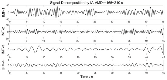
Figure 8.
Intrinsic mode functions (IMFs) extracted from the obvious oscillation signal.
Table 2.
Modal identification of the obvious oscillation signal.
The main oscillation modes decomposed by the IA-VMD method were identified by the Prony algorithm and compared with the MF-Prony method and the EMD-Prony method. The results are shown in Table 2. Table 2 shows that when there are obvious oscillation signals in the processing system, the above three methods can identify a variety of oscillation modes. Relatively speaking, the identification results of this method are close to those of the EMD-Prony algorithm. It can be concluded that the oscillation caused by this accident consists mainly of two obvious oscillation modes. The dominant oscillation frequency is approximately 1.48 Hz, and the secondary dominant oscillation frequency is approximately 2 Hz. Compared with the two algorithms above, the MF-Prony algorithm has a certain deviation in identification results.
Similarly, the method proposed in this paper was used to address the ambient noise signal shown in Figure 7; the main mode signals extracted from the ambient signal by the first decomposition are shown in Figure 9. The signal energy method was used to screen the modes, and all the oscillation modes were retained finally. The decomposed signals were sorted into four dominant modes with decreasing amplitudes.
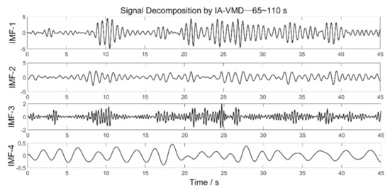
Figure 9.
IMFs extracted from the ambient signal.
The modal parameters of each dominant mode were identified using the three methods; the results are shown in Table 3. As shown in Table 3, the frequencies of the dominant oscillation modes are 1.47, 1.78, 3.59, and 0.32 Hz, with decreasing amplitude. Compared with the results in Table 2, the frequencies of the potential dominant modes extracted from the ambient noise signal are close to those of the dominant modes in the obvious oscillation signals, which are both near 1.48 Hz. As shown in Table 3, the dominant frequency of the EMD–Prony method is 1.55 Hz, and the dominant frequency of the MF–Prony method is 3.74 Hz. There are some deviations between the identification results of the EMD–Prony method and the IA-VMD–Prony method. In comparison, the deviation between the identification results of the MF–Prony method and the IA-VMD–Prony method is very large.
Table 3.
Modal identification of the ambient signal.
On the one hand, the experimental results show that the ambient noise signal contains some of the oscillation characteristics of potential LFOs. On the other hand, the results prove that the method proposed in this paper is suitable not only for analyzing obvious oscillation signals but also for analyzing ambient signals in normal operation; it has high accuracy. Relatively speaking, all the identification results of the other two classical identification methods have large errors. The experimental results show that the method proposed in this paper has a superior result when analyzing ambient signals.
6. Conclusions
In this paper, a new method based on the IA-VMD method and a bandpass filter is proposed to identify broadband oscillation signals. This method can solve problems (including mode aliasing and noise effect) that cannot be solved by the traditional signal identification method, and it also meets the requirements of modal identification. This method can identify the LFO interval mode, the LFO local mode, subsynchronous oscillation, and supersynchronous oscillation from broadband signals. In addition, this method can identify not only the modes of obvious oscillation signals after a disturbance but also ambient signals before the disturbance. It can also identify the oscillation characteristic parameters of potential oscillation from ambient signals, and the parameters provide a reference for the early warning of oscillations of the power system.
In this paper, the proposed method was used to identify obvious oscillation signals after a disturbance and ambient signals before the disturbance, and the results were compared. By comparing the identification results of the two types of signals, it was found that the two frequencies were very close to each other. Therefore, it is further verified that the new method proposed in this paper has good application in mode identification and early warning of system oscillation.
Author Contributions
Methodology, F.L.; Supervision, K.L. and D.S.; Validation, R.Z.; Writing—original draft, S.L.; Writing—review & editing, C.C. All authors have read and agreed to the published version of the manuscript.
Funding
This research was supported by the National Natural Science Foundation of China under Grant 61973318, the Distinguished Young Foundation of Hunan Province of China under Grant 2020JJ2045, the Key R&D Program of Hunan Province of China under Project 2020WK2007, and the Fundamental Research Funds for the Central Universities of Central South University 1053320190264. Denis Sidorov was supported by the base part of the Government Assignment for Scientific Research from the Ministry of Science and Higher Education of Russia, project code: FZZS-2020-0039.
Informed Consent Statement
Not applicable.
Data Availability Statement
The data presented in this study are available on request from the corresponding author. The data are not publicly available due to privacy reason.
Conflicts of Interest
The authors declare no conflict of interest.
References
- Obaid, Z.A.; Mejeed, R.A.; Al-Mashhadani, A. Investigating the Impact of using Modern Power System Stabilizers on Frequency Stability in Large Dynamic Multi-Machine Power System. In Proceedings of the 2020 55th International Universities Power Engineering Conference (UPEC), Torino, Italy, 1–4 September 2020; pp. 1–6. [Google Scholar]
- Jin, W.; Lu, Y. Stability analysis and oscillation mechanism of the DFIG–based wind power system. IEEE Access 2019, 7, 88937–88948. [Google Scholar] [CrossRef]
- Jiang, T.; Li, X.; Yuan, H.; Jia, H.; Li, F. Estimating electromechanical oscillation modes from synchrophasor measurements in bulk power grids using FSSI. IET Gener. Transm. Distrib. 2018, 12, 2347–2358. [Google Scholar] [CrossRef]
- Sidorov, D.; Panasetsky, D.; Šmádl, V. Non-stationary autoregressive model for on-line detection of inter-area oscillations in power systems. In Proceedings of the 2010 IEEE PES Innovative Smart Grid Technologies Conference Europe (ISGT Europe), Gothenberg, Sweden, 11–13 October 2010; pp. 1–5. [Google Scholar]
- Kovalenko, P.Y. The extended frequency-directed EMD technique for analyzing the low-frequency oscillations in power systems. In Proceedings of the 2016 International Symposium on Industrial Electronics IEEE, Banja Luka, Bosnia Herzegovina, 3–5 November 2016; pp. 1–6. [Google Scholar]
- Wu, T.; Venkatasubramanian, V.M.; Fast, A.P. Parallel Stochastic Subspace Algorithms for Large-Scale Ambient Oscillation Monitoring. IEEE Trans. Smart Grid 2017, 8, 1494–1503. [Google Scholar] [CrossRef]
- Simon, L.; Swarup, K.S.; Ravishankar, J. Wide area oscillation damping controller for DFIG using WAMS with delay compensation. IET Renew. Power Gener 2019, 13, 128–137. [Google Scholar] [CrossRef]
- Jin, K.H.; Liu, Y. Identification of interarea modes from ringdown data by curve-fitting in the frequency domain. IEEE Trans. Power Syst. 2017, 32, 842–851. [Google Scholar]
- Sun, Z.L.; Cai, G.W.; Yang, D.Y.; Liu, C.; Wang, B.; Wang, L.X. A Method for the Evaluation of Generator Damping During Low-Frequency Oscillations. IEEE Trans. Power Syst. 2018, 34, 109–119. [Google Scholar] [CrossRef]
- Wang, S.; Huang, S.; Wang, Q.; Zhang, Y.; Zhao, W. Mode identification of broadband Lamb wave signal with squeezed wavelet transform. Appl. Acoust. 2017, 125, 91–101. [Google Scholar] [CrossRef]
- Li, K.; Tian, J.Q.; Li, C.C. The Detection of Low Frequency Oscillation Based on the Hilbert-Huang Transform Method. In Proceedings of the China International Conference on Electricity Distribution, Tianjin, China, 17–19 September 2018. [Google Scholar]
- Jin, T.; Liu, S.; Flesch, R.C.C. Mode identification of low-frequency oscillations in power systems based on fourth-order mixed mean cumulant and improved TLS-ESPRIT algorithm. IET Gener. Transm. Distrib. 2017, 11, 3739–3748. [Google Scholar] [CrossRef]
- Philip, J.G.; Jain, T. Analysis of low frequency oscillations in power system using EMO ESPRIT. Electr. Power Energy Syst. 2018, 95, 499–506. [Google Scholar] [CrossRef]
- Ray, P. Power system low frequency oscillation mode estimation using wide area measurement systems. Eng. Sci. Technol. Int. J. 2017, 20, 598–615. [Google Scholar] [CrossRef]
- Jin, T.; Liu, S.; Flesch, R.C.C.; Su, W. A method for the identification of low frequency osciilation modes in power systems subjected to noise. Appl. Energy 2017, 206, 1379–1392. [Google Scholar] [CrossRef]
- Wadduwage, D.P.; Annakkage, U.D.; Narendra, K. Identification of dominant low-frequency modes in ring-down oscillations using multiple Prony models. IET Gener. Transm. Distrib. 2015, 9, 2206–2214. [Google Scholar] [CrossRef]
- Yang, C.; Yi, W.; Fan, C.; Yu, Y.; Dou, R. Wide frequency oscillation mode identification based on improved Prony algorithm. In Proceedings of the 2020 12th IEEE PES Asia-Pacific Power and Energy Engineering Conference (APPEEC), Nanjing, China, 20–23 September 2020; pp. 1–5. [Google Scholar]
- Shukla, R.; Chakrabarti, R.; Narasimhan, S.R.; Soonee, S.K. Ultra mega power plant disturbance related oscillation detection in Indian grid using PMU data. Power Syst. Grid Oper. Using Synchrophasor Technol. 2018, 21, 403–432. [Google Scholar]
- Liu, M.S.; Sun, Z.Y.; Li, M.P. Application of improved wavelet denoising method in low-frequency oscillation analysis of power system. Electr. Ind. Eng. 2020, 1633, 012115. [Google Scholar] [CrossRef]
- Firdaus, A.; Mishra, S. Empirical Mode Decomposition based Identification of Low Frequency Modes in Inverter based Microgrid. In Proceedings of the 2018 IEEE Industry Applications Society Annual Meeting (IAS), Portland, OR, USA, 23–27 September 2018; pp. 1–6. [Google Scholar]
- Anna, L.; Xi, W.; Jiang, P.; Gang, X.; Wang, C. Research on identifying low frequency oscillation modes based on morphological filtering theory and Prony algorithm. Power Syst. Prot. Control. 2015, 43, 137–142. [Google Scholar]
- Dragomiretskiy, K.; Zosso, D. Variational Mode Decomposition. IEEE Trans. Signal. Process. A Publ. IEEE Signal. Process. Soc. 2014, 62, 531–544. [Google Scholar] [CrossRef]
- Xiao, H.; Wei, J.; Liu, H. An Identification Method for Power System Low Frequency Oscillations based on Improved VMD and TKEO. IET Gener. Transm. Distrib. 2017, 11, 4096–4103. [Google Scholar] [CrossRef]
- Chen, L.; Min, Y.; Chen, Y.; Hu, W. Evaluation of Generator Damping Using Oscillation Energy Dissipation and the Connection with Modal Analysis. IEEE Trans. Power Syst. 2014, 29, 1393–1402. [Google Scholar] [CrossRef]
Publisher’s Note: MDPI stays neutral with regard to jurisdictional claims in published maps and institutional affiliations. |
© 2021 by the authors. Licensee MDPI, Basel, Switzerland. This article is an open access article distributed under the terms and conditions of the Creative Commons Attribution (CC BY) license (http://creativecommons.org/licenses/by/4.0/).