Solving the Dynamic Weapon Target Assignment Problem by an Improved Multiobjective Particle Swarm Optimization Algorithm

Abstract

Dynamic weapon target assignment (DWTA) is an effective method to solve the multi-stage battlefield fire optimization problem, which can reflect the actual combat scenario better than static weapon target assignment (SWTA). In this paper, a meaningful and effective DWTA model is established, which contains two practical and conflicting objectives, namely, maximizing combat benefits and minimizing weapon costs. Moreover, the model contains limited resource constraints, feasibility constraints and fire transfer constraints. The existence of multi-objective and multi-constraint makes DWTA more complicated. To solve this problem, an improved multiobjective particle swarm optimization algorithm (IMOPSO) is proposed in this paper. Various learning strategies are adopted for the dominated and non-dominated solutions of the algorithm, so that the algorithm can learn and evolve in a targeted manner. In order to solve the problem that the algorithm is easy to fall into local optimum, this paper proposes a search strategy based on simulated binary crossover (SBX) and polynomial mutation (PM), which enables elitist information to be shared among external archive and enhances the exploratory capabilities of IMOPSO. In addition, a dynamic archive maintenance strategy is applied to improve the diversity of non-dominated solutions. Finally, this algorithm is compared with three state-of-the-art multiobjective optimization algorithms, including solving benchmark functions and DWTA model in this article. Experimental results show that IMOPSO has better convergence and distribution than the other three multiobjective optimization algorithms. IMOPSO has obvious advantages in solving multiobjective DWTA problems.

1. Introduction

Weapon target assignment (WTA) is a key issue of Command & Control (C2) [1] in modern warfare. Its goal is to strike enemy targets by rationally allocating weapon units, optimize the firepower strike system, and achieve the best strike effect. As an important subject of national defense-related applications, WTA has become a hot focus at present [2,3,4,5,6], attracting a large number of scholars to study, which has important military significance [7].

WTA has been proved to be NP-complete [8], and the amount of calculation for solving WTA increases exponentially with the increase of dimension. Hosein et al. divided WTA problems into two versions, including static weapon-target assignment (SWTA) and dynamic weapon-target assignment (DWTA) [9]. SWTA is the process of distributing all weapons to targets in a single stage. DWTA is a multi-stage decision-making problem, which incorporates the concept of time window. Time window refers to the time interval from when a target arrives at the weapon combat zone to when the target escapes from the weapon combat zone. As the battlefield situation is constantly changing, each weapon-target-stage pair will be assigned a corresponding time window. DWTA requires that the change of battlefield situation information should be considered when assigning tasks at different stages. The DWTA algorithm must give the result of allocation scheme in a limited time, which can provide the basis for subsequent decision-making.

In recent years, there have been many methods to solve WTA problems, including traditional methods and intelligent algorithms. Traditional methods include goal programming [10], game theoretic framework [11], Lagrangian relaxation method [12], etc. These algorithms can solve WTA problems with smaller dimensions, but their global optimization ability is poor, which are unable to meet the actual needs. Intelligent algorithm is widely used to solve WTA problems because of its high optimization precision and fast convergence speed. Hongtao et al. [13] put forward a new selection algorithm, which used adaptive chaos optimization and clonal selection method to solve WTA. Sounc et al. [14] used a parallel simulated annealing algorithm to solve the WTA problem. Chen et al. [15] proposed an evolutionary decision algorithm including genetic algorithm and memetic algorithm to solve the DWTA problem. Li et al. [16] introduced the population initialization method for specific problems into evolutionary algorithm, improved the selection operation mechanism, and improved the efficiency of solving the SWTA problem. Hu et al. [17] proposed an ant colony optimization algorithm based on elite strategy, which improved the strategies of path selection and pheromone update and solved four WTA models. Although these methods have a certain improvement in optimization accuracy compared with traditional methods, it is necessary to further improve the optimization ability and solution quality of these algorithms to meet the operational requirements of the battlefield.

WTA is a typical combinatorial constraint optimization problem. Generally, the evaluation index of WTA problem adopted is the overall damage probability of the target. An excellent WTA scheme should not only achieve the purpose of combat, but also minimize the cost of combat. Because the smaller the ammunition cost and the better the combat effect are two conflicting goals, the actual WTA is a multiobjective optimization problem (MOP). Although some algorithms are weighted multiple evaluation indexes into one cost function, these algorithms still aim to optimize a single objective. The defect of this method is that the weight of the objective is usually generated through experience, and improper weight selection will seriously affect the optimization effect of the algorithm and may produce a decision scheme that the commander does not really expect. Many multiobjective optimization techniques have been studied to solve multiobjective WTA optimization problems over the last decade. Li et al. [18] solved the target-based multiobjective optimization DWTA problem by using NSGA-II. Li et al. [19] proposed an adaptive mechanism to solve the multi-stage weapon target allocation problem and compared the adaptive NSGA-II and adaptive MOEA/D with other algorithms [20]. Li et al. [21] proposed an improved Pareto ant colony optimization method to solve the target-based multiobjective SWTA optimization problem. All these researches show the advantage of solving WTA with multiobjective optimization algorithm.

The purpose of this paper is to use multiobjective optimization algorithm to solve DWTA problem. At present, the well-known multiobjective optimization algorithms are SPEA-II [22], PESA-II [23], NSGA-II [24], MOEA/D [25], MOPSO [26], etc. Among these algorithms, MOPSO is simple in principle and easy to implement, so it is used to solve multiobjective optimization problems in engineering application. The MOPSO algorithm was proposed by C.A.Coello et al. in the early 21st century. Since then, many scholars have done a lot of research on MOPSO and put forward many excellent MOPSO algorithms [27,28,29,30,31]. The purpose of these algorithms is to obtain more accurate Pareto front with good distribution characteristics when solving MOPs. MOPSO has many advantages that traditional optimization algorithms cannot achieve. However, many researchers find that MOPSO has some defects in solving problems of engineering applications, the most notable of which is that MOPSO is easy to converge in advance, leading to falling into local optimal solution.

In accordance with the characteristics of DWTA and the weakness of MOPSO in solving DWTA problems, we propose an improved multiobjective particle swarm optimization algorithm (IMOPSO). The main contributions of the algorithm are described as follows: (1) A novel particle learning strategy is proposed. According to the evolutionary characteristics of dominated and non-dominated solutions in MOPSO, various learning strategies are adopted, which makes the algorithm can learn and evolve in a targeted way. (2) A novel search strategy based on simulated binary crossover and polynomial mutation is proposed, which enables elitist information to be shared among external archive and enhances the exploratory capabilities of IMOPSO. (3) A dynamic external archive maintenance strategy is proposed. Compared with earlier archive maintenance methods, a dynamic external archive maintenance strategy can improve the diversity of non-dominated solutions.

The rest of this paper is organized as follows. In Section 2, some basic definitions of the MOP, the DWTA problem and its mathematical model are introduced and analysed. In Section 3, MOPSO and the improved method are described. In Section 4, the experimental research is introduced. In Section 5, the experimental results are analyzed. The experimental results are discussed in Section 6. The conclusion and future work are described in Section 7.

2. Descriptions of Multiobjective DWTA Problems

2.1. Related Concepts of MOP

The mathematical model of multiobjective optimization problem (MOP) can be expressed as follows:

$$\left\{\begin{array}{c}\mathrm{minimize} \mathit{F}\left(\mathit{x}\right)={\left(f_1\left(\mathit{x}\right),f_2\left(\mathit{x}\right),\cdots ,f_m\left(\mathit{x}\right)\right)}^T\\ \mathrm{subject} \mathrm{to} \mathit{x}\in \mathsf{\Omega }\end{array}\right.$$

(1)

where $\Omega$ represents the decision space, $\mathit{x}$ is the decision vector, $\mathit{x}=\left[x_1,x_2,\cdots ,x_n\right]$, $n$ is the total number of decision variables.$f_m\left(\mathit{x}\right)$ denotes the $m$th objective function. $\mathit{F}\left(\mathit{x}\right):\Omega \to {\mathit{R}}^m$ is composed by $m$ objective functions.

Given two vectors $\mathit{u}=\left(u_1,u_2,\cdots u_m\right)$ and $\mathit{v}=\left(v_1,v_2,\cdots v_m\right)\in \Omega$, we say that $\mathit{u}$ dominate $\mathit{v}$ (denoted by $\mathit{u}\prec \mathit{v}$), if and only if: $u_i\le v_i$ for all $i\in \left\{1,2,\cdots m\right\}$ and $u_j\le v_j$ for at least one component. This characteristic is called as Pareto Dominance.

Also, only if there is no vector $\mathit{x}\in \Omega$, which makes $\mathit{f}\left(\mathit{x}\right)\prec \mathit{f}\left({\mathit{x}}^{\ast }\right)$, then the decision vector ${\mathit{x}}^{\ast }ϵ \Omega$ can be called Pareto optimal solution or non-dominated solution.

The Pareto optimal solution set within $\Omega$ is called Pareto optimal set, which is denoted as ${\mathit{P}}^{\ast }$. Furthermore, the Pareto front can be defined as $P{F}^{\ast }=\left\{\mathit{f}\left(\mathit{x}\right):\mathit{x}\in {\mathit{P}}^{\ast }\right\}$.

2.2. Analysis of DWTA Problem

DWTA is a multistage problem, and it requires decision makers assess available weapons and targets to be attacked for subsequent decisions. The most prominent feature of DWTA is that the continuously changing battlefield situation information should be considered in the process of target assignment in different stages. DWTA should be adapted to the dynamic solving conditions to obtain the optimized attack scheme. The actual DWTA is composed of several stages. The results of the current stage need to be evaluated after the decision is completed, and the results of the current stage will have an important impact on the decision-making of the next stage. This is a cyclic process: Decision Making → Damage Assessment → Decision Making. In this paper, the DWTA problem is discretized into a multi-stage SWTA process, and the time window is considered at the same time, so DWTA can be expressed as follows.

$$\mathrm{DWTA}=\left\{{\mathrm{SWTA}}^{\left(1\right)},{\mathrm{SWTA}}^{\left(2\right)},\cdots {\mathrm{SWTA}}^{\left(S\right)}\right\}$$

(2)

Based on the above analysis, the combat scenario considered in this paper is described as follows. Suppose that in a certain period of time, the defender detects $T$ hostile targets, and the defender has $W$ weapons to intercept targets. Before the hostile targets break through the defense or the targets are completely destroyed by firepower, the defender has at most $S$ stages of shooting targets with weapons.

2.3. Objective Functions of the DWTA Model

2.3.1. Expected Damage of Targets

The first objective is very common in WTA—that is, maximizing the damage to hostile targets, which is also the most basic operational intention of WTA. The expected damage formula at stage $t$ is as follows:

$$D_t\left(X^t\right)={\displaystyle \sum }_{j=1}^{T\left(t\right)}{v}_j(1-{\displaystyle \prod }_{s=t}^S{\displaystyle \prod }_{i=1}^{W\left(t\right)}{\left(1-p_{ij}\left(s\right)\right)}^{x_{ij}\left(t\right)})$$

(3)

where $t$ and $s$ are parameters related to the time window, $W\left(t\right)$ and $T\left(t\right)$ represent the remaining number of weapons and targets in stage $t$, ($W\left(1\right)=W$, $T\left(1\right)=T$) respectively. $v_j$ is the threat value of target $j$. $p_{ij}\left(s\right)$ means the kill probability of weapon $i$ destroys target $j$ in stage $s$, and the kill probability matrix is $P\left(s\right)={\left[p_{ij}\left(s\right)\right]}_{T\times W}$. $X^t=\left[X_t, X_{t+1},\cdots ,X_s\right]$ with $X_t={\left[x_{ij}\left(t\right)\right]}_{W\times T}$ is the decision matrix at stage $t$, and $x_{ij}\left(t\right)$ is a binary variable, which is represented by

$$x_{ij}\left(t\right)=\left\{\begin{array}{l}1, \mathrm{if} \mathrm{weapon} i \mathrm{is} \mathrm{assigned} \mathrm{to} \mathrm{target} j\\ 0, \mathrm{otherwise}\end{array}\right.$$

(4)

2.3.2. Ammunition Consumption

In addition to meeting tactical requirements, a WTA decision should also consider operational costs. The second objective function is to minimize the ammunition consumption of weapons at all stages. The corresponding formulation is expressed as:

$$C={\displaystyle \sum }_{s=1}^S{\displaystyle \sum }_{j=1}^T{\displaystyle \sum }_{i=1}^W{\beta }_i{u}_{ij}\left(s\right)x_{ij}\left(s\right)$$

(5)

where $u_{ij}\left(s\right)$ is the ammunition consumption allocated by weapon $i$ to target $j$ at stage $s$, ${\beta }_i$ is the ammunition unit cost of weapon $i$. We assume that all weapons are the same, and ${\beta }_i$ is assumed to be constant. The ammunition consumption matrix is $U\left(s\right)={\left[u_{ij}\left(s\right)\right]}_{T\times W}$.

2.4. Constraints of the DWTA Model

2.4.1. Combat Resource Constraints

$${{\displaystyle \sum }}_{i=1}^W{x}_{ij}\left(t\right)\le m_j, \forall j\in \left\{1,2,\cdots ,T\right\},\forall t\in \left\{1,2,\cdots ,S\right\}$$

(6)

$${{\displaystyle \sum }}_{j=1}^T{x}_{ij}\left(t\right)\le n_i, \forall i\in \left\{1,2,\cdots ,W\right\},\forall t\in \left\{1,2,\cdots ,S\right\}$$

(7)

$${{\displaystyle \sum }}_{j=1}^T{{\displaystyle \sum }}_{t=1}^S{x}_{ij}\left(t\right)\le N_i\forall i\in \left\{1,2,\cdots ,W\right\}$$

(8)

In Constraint set (6), $m_j$ represents the maximum quantity of weapons consumed when hitting target $j$ at stage $t$. This constraint limits the maximum amount of ammunition used by each target to be destroy at each stage. Constraint set (7) indicates that weapon $i$ can shoot at most $n_i$ targets at a time, which is related to the property of the weapon itself. Generally, most weapons can fire only one target at one time; that is, $n_i=1$ with $\forall i\in \left\{1,2,\cdots ,W\right\}$. Constraint set (8) indicates the number of ammunition available for weapon $i$ at all stages.

2.4.2. Feasibility Constraints

$$x_{ij}\left(t\right)\le f_{ij}\left(t\right), \forall i\in \left\{1,2,\cdots ,W\right\}, \forall j\in \left\{1,2,\cdots ,T\right\}, \forall t\in \left\{1,2,\cdots ,S\right\}$$

(9)

where $f_{ij}\left(t\right)$ is a 0 or 1 variable. If the target $j$ cannot be shot because it exceeds the maximum range of weapon $i$ at stage $t$, then $f_{ij}\left(t\right)$ is 0; otherwise, it is 1. The feasibility constraint has the time attribute of DWTA, the influence of time window on the engagement feasibility is considered, so the feasibility matrix $F\left(s\right)={\left[f_{ij}\left(s\right)\right]}_{W\times \left(T\times S\right)}$ needs to be updated after each stage.

2.4.3. Fire Transfer Constraints

Usually, a weapon needs to adjust its shooting orientation and reload its ammunition after one shooting and before the next shooting, which is widely exist in WTA problems. The fire transferring time is defined as the time interval between when a weapon finished shooting from one direction and started shooting from another direction. If the time interval between two consecutive shots is less than the corresponding fire transfer time, then the weapon can only complete one shot.

In order to introduce the constraints of fire transfer, we set a combat scenario including $W$ weapons, $T$ targets and $S$ stages, so the fire transferring feasibility can be expressed as:

$$FTF=\left[ftf\left(w_i,S_m,S_n,t_j,t_k\right)\right]$$

where $ftf\left(w_i,S_m,S_n,t_j,t_k\right)$ is a binary variable. $ftf\left(w_i,S_m,S_n,t_j,t_k\right)=0$ indicates that if weapon $w_i$ is able to shoot target $t_j$ at stage $S_m$ (i.e., $x_{w_i{t}_j}\left(S_m\right)=1$), it cannot complete the shooting of target $t_k$ at stage $S_n$ (i.e., $x_{w_i{t}_k}\left(S_n\right)=0$) and vice versa. $ftf\left(w_i,S_m,S_n,t_j,t_k\right)=1$ means no such restrictions. According to the fire transfer feasibility matrix, the fire transfer constraint is as follows:

$$x_{w_i{t}_j}\left(s_m\right)x_{w_i{t}_k}\left(s_n\right)\le ftf\left(w_i,S_m,S_n,t_j,t_k\right)$$

(10)

which indicates that weapon $w_i$ has a fire transfer constraint for targets $t_j$ at stage $S_m$ and target $t_k$ at stage $S_n$.

Based on the above description, the multiobjective DWTA model is constructed as follows:

$$\begin{gathered} \min f_1=1/D_t\left(X^t\right) \\ \min f_2=C \end{gathered}$$

$s.t.$ (6), (7), (8), (9), (10).

3. Improved Multiobjective Particle Swarm Optimization Algorithm

3.1. Multiobjective Particle Swarm Optimization Algorithm

The MOPSO algorithm is the name of the PSO algorithm used to solve multiobjective optimization problems. Both update the velocity and position of the particle in the same way. The PSO algorithm updates the velocity and position of a particle through two “guides”: the optimal solution found by the particle (i.e., the individual guide $p_{best}$) and the optimal solution found by the entire population thus far (i.e., the global guide $g_{best}$). In the PSO algorithm, the velocity and position update with the following conditions:

$$v_{id}\left(t+1\right)=w{v}_{id}\left(t\right)+r_1{c}_1\left(p_{ibestd}-x_{id}\left(t\right)\right)+r_2{c}_2\left(g_{bestd}-x_{id}\left(t\right)\right)$$

(11)

$$x_{id}\left(t+1\right)=x_{id}\left(t\right)+v_{id}\left(t+1\right)$$

(12)

In the $d$-dimension direction of search space, $v_{id}\left(t\right)$ and $x_{id}\left(t\right)$ mean the velocity and position of the $i$-th particle in the $t$-th iteration respectively,$c_1$ and $c_2$ are acceleration factors of individual and global optimal particles, respectively, $r_1$ and $r_2$ are random numbers between [0, 1], $p_{ibestd}$ is the individual optimal position found by the $i$-th particle until the $t$-th iteration, $g_{bestd}$ is the global optimal position found by the entire population until the $t$-th iteration, $v_{id}\left(t+1\right)$ and $x_{id}\left(t+1\right)$ indicate the updated velocity and updated position of the $i$-th particle obtained after the $t+1$ iteration, respectively.

Although there is no difference between MOPSO and PSO in formula expression, MOPSO is different from PSO in the following ways. Firstly, MOPSO is suitable for solving MOPs, so the updating and selection methods guided by individuals and globally are quite different from PSO. In addition, the solution obtained by MOPSO is a non-inferior solution. Moreover, MOPSO algorithm has an archive dedicated to storing the global optimal solution currently found by particles. Researchers have studied and improved MOPSO from many aspects and made some meaningful achievements [32,33,34]. Even though MOPSO has been widely used in practical problems, there are still problems such as premature convergence and poor accuracy in searching global optimal solution.

3.2. Algorithm Improvements

3.2.1. Improvement of Learning Strategies

When MOPSO is used to solve the MOPs, its method of selecting the global optimal solution is to select it randomly from the external archive. However, due to the lack of pertinence, the guiding role of $g_{best}$ cannot be effectively played. In this paper, an improved learning strategy is proposed to deal with $g_{best}$ in different situations, so that it can be better applied to solve MOPs.

(1) If $x_i\left(t\right)$ is not included in the external archive, then the individuals that dominate $x_i\left(t\right)$ in the archive can be used as its global optimal solution. Therefore, it can be considered that $g_{best}$ of the solution is a linear combination of all the archive individuals that dominate $x_i\left(t\right)$.

It is assumed that there are $k$ solutions in the external archive that dominate $x_i\left(t\right)$:$a_1\left(t\right),a_2\left(t\right),\cdots a_k\left(t\right)$. We obtain a set of weights $w_j$ by random generation, so that ${\displaystyle \sum }_{j=1}^k{w}_j$= 1. Thus, $g_{best}$ can be expressed as follows:

$$g_{best}={\displaystyle \sum }_{j=1}^k{w}_j{a}_j\left(t\right)$$

(13)

The velocity updating formula of the particle is expressed as follows:

$$v_{id}\left(t+1\right)=\omega v_{id}\left(t\right)+r_1{c}_1\left(p_{ibestd}-x_{id}\left(t\right)\right)+r_2{c}_2\left(g_{bestd}-x_{id}\left(t\right)\right)$$

(14)

(2) If $x_i\left(t\right)$ is the solution in the external archive, then there is no individual that dominates $x_i\left(t\right)$, and it is a non-inferior solution in itself. It can be considered that there is no global optimal solution, that is, $g_{best}$ does not exist. The velocity updating formula of the particle is expressed as follows:

$$v_{id}\left(t+1\right)=\omega v_{id}\left(t\right)+r_1{c}_1\left(p_{ibestd}-x_{id}\left(t\right)\right)$$

(15)

In the above two cases, only the velocity is defined differently, and the position updating method of particles remains unchanged.

3.2.2. The Search Strategy Based on Crossover and Mutation

The genetic algorithm optimizes the objective by simulating the law of survival of the fittest in the biological evolution in nature [35]. In the genetic algorithm, two individuals are randomly selected from the population as parents, crossover operation is performed with a higher probability, mutation operation is performed with a lower probability for each individual, then the better individual is selected to enter the next generation, and the optimal solution is found through such iterative process [36]. Inspired by the above method, this paper proposes a search strategy based on Simulated Binary Crossover (SBX) and Polynomial Mutation (PM).

In each iteration, in order to make better use of the dimensional information of $p_{best}$, the external archive is used to store the generated $p_{best}$, and then the $p_{best}$ in the external archive is applied to generate new particles through the SBX criterion. The new particles merge all dimensional information of $p_{best}$ generated by each iteration, which enhances the communication of all dimensional information among particles and effectively improves the ability of particles to jump out of the local optimal solution.

If a population stops evolving (i.e., the velocity of all particles in the population is almost equal to zero), the global optimal solution will not be obtained. In this article, polynomial mutation is used to generate a new global optimal particle ($g_{best}$), which makes the current population jump out of the local optimal state. Different from the usual mutation strategy (i.e., one particle mutates with a certain probability), the strategy we propose is as follows: if the $g_{best}$ of the particle has not been improved for several consecutive generations, the newly generated $g_{best}$ is mutated by polynomial.

SBX operator allows elite solutions to exchange useful gene segments, while PM operation adds a small turbulence to search local region. In order to execute SBX and PM operators on the external archive A, an elite subset E is firstly selected from A, which contains a number of non-dominated solutions with bigger crowding distance in A. Generally, the size of E is smaller than that of A, which is set as half of |A| in this paper. For each solution $A_i \left(i=1, 2, \cdots , \left|A\right|\right)$, a random integer $j$ is generated in $\left[1, \left|E\right|\right]$. Then, $A_i$ and $E_j$ are used as the parent solutions for performing SBX operator. A child solution is randomly selected from SBX operator, and then the PM operator is proceeded to perform.

3.2.3. Maintenance Strategy of External Archive

The non-inferior solution obtained by MOPSO algorithm is stored in the external archive. Due to the consideration of storage capacity and computational efficiency, the archive cannot be infinite. In order to avoid the maximum size of external archive, it is necessary to delete the most crowded individuals in the external archive. Most optimization algorithms use the crowding distance in NSGA-II to indicate the crowding degree [24].

Although NSGA-II can maintain the external archive to a certain extent, it also has the defect of reducing the diversity of non-dominated solutions. Let’s illustrate with an example. If there is a given set of non-dominated solutions as shown in Figure 1a, two of these solutions are redundant. Since solution C and solution D are the two solutions with the minimal crowding distance in the set of solutions, according to the processing method of NSGA-II, these two solutions need to be deleted at the same time. The result is shown in Figure 1b. We can intuitively see from the figure that the solution obtained by this method has poor distribution. In view of the above problems, this paper adopts a dynamic maintenance strategy to maintain external archive. The way to deal with crowding distance in dynamic maintenance strategy is to delete only the solution with the smallest crowding distance in the external archive every time, then identify those individuals whose order has been changed in the solution set and recalculate their crowding distance values. Repeat this process several times to ensure that the number of solutions in the external archive does not exceed the maximum threshold. Based on the dynamic maintenance strategy, solution C is deleted first, then calculate the crowding distance between B and D, and then solution E is deleted instead of solution D. The maintenance result is shown in Figure 1c. Comparing Figure 1c with Figure 1b, it is obvious that the solution set generated by dynamic maintenance strategy is more evenly distributed.

3.2.4. Updating Method of External Archive

The way to update external archive by MOPSO is to compare the current population with the original archive by using the archive update rules to generate a new external archive. In this paper, we use the two sets to update the original archive together, which can further improve the performance of the external archive. The specific updating methods are shown in Figure 2.

3.2.5. Elite Individuals Increasing Strategy

Fundamentally, both the parent population and the archive will have an impact on the generation of the offspring population. In order to increase the rate of the population convergence, this paper presents a strategy of elitist incremental, which forms a new offspring population by adding archive individuals in the offspring population. The corresponding strategy is defined as follows:

$$\begin{array}{cc}\mathrm{A} \mathrm{new} \mathrm{offspring} \mathrm{population}=& \mathrm{randomly} \mathrm{selected} \left(N-L\right) \mathrm{offspring} \mathrm{solutions}\hfill \\ & +\mathrm{randomly} \mathrm{selected}L\mathrm{external}\mathrm{archive}\mathrm{solutions}\hfill \end{array}$$

(16)

$$L=\left\{\begin{array}{c}\begin{array}{c}T, T\le \left[\frac{N}{2}\right]\&\left|A\right|\ge T\\ \left|A\right|, T\le \left[\frac{N}{2}\right]\&\left|A\right|<T\end{array}\\ \begin{array}{c}\left[\frac{N}{2}\right], T>\left[\frac{N}{2}\right]\&\left|A\right|\ge \left[\frac{N}{2}\right]\\ \left|A\right|, T>\left[\frac{N}{2}\right]\&\left|A\right|<\left[\frac{N}{2}\right]\end{array}\end{array}\right.$$

N in the formula represents the population size. $T$ is the number of iterations. $\left|A\right|$ is the archive size of the algorithm for $T$ iterations.

The above method can further improve the search performance of the algorithm. First, the population has excellent exploration ability at the early stage and can find a more complete range of non-inferior solutions. Secondly, at the later stage, the population can also search near the known non-inferior solution to make it closer to the true PF.

3.2.6. The IMOPSO Algorithm Flow

Based on the analysis of improvement strategies, the process of IMOPSO is described in Algrorithm 1 as follows:

Algorithm 1. IMOPSO

Input:$r_1$, $r_2$, $c_1$, $c_2$, $w$,$T_{max}$, the population size $N$, the maximum archive size $A_{max}$ Output: The Pareto front solutions Step 1. Particle position and velocity are initialized by random generation, and related parameters $r_1$, $r_2$, $c_1$, $c_2$ and $w$ of IMOPSO are set. Set the maximum number of iterations $T_{max}$, population size $N$, and the maximum size of external archive $A_{max}$, and set $T=0$. Step 2. According to the set parameters, the fitness value of each individual in the initial population is calculated, and the optimal position $p_{ibest}$ of the initial individual is obtained. Step 3. Update the external archive $A$. Step 4. For $T$ = 1:  (1) Use Equations (14) or (15) to update the particle velocity and use Equation (12) to update the particle position to form the middle population.  (2) The update procedure of archive $A$ is executed to gather the new non-dominated solutions with bigger crowding-distance values.  (3) Use the method in Section 3.2.2 to perform the evolutionary search process.  (4) Update $A$ by using the external archive update strategy in Section 3.2.4. If $\left|A\right|$ > $A_{max}$, use the method in Section 3.2.3 to maintain the external archive.  (5) Use the elitist incremental strategy in Section 3.2.5 to update the middle population and form the new offspring population based on Equation (16).  (6) Calculate the fitness value of the new generation population.  (7) Update the individual optimal position $p_{ibest}$ based on the dominant relationship.  (8) If the termination condition is met, the external archive $A$ is output as the result, and the calculation is terminated. Otherwise, set $T=T+1$, and turn to Step (1).

4. Experimental Studies

To verify the performance of the IMOPSO algorithm, the following two experiments are conducted in this paper:

(1) Performance experiment of IMOPSO in solving benchmark functions

Eight benchmark functions are solved by using the IMOPSO algorithm, and the optimization effect of IMOPSO is verified by comparing with algorithms of MOPSO, NSGA-II and MOEA/D.

(2) Performance experiment of IMOPSO in solving DWTA problem

Using the IMOPSO algorithm to solve the established DWTA model, and comparing with the MOPSO, NSGA-II, MOEA/D algorithms to verify the superiority of the IMOPSO algorithm.

The above experimental process was implemented on a personal computer with 64-bit Windows 10, an Intel Core i7-8700K @ 3.70GHz processor, and 16 GB of RAM.

4.1. Simulation of Benchmark Functions

4.1.1. Parameters Setting of Algorithms

To verify the performance of IMOPSO, we selected eight unconstrained benchmark functions; namely, ZDT1-ZDT6, Schaffer (SCH), Kursawe (KUR) and Fonseca (FON). Considering that the DWTA model established in this paper is a bi-objective optimization problem, the benchmark functions selected here are also bi-objective. These test functions are characterized with bi-objective, discontinuous, concave and convex, etc. They provide enough difficulty for testing multiobjective optimization algorithm in searching Pareto optimal solution, challenging algorithm convergence and diversity of solution set distribution. The related information of benchmark functions is shown in

Table 1. Descriptions of benchmark functions.

Function	Objective Functions	Dimension	Variable Bounds	Characteristics
SCH	$\min f_1\left(x\right)=x^2$	1	$x\in \left[-{10}^3,{10}^3\right]$	convex
	$\min f_2\left(x\right)={\left(x-2\right)}^2$
FON	$\min f_1\left(x\right)=1-\exp \left(-{\displaystyle {\displaystyle \sum }_{i=1}^3}{\left(x_i-\frac{1}{\sqrt{3}}\right)}^2\right)$	3	[−4, 4]	nonconvex
	$\min f_2\left(x\right)=1-\exp \left(-{\displaystyle {\displaystyle \sum }_{i=1}^3}{\left(x_i+\frac{1}{\sqrt{3}}\right)}^2\right)$
KUR	$\min f_1\left(x\right)={\displaystyle {\displaystyle \sum }_{i=1}^{n-1}}\left(-10\exp \left(-0.2\sqrt{x_i^2+x_{i+1}^2}\right)\right)$	3	[−5, 5]	discontinuous
	$\min f_2\left(x\right)={\displaystyle {\displaystyle \sum }_{i=1}^n}\left({\left|x_i\right|}^{0.8}+5\sin \left(x_i^3\right)\right)$
ZDT1	$\min f_1\left(x\right)=x_1$	30	[0, 1]	convex
	$\min f_2\left(x\right)=g\left(1-\sqrt{\frac{f_1}{g}}\right)$
	$g\left(x\right)=1+9{\displaystyle {\displaystyle \sum }_{i=2}^n}{x}_i/\left(n-1\right)$
ZDT2	$\min f_1\left(x\right)=x_1$	30	[0, 1]	concave
	$\min f_2\left(x\right)=g\left(1-{\left(f_1/g\right)}^2\right)$
	$g\left(x\right)=1+9{\displaystyle {\displaystyle \sum }_{i=2}^n}{x}_i/\left(n-1\right)$
ZDT3	$\min f_1\left(x\right)=x_1$	30	[0, 1]	convex,
	$\min f_2\left(x\right)=g\left(1-\sqrt{\frac{f_1}{g}}-\left(\frac{f_1}{g}\right)\sin \left(10\pi f_1\right)\right)$			discontinuous
	$g\left(x\right)=1+9{\displaystyle {\displaystyle \sum }_{i=2}^n}{x}_i/\left(n-1\right)$
ZDT4	$\min f_1\left(x\right)=x_1$	10	$x_1\in \left[0, 1\right]$	nonconvex
	$\min f_2\left(x\right)=g\left(1-\sqrt{f_1/g}\right)$		$x_i\in \left[-5, 5\right]$
	$g\left(x\right)=1+10\left(\mathrm{n}-1\right)+{\displaystyle {\displaystyle \sum }_{i=2}^n}\left(x_i^2-10\cos \left(4\pi x_i\right)\right)$		$i=2,\cdots n$
ZDT6	$\min f_1\left(x\right)=1-\exp \left(-4x_1\right)si{n}^6\left(6\pi x_1\right)$	10	[0, 1]	nonconvex
	$\min f_2\left(x\right)=g\left(1-{\left(f_1/g\right)}^2\right)$
	$g\left(x\right)=1+9{\left(\frac{{{\displaystyle \sum }}_{i=2}^n{x}_i}{n-1}\right)}^{0.25}$

.

Parameters of each algorithm are set as follows. The population size of the four algorithms is set to 100. The crossover probability of NSGA-II is 0.9, tournament selection is adopted, and the mutation probability is $1/n$ (where $n$ is the number of decision variables). The external archive size of IMOPSO and MOPSO is 100, the inertia weight $w$ decreases from 0.9 to 0.4, and $c_1=c_2=2.0$. The crossover probability and mutation probability of MOEA/D and NSGA-II are the same, which are 0.9 and $1/n$, respectively. The neighbour size of MOEA/D is 30, and the decomposition method is tchebucheff. The number of iterations of ZDT1 and ZDT2 are 60. Since ZDT3, ZDT4 and ZDT6 functions are relatively difficult to optimize, the number of iterations is set to 100. The iteration number of SCH is 60, and that of FON and KUR is 100.

4.1.2. Performance Metrics

To comprehensively evaluate the performance of multiobjective optimization algorithms, it is necessary to analyze them from three aspects: convergence performance, diversity and width of solution set distribution [37]. Therefore, the following three measurement metrics are used to compare the multiobjective optimization methods:

Closeness to $P{F}^{\ast }$

Generational distance (GD) [38] metric is used to measure the distance between the non-dominated solution set ($P{F}_{know}$) searched by the optimization algorithm and the true Pareto front ($P{F}^{\ast }$), which is described as follows:

$$GD=\frac{\sqrt{{{\displaystyle \sum }}_{i=1}^n{D}_i^2}}{n}$$

(17)

where $n$ represents the number of individuals in $P{F}_{know}$, and $D_i$ refers to the Euclidean distance between the $i$-th individual in $P{F}_{know}$ and the nearest individual in $P{F}^{\ast }$. The smaller GD value indicates the better convergence performance.

Diversity

In 2002, Deb [39] introduced an index to evaluate the diversity of distribution of non-inferior solution sets, and its formula is defined as follows:

$$\mathsf{\Delta }=\frac{D_f+D_l+{{\displaystyle \sum }}_i^{n-1}\left|D_i-\overline{D}\right|}{D_f+D_l+\left(n-1\right)\overline{D}}$$

(18)

Parameters $D_f$ and $D_l$ in the formula are Euclidean distances of extreme solutions in true Pareto front set $P{F}^{\ast }$ and boundary solutions of non-dominated solution set $P{F}_{know}$ obtained by multiobjective optimization algorithm. $D_i$ is the distance between two adjacent solutions in the $P{F}_{know}$, and $\overline{D}$ is the average of all the $D_i$. A smaller value of $\mathsf{\Delta }$ means that the better the performance of the algorithm.

Distribution width

Zitzler et al. [37] proposed a metric to measure the distribution width of non-inferior solution sets, and its calculation formula is as follows:

$$M_3^{\ast }\left(NP\right)=\sqrt{{\displaystyle \sum }_{i=1}^M\max \left\{\Vert p_i-q_i{\Vert }^{\ast },p,qϵNP\right\}}$$

(19)

where $NP$ is the set of non-inferior solutions and $M$ is the dimension of solutions. The larger the value of $M_3^{\ast }$, the wider the distribution of non-inferior solutions. However, if the Pareto front is widely distributed, the dimension of the solutions is too large, or the non-dominated solution does not converge, the value of $M_3^{\ast }$ will also increase, which is not convenient for comparison and collation of algorithm results. Therefore, this paper adopts the following measurement method of distribution width:

$$DW=\left|\frac{{{\displaystyle \prod }}_{i=1}^M\max \left\{\left|p_i-q_i\right|,p,qϵNP\right\}}{{{\displaystyle \prod }}_{i=1}^M\max \left\{\left|p_i^{\prime }-q_i^{\prime }\right|,p^{\prime },q^{\prime }ϵRP\right\}}-1\right|$$

(20)

where $RP$ is the Pareto optimal set or the reference point set. Notably, a small value of $DW$ reflects a better distribution uniformity for the non-dominated solution set.

4.2. Simulation of the DWTA Problem

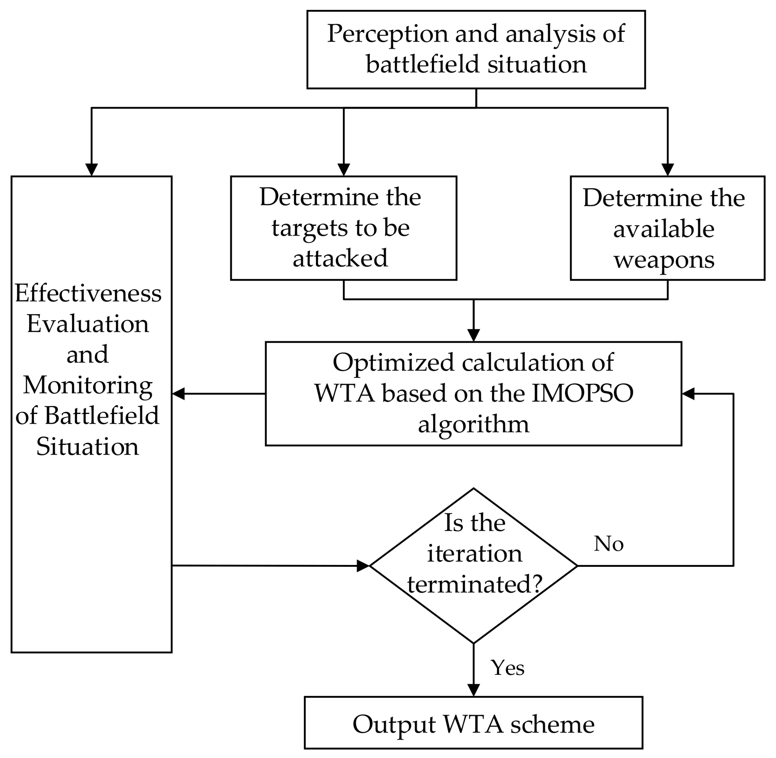
4.2.1. Decision-Making Process of DWTA Problem

Figure 3 shows the decision-making process of the DWTA problem. We can see from the figure that DWTA decision-making needs to determine the targets to be attacked and available weapons at the current stage on the basis of the results of battlefield situation analysis. Then, the determined targets and weapons are input into the IMOPSO algorithm to perform optimization iteration to obtain WTA decision. DWTA decision-making process also needs to evaluate and monitor the allocation results and battlefield situation, and determine whether iteration needs to be continued in accordance with the effect of the allocation scheme and battlefield situation.

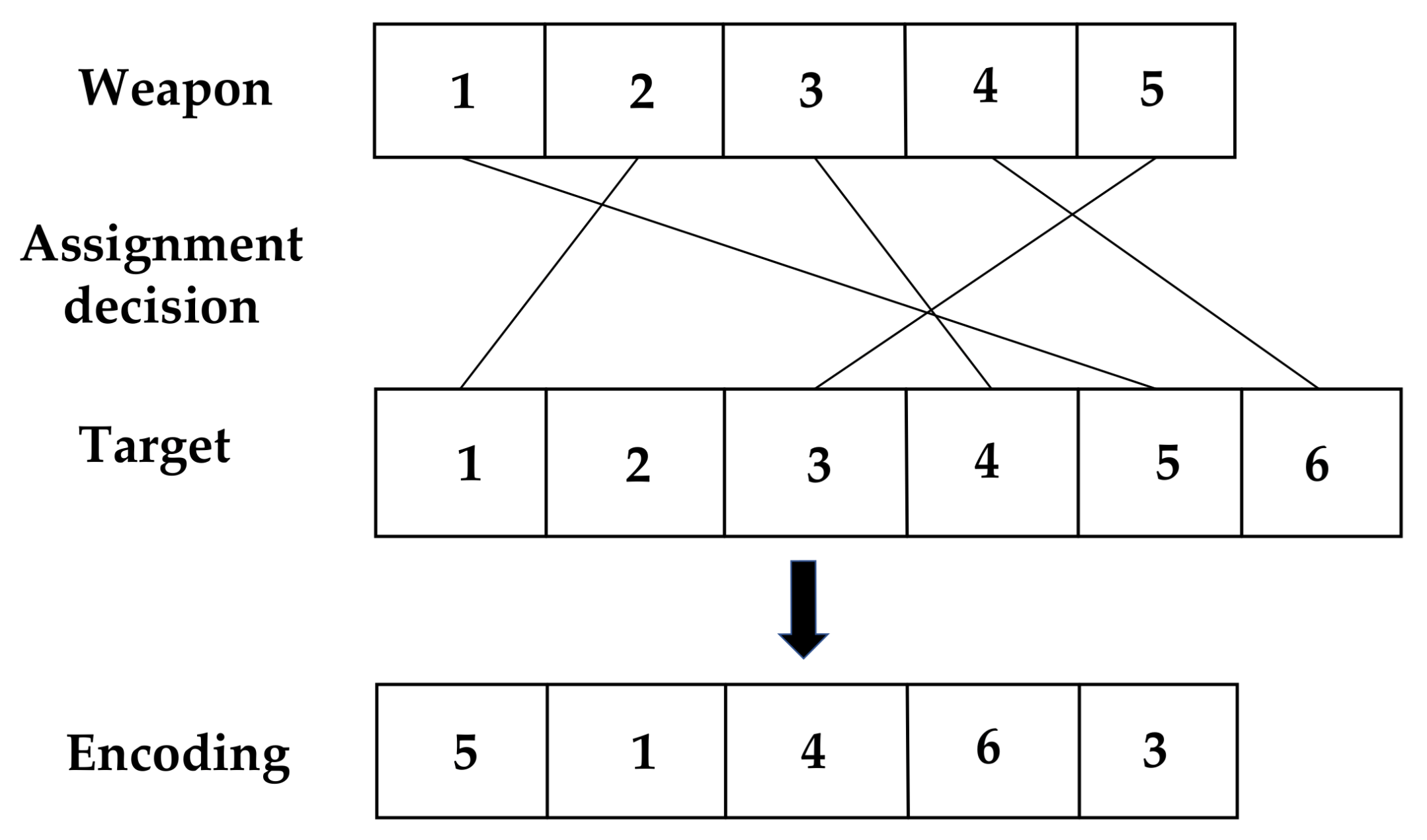
4.2.2. Integer Encoding Method

The allocation scheme obtained by IMOPSO algorithm in solving multiobjective DWTA can be obtained by decision matrix. To complete this process, we need to encode the particles. In order to obtain an efficient WTA scheme, the coding method can not only meet the solution of the model, but also meet the constraint requirements. Moreover, the encoding length should be made as small as possible. Based on the above conditions, this paper adopts integer encoding method. Take the following scenario ($W=5$, $T=6, S=1$) as an example to illustrate the coding method shown in Figure 4, where $\mathrm{X}$ is the corresponding decision matrix.

The decision matrix corresponding to the coding scheme is as follows:

$$X=\left[\begin{array}{cccccc}0& 0& 0& 0& 1& 0\\ 1& 0& 0& 0& 0& 0\\ 0& 0& 0& 1& 0& 0\\ 0& 0& 0& 0& 0& 1\\ 0& 0& 1& 0& 0& 0\end{array}\right]$$

4.2.3. Setting of Experimental Parameters

To verify the optimization performance of the IMOPSO algorithm in solving multiobjective DWTA problem, this section also uses IMOPSO, MOPSO, NSGA-II and MOEA/D for comparative analysis. Three different combat scenarios, i.e., small-, medium- and large-scaled cases are randomly generated in line with the number of weapons and targets. For each case, we generate the killing probability matrix $P\left(s\right)$, ammunition consumption matrix $U\left(s\right)$, feasibility matrix $F\left(s\right)$ and fire transferring feasibility matrix $FTF\left(s\right)$, and the elements in the matrix are randomly generated. The related parameters of DWTA problems are as follows: the number of weapons/targets/stages are 5/8/3, 15/24/5 and 30/50/8 in small/medium/large-scale cases, respectively. In all three cases, $n_i$ is 1, $N_i$ is 2. $m_j$ is 1 in small-scale case, and $m_j$ is 2 in medium-scale and large-scale case. The value vector of targets comes from Ref [40]. The number of iterations of all algorithms in the three scales are 100,150,200, respectively. The crossover probability and mutation probability of NSGA-II and MOEA/D are 0.9 and 0.1, respectively. Other parameters of the four algorithms are the same as those of solving the benchmark functions.

4.2.4. Performance Metrics

In this paper, the inverted generational distance ($IGD$) is used to measure the performance of multiobjective optimization algorithms in solving DWTA problem [41]. $IGD$ is a variant of $GD$, which can not only evaluate the convergence of multiobjective solutions, but also evaluate the distribution characteristics of solution set to a certain extent. The calculation formula is as follows:

$$IGD\left(P,P^{\ast }\right)\triangleq \frac{{{\displaystyle \sum }}_{i=1}^{\left|P^{\ast }\right|}dist\left(P_i^{\ast },P\right)}{\left|P^{\ast }\right|}$$

(21)

where $P^{\ast }$ is set of uniformly distributed points in the objective space along the true Pareto front (PF) or nearly true PF when it is hard or impossible to get the true PF, $P$ is an approximate PF of the true PF, $\left|P^{\ast }\right|$ represents the number of points in $P^{\ast }$, and $dist\left(P_i^{\ast },P\right)$ is the minimum Euclidean distance between $P_i^{\ast }$ and elements in $P$. The smaller the value of $IGD$, the better the convergence and distribution of the searched solution.

As to multiobjective DWTA problems, it is hard to obtain the true PF. To address this issue, we run each instance for 30 times, execute the non-dominated sorting on these solutions obtained earlier and select 500 evenly distributed points in Pareto front as the true Pareto front $P^{\ast }$.

5. Results

5.1. Simulation Results of Benchmark Functions

In order to eliminate the influence of the randomness of all algorithms on the simulation results, the four algorithms were independently run 30 times on all benchmark functions, and the results were statistically analyzed. The experimental results are shown in

Table 2. Comparison of the GD index of four algorithms.

Test Problems	Statistic	IMOPSO	MOPSO	NSGA-II	MOEA/D
SCH	max	8.2135 × 10−3	9.1342 × 10−3	8.9547 × 10−3	8.8592 × 10−3
	min	7.0125 × 10−3	6.9514 × 10−3	6.7452 × 10−3	7.5236 × 10−3
	ave	7.8253 × 10−3	8.2541 × 10−3	8.1023 × 10−3	8.0145 × 10−3
	std	2.1080 × 10−4	5.0172 × 10−4	5.0013 × 10−4	5.4671 × 10−4
FON	max	1.5231 × 10−3	3.8547 × 10−3	2.6321 × 10−3	2.8215 × 10−3
	min	1.0258 × 10−3	1.8569 × 10−3	1.8453 × 10−3	1.6329 × 10−3
	ave	1.2473 × 10−3	2.5146 × 10−3	2.2514 × 10−3	2.1397 × 10−3
	std	1.1545 × 10−4	4.3776 × 10−4	2.9165 × 10−4	1.6259 × 10−4
KUR	max	1.2663 × 10−1	5.9534 × 10−2	1.3012 × 10−2	1.9458 × 10−2
	min	5.3247 × 10−3	2.6536 × 10−2	9.8574 × 10−3	9.5847 × 10−3
	ave	1.0752 × 10−2	4.0853 × 10−2	1.1532 × 10−2	1.2532 × 10−2
	std	2.1964 × 10−2	8.4175 × 10−3	7.7454 × 10−4	1.9686 × 10−3
ZDT1	max	8.2362 × 10−4	1.6213 × 10−2	4.3132 × 10−3	5.8247 × 10−3
	min	3.0381 × 10−4	3.9211 × 10−4	2.0014 × 10−3	1.4356 × 10−3
	ave	5.8370 × 10−4	9.5527 × 10−4	2.1165 × 10−3	3.1143 × 10−3
	std	8.5002 × 10−5	2.1325 × 10−3	5.8285 × 10−4	8.2006 × 10−4
ZDT2	max	5.2434 × 10−4	9.2800 × 10−4	5.9324 × 10−3	8.3252 × 10−3
	min	3.3372 × 10−4	0.0000 × 10−4	1.8478 × 10−3	3.6892 × 10−4
	ave	3.6052 × 10−4	4.1485 × 10−4	3.4657 × 10−3	3.3358 × 10−3
	std	3.5078 × 10−5	1.9041 × 10−4	1.0549 × 10−4	2.3145 × 10−4
ZDT3	max	1.1263 × 10−4	1.2586 × 10−3	2.3123 × 10−3	5.2532 × 10−2
	min	5.5677 × 10−4	7.4425 × 10−4	1.5547 × 10−3	5.7817 × 10−4
	ave	7.8125 × 10−4	9.4334 × 10−4	1.8564 × 10−3	3.2984 × 10−3
	std	9.7499 × 10−5	1.4741 × 10−4	1.9552 × 10−4	9.5547 × 10−3
ZDT4	max	5.0733 × 10−4	2.2014 × 101	1.4857 × 10−3	1.4225 × 10−3
	min	3.7921 × 10−4	1.1057 × 10−2	5.2122 × 10−4	3.5120 × 10−4
	ave	4.5216 × 10−4	5.6523 × 100	8.6015 × 10−4	5.6826 × 10−4
	std	3.3182 × 10−5	6.4916 × 100	2.4718 × 10−4	1.9736 × 10−4
ZDT6	max	5.4012 × 10−3	1.4771 × 10−1	4.8123 × 10−2	3.3601 × 10−2
	min	2.5875 × 10−4	2.5815 × 10−4	2.5027 × 10−4	2.6774 × 10−4
	ave	4.6869 × 10−4	1.7124 × 10−2	1.9012 × 10−3	1.7445 × 10−3
	std	9.2828 × 10−4	4.3962 × 10−2	8.7443 × 10−3	6.2142 × 10−3

,

Table 3. Comparison of the $\mathsf{\Delta }$ index of four algorithms.

Test Problems	Statistic	IMOPSO	MOPSO	NSGA-II	MOEA/D
SCH	max	0.1684	0.8089	0.4020	0.7029
	min	0.0942	0.6745	0.2954	0.6893
	ave	0.1310	0.7377	0.3397	0.6941
	std	0.0183	0.0346	0.0278	0.0035
FON	max	0.2190	0.7685	0.3380	0.3383
	min	0.1522	0.5490	0.2519	0.1393
	ave	0.1755	0.6445	0.2960	0.1890
	std	0.0193	0.0455	0.0416	0.0201
KUR	max	0.4962	0.8775	0.5481	0.7487
	min	0.2707	0.6576	0.3756	0.6577
	ave	0.3218	0.7734	0.4248	0.6718
	std	0.0492	0.0603	0.0304	0.0212
ZDT1	max	0.1748	1.2275	0.3299	1.0560
	min	0.0953	0.6901	0.2371	0.2903
	ave	0.1309	0.8506	0.2809	0.3756
	std	0.0222	0.1009	0.0252	0.1973
ZDT2	max	0.2929	1.0000	0.3274	1.3130
	min	0.1003	0.6543	0.2331	0.1592
	ave	0.1432	0.8423	0.2804	0.6334
	std	0.0385	0.1005	0.0252	0.4185
ZDT3	max	0.7390	1.0942	0.5778	1.2469
	min	0.4399	0.8917	0.4929	0.8761
	ave	0.5124	1.0002	0.5304	0.9275
	std	0.0612	0.0480	0.0233	0.1033
ZDT4	max	0.1715	1.1476	0.3483	0.3942
	min	0.1023	0.6445	0.2496	0.2845
	ave	0.1359	0.8278	0.2946	0.2952
	std	0.0202	0.1018	0.0260	0.0217
ZDT6	max	1.3236	1.3701	1.1494	0.6851
	min	0.0695	0. 7524	0.2513	0.1336
	ave	0.1365	0.9291	0.3607	0.1573
	std	0.2248	0.1932	0.1814	0.0998

and

Table 4. Comparison of the DW index of four algorithms.

Test Problems	Statistic	IMOPSO	MOPSO	NSGA-II	MOEA/D
SCH	max	2.4265 × 10−3	1.0986 × 10−2	5.1149 × 10−3	1.2536 × 10−2
	min	2.9403 × 10−3	1.4418 × 10−4	4.0847 × 10−5	2.8466 × 10−4
	ave	6.0767 × 10−4	3.7421 × 10−3	1.0246 × 10−3	5.0172 × 10−3
	std	5.8435 × 10−4	3.4812 × 10−3	1.0683 × 10−3	3.4573 × 10−3
FON	max	9.7047 × 10−3	1.6692 × 10−2	1.0742 × 10−1	1.0283 × 10−2
	min	7.7566 × 10−6	5.8202 × 10−4	6.1194 × 10−5	1.1283 × 10−4
	ave	1.9247 × 10−3	5.1714 × 10−3	1.3052 × 10−2	2.9614 × 10−3
	std	2.2364 × 10−3	4.1587 × 10−3	2.0136 × 10−2	2.8547 × 10−3
KUR	max	6.5348 × 10−3	1.4637 × 10−1	7.1293 × 10−2	1.8347 × 10−1
	min	1.0722 × 10−4	7.1513 × 10−5	7.5517 × 10−4	3.0266 × 10−5
	ave	2.5493 × 10−3	2.0829 × 10−2	1.7056 × 10−2	1.1125 × 10−2
	std	1.7256 × 10−3	2.7645 × 10−2	1.9176 × 10−2	3.2862 × 10−2
ZDT1	max	4.1474 × 10−5	9.1931 × 10−1	2.2135 × 10−3	1.5789 × 100
	min	0.0000 × 100	1.1904 × 10−4	0.0000 × 100	0.0000 × 100
	ave	1.7483 × 10−6	8.7632 × 10−2	4.8683 × 10−4	6.5213 × 10−2
	std	7.6347 × 10−6	2.6313 × 10−1	4.9079 × 10−4	2.8732 × 10−1
ZDT2	max	4.8543 × 10−3	1.0000 × 100	5.4132 × 10−3	9.9673 × 10−1
	min	0.0000 × 100	0.0000 × 100	0.0000 × 100	3.9125 × 10−4
	ave	1.2353 × 10−3	2.9163 × 10−1	1.5364 × 10−3	3.4862 × 10−1
	std	1.0112 × 10−3	4.5072 × 10−1	1.5214 × 10−3	3.9228 × 10−1
ZDT3	max	9.8715 × 10−3	3.7582 × 10−1	2.1613 × 10−2	8.7073 × 10−1
	min	4.1056 × 10−6	5.9960 × 10−8	3.5787 × 10−6	1.0889 × 10−4
	ave	1.2125 × 10−3	1.8904 × 10−2	5.3247 × 10−3	3.2281 × 10−1
	std	2.0499 × 10−3	6.9826 × 10−2	4.6385 × 10−3	2.7195 × 10−1
ZDT4	max	1.0527 × 10−5	2.1396 × 101	1.7075 × 10−5	1.5036 × 10−2
	min	1.0527 × 10−5	6.7712 × 10−3	5.6429 × 10−6	4.2802 × 10−6
	ave	1.0527 × 10−5	6.6646 × 100	1.0759 × 10−5	7.1416 × 10−4
	std	4.9426 × 10−13	7.1038 × 100	2.2420 × 10−6	2.7158 × 10−3
ZDT6	max	5.5332 × 10−1	8.2603 × 100	5.1950 × 100	2.2690 × 100
	min	1.0593 × 10−8	9.9859 × 10−9	3.2261 × 10−7	6.0436 × 10−10
	ave	1.8572 × 10−2	1.0941 × 100	1.7324 × 10−1	1.0324 × 10−1
	std	1.0106 × 10−1	2.6645 × 100	9.4856 × 10−1	4.3597 × 10−1

, and the corresponding results of the maximum, minimum, mean and standard deviation are listed in above tables. The best results are bolded to facilitate the visualization.

Table 2 shows the statistical results of the $GD$ metric. It can be seen that the IMOPSO algorithm has obtained 28 optimal values out of 32 index statistics. For the function KUR, the $GD$ of IMOPSO has the largest standard deviation, which indicates that IMOPSO does not perform well in convergence stability. With respect to the other three algorithms, MOPSO has better convergence performance in functions ZDT1, ZDT2 and ZDT3, but its convergence stability is not as good as NSGA-II. MOEA/D has better performance in the $GD$ metric in functions ZDT4, ZDT6, SCH and FON than MOPSO and NSGA-II.

Table 3 shows the results of $∆$ indicator. We can see that IMOPSO has achieved the best average value in all eight test problems, which shows that the non-dominated solution generated by IMOPSO has the best distribution. However, it can be seen from the standard deviation of some functional indicators that IMOPSO is inferior to other algorithms in the $∆$ metric. The distribution performance of NSGA-II in the functions ZDT1, ZDT2 and ZDT3 is second only to that of IMOPSO. MOEA/D has obtained better $∆$ values in the functions ZDT4, ZDT6 and FON, while MOPSO has the worst $∆$ performance and has not gained any optimal value.

Table 4 is the statistical data of distribution width index $DW$. It can be seen from the data that IMOPSO is the best among the four algorithms except the minimum values of ZDT3, ZDT4, ZDT6 and KUR, and the data stability is also the best. The index performance of NSGA-II is second only to IMOPSO. Compared with MOPSO and MOEA/D, it has obtained the best values in functions ZDT1, ZDT2, ZDT3, ZDT4 and SCH, which implies that the solutions obtained by NSGA-II has the wider distribution range. MOEA/D performs well on functions ZDT6 and FON. The distribution width metric DW of MOPSO is still the worst among the four algorithms.

In order to show the ability of convergence to Pareto front more clearly, the comparison results of four algorithms for any one run of eight test problems are shown in Figure 5, Figure 6, Figure 7, Figure 8, Figure 9, Figure 10, Figure 11 and Figure 12.

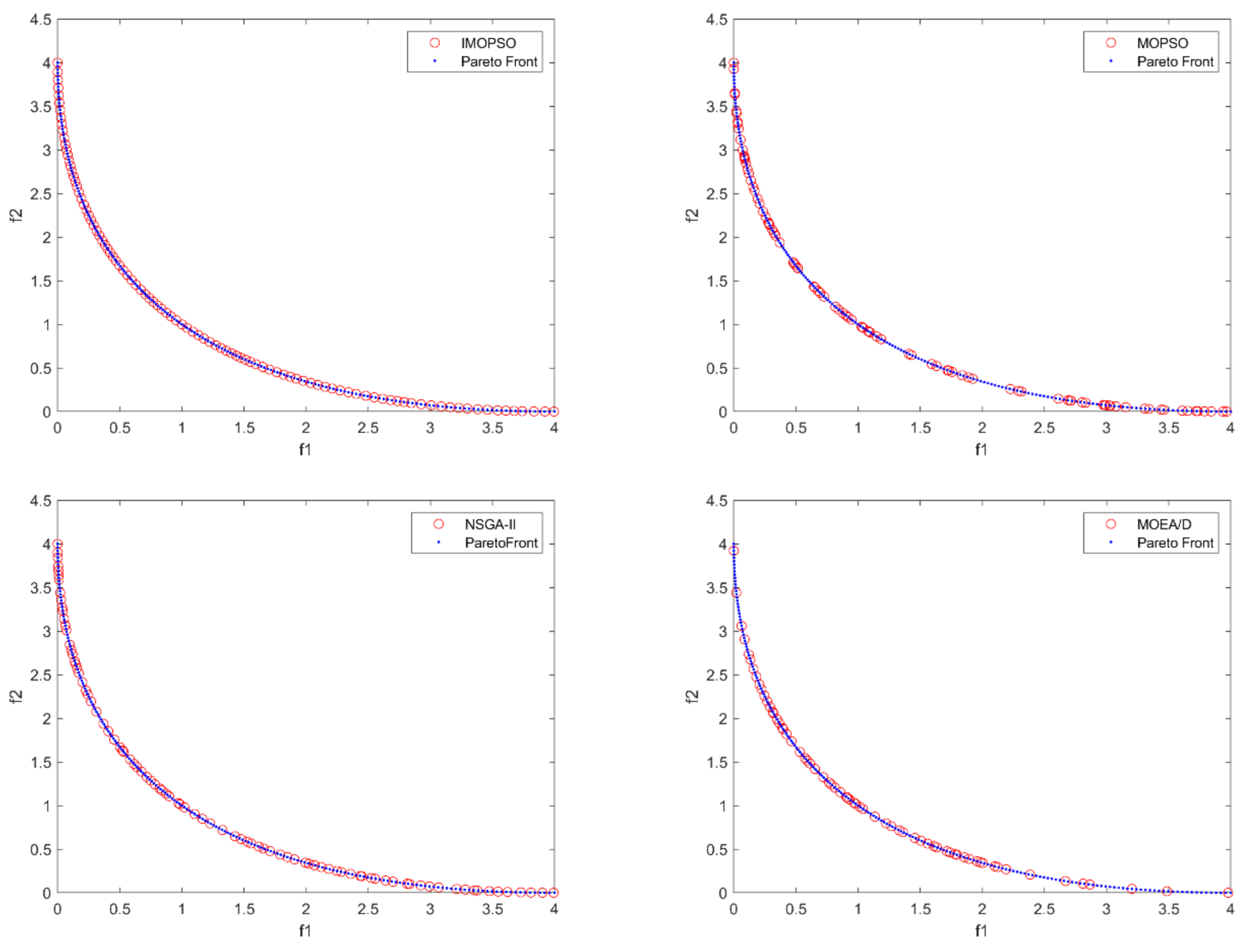
It can be seen from Figure 5 that the non-dominated solutions generated by IMOPSO are superior to the other three algorithms in both convergence and distribution. The solutions obtained by the other three algorithms can converge to the true PF, but the distribution of the solutions is poor, especially MOPSO and MOEA/D. It can be seen from the figure that many solutions cannot be searched, resulting in the solutions generated by the algorithms not covering the entire Pareto front. The performance of NSGA-II is second only to that of IMOPSO.

Figure 6 shows that the non-dominated solutions generated by the four algorithms can converge to the vicinity of the true PF. However, we can also find that the solution set generated by MOPSO and NSGA-II is not uniform enough and does not cover the entire Pareto front, which is also the reason for the poor statistical value of its distribution index. The distribution of the solution set obtained by MOEA/D is second only to that of IMOPSO. The solution set generated by IMOPSO has the best convergence and distribution among the four algorithms.

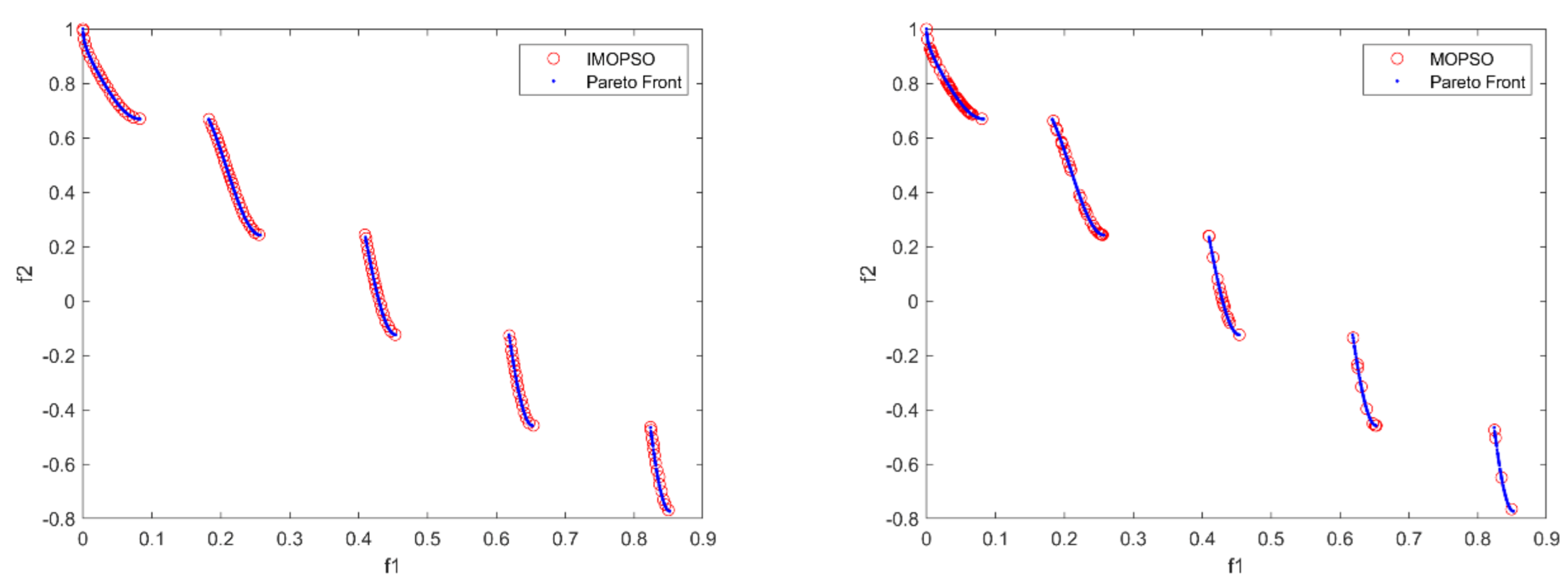
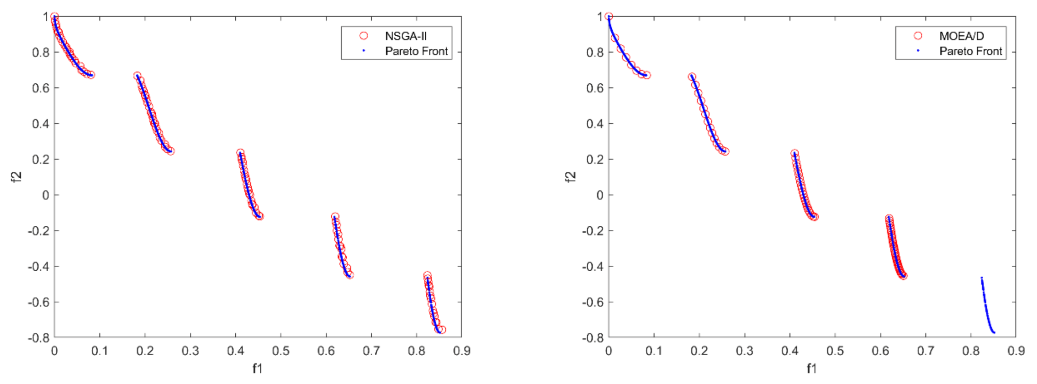
We can intuitively see from Figure 7 that the effect of MOPSO in solving KUR function is very poor. The non-dominated solutions obtained by MOPSO fail to converge to the true PF, and the solution set is not evenly distributed. The non-dominated solutions generated by NSGA-II and MOEA/D converge to the true PF. However, the solutions obtained by MOEA/D fail to cover the entire Pareto front, and the distribution of solutions is not as good as that of NSGA-II. IMOPSO is the best of the four algorithms.

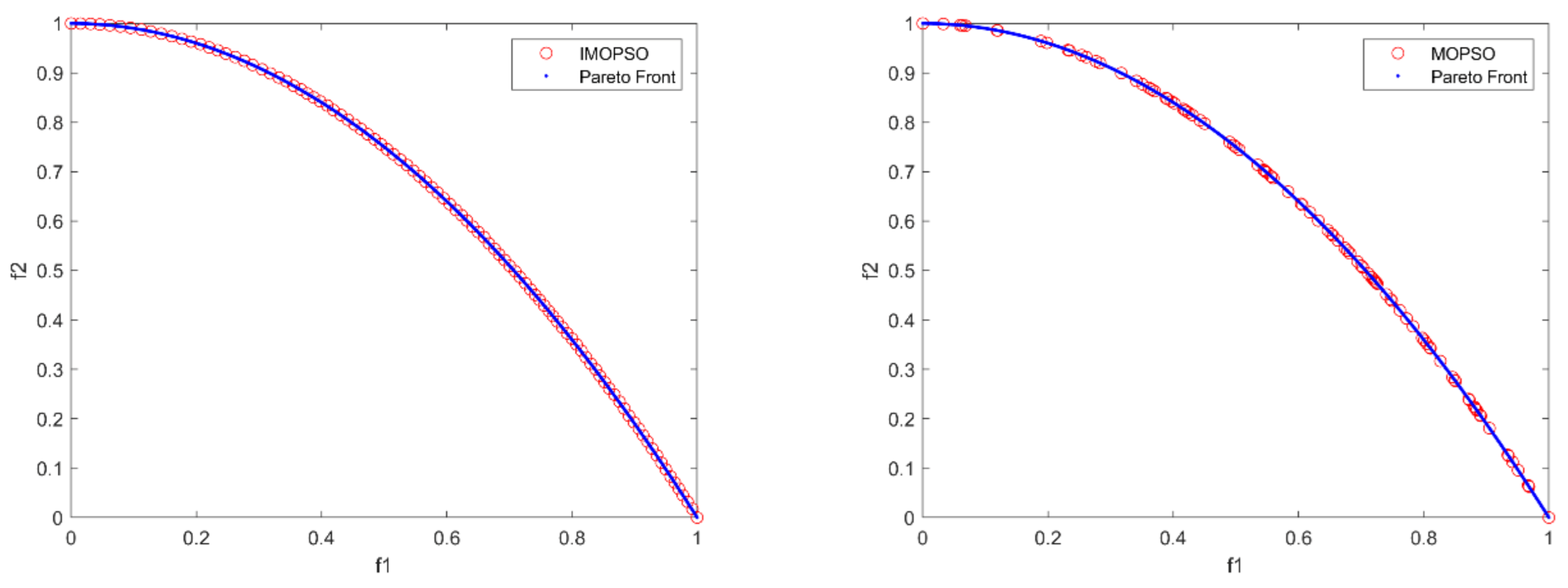
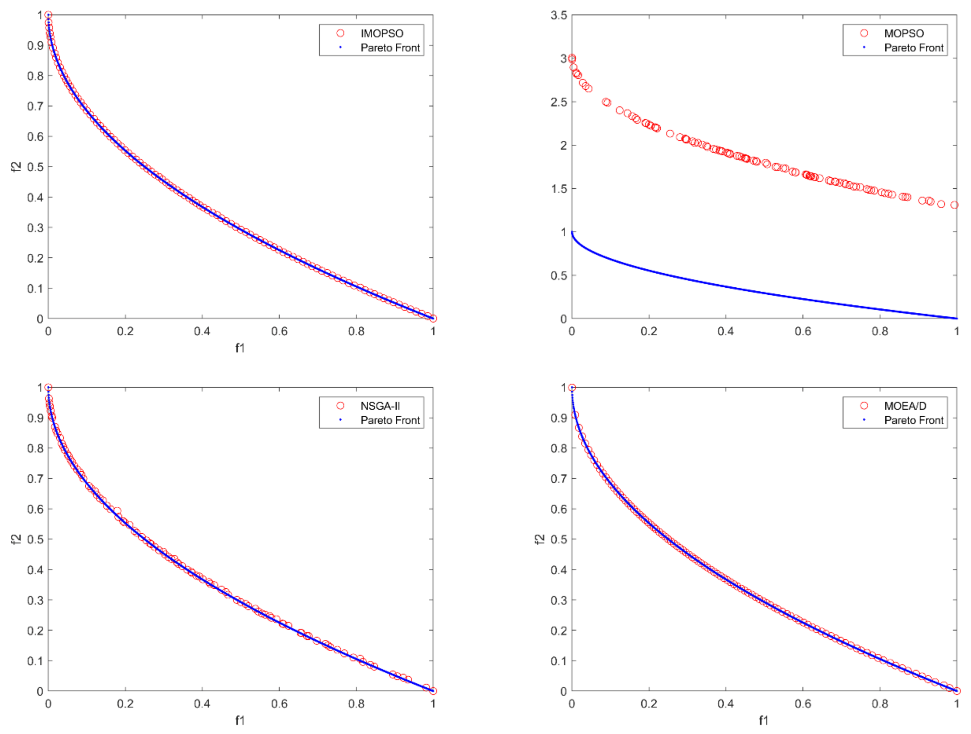
It can be seen from Figure 8 that the solutions obtained by IMOPSO and MOPSO converge to the true PF. The solution set generated by MOPSO is not evenly distributed and its distribution width is poor, and the non-dominated solutions solved by NSGA-II also exists the problem of uneven distribution. The convergence of MOEA/D is poor, and many solutions deviate from the true PF. IMOPSO is superior to the other three algorithms in both convergence and distribution.

Figure 9 indicates that the performance of the three metrics of the non-dominated solutions set generated by IMOPSO is the best. The non-dominated solution set generated by MOPSO can converge to the true PF, but the solutions distribution is poor. Compared with IMOPSO, NSGA-II also has the weakness of poor solutions distribution. The non-dominated solutions obtained by MOEA/D deviate from the true PF, especially in the later stage.

Figure 10 shows that the solution set generated by IMOPSO is superior to the other three algorithms in both convergence and distribution. The non-dominated solutions obtained by MOPSO can converge to the true PF, but the distribution of the solutions is uneven. There are cases where MOPSO fails to find the non-dominant solutions. The solution set generated by NSGA-II deviates slightly from the true PF, but it can be seen from the distribution of solutions that NSGA-II is better than MOPSO and MOEA/D. MOEA/D fails to search the complete Pareto front effectively, which is one of the reasons why the solution set generated by MOEA/D is poorly distributed.

Figure 11 indicates the distribution of solution sets generated by the four algorithms. IMOPSO is the best among the four algorithms in terms of convergence and distribution. The non-dominated solutions generated by MOPSO is far away from the true PF, and its performance in solving this problem is very poor. Non-dominated solutions generated by NSGA-II and MOEA/D can converge to the true PF, and the distribution characteristics of solutions obtained by MOEA/D are better than those of NSGA-II, which is mainly manifested in the relatively uniform distribution of solutions.

We can intuitively see from Figure 12 that both IMOPSO and MOEA/D have obtained solutions with excellent convergence and distribution, but IMOPSO performs better than MOEA/D. Non-dominated solutions solved by NSGA-II all converge to the true PF, but the distribution of solutions is not as uniform as MOEA/D. The solutions generated by MOPSO also converge to the true PF, but the distribution of the solution is poor, and many solutions are not found.

5.2. Simulation Results of the DWTA Problem

For three DWTA problems of different scales (small, medium and large), four algorithms, i.e., IMOPSO, MOPSO, NSGA-II and MOEA/D, are used to solve them respectively. Each algorithm runs independently for 30 times. The experimental results are shown in the

Table 5. Comparison of the IGD index of four algorithms.

Cases	Statistic	IMOPSO	MOPSO	NSGA-II	MOEA/D
Small	max	2.0899	4.4919	3.7781	18.5805
	min	0.1794	0.7148	0.4456	9.3359
	ave	0.5871	1.5536	1.4704	11.6643
	std	0.4426	0.9613	0.8294	2.2159
Medium	max	7.1089	11.7417	7.1093	38.1172
	min	2.4670	2.2153	1.3007	29.3465
	ave	3.2486	6.4850	3.7795	32.1274
	std	1.1570	3.0458	1.2904	2.1213
Large	max	7.1926	12.7778	9.8487	87.5192
	min	2.7628	3.1651	3.0999	64.7363
	ave	4.3028	6.2359	5.2511	73.0749
	std	1.0646	2.0957	1.4718	6.0825

.

It can be seen from the results in Table 5 that the IMOPSO algorithm has achieved the best $IGD$ values in all three instances, and it indicates that IMOPSO has better performance than the other three algorithms in solving multiobjective DWTA problems. With the increase of the scale of DWTA problems, the non-dominated solutions generated by IMOPSO also obtain excellent convergence and distribution. The performance of NSGA-II in solving multiobjective DWTA issues is second only to that of IMOPSO, especially in medium scale, and the statistical values of NSGA-II are very close to that of IMOPSO. MOPSO has little difference with NSGA-II in small-scale and large-scale instance, and its overall performance is second only to NSGA-II. The effect of MOEA/D in solving DWTA problems is very poor. Its index values are far behind the other three algorithms, and this gap is becoming more and more obvious with the increase of the problem scale. This is due to the strictness of the five constraints in the multiobjective DWTA problem discussed in this paper, which leads to the increased difficulty of solving the model. Moreover, MOEA/D needs to normalize the objectives when dealing with multiobjective DWTA problems, so the computational complexity is greatly increased.

To visually compare the abilities of the four algorithms in solving multiobjective DWTA problems of three scales, we give the comparison results between the solution sets generated by any one run of the four algorithms at each scale and the true PF, and the comparison results are shown in Figure 13, Figure 14, Figure 15, Figure 16, Figure 17 and Figure 18.

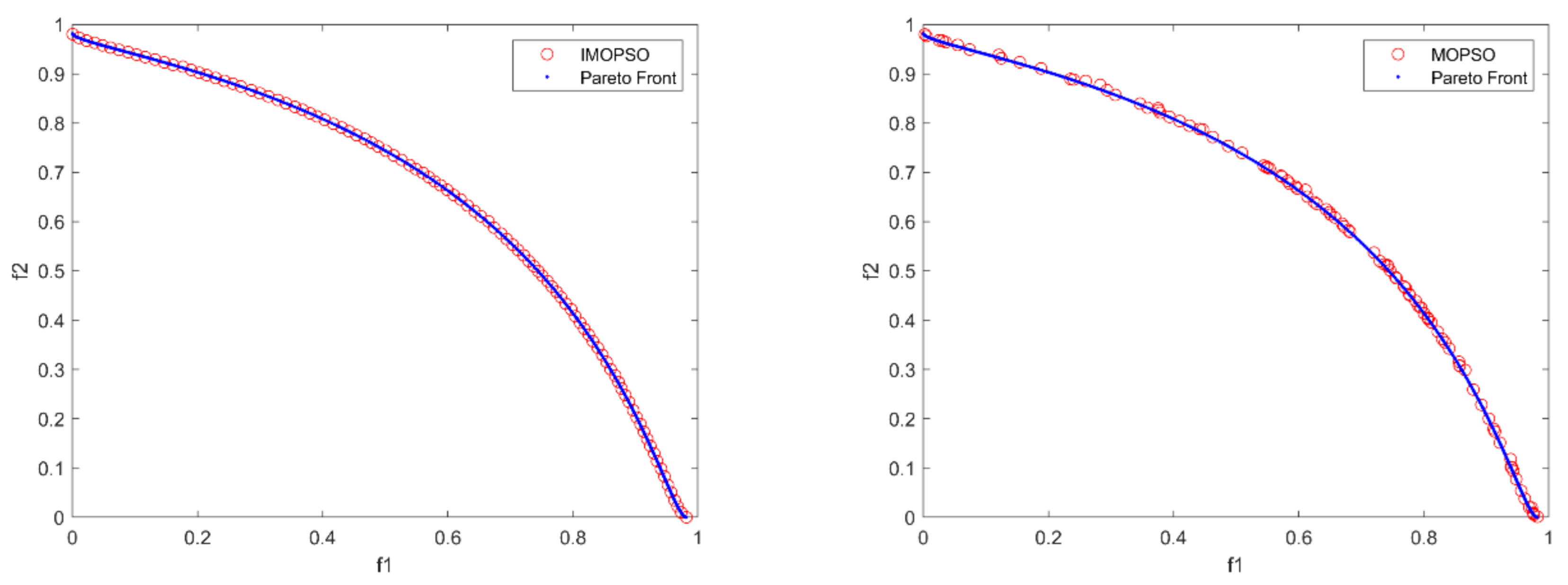
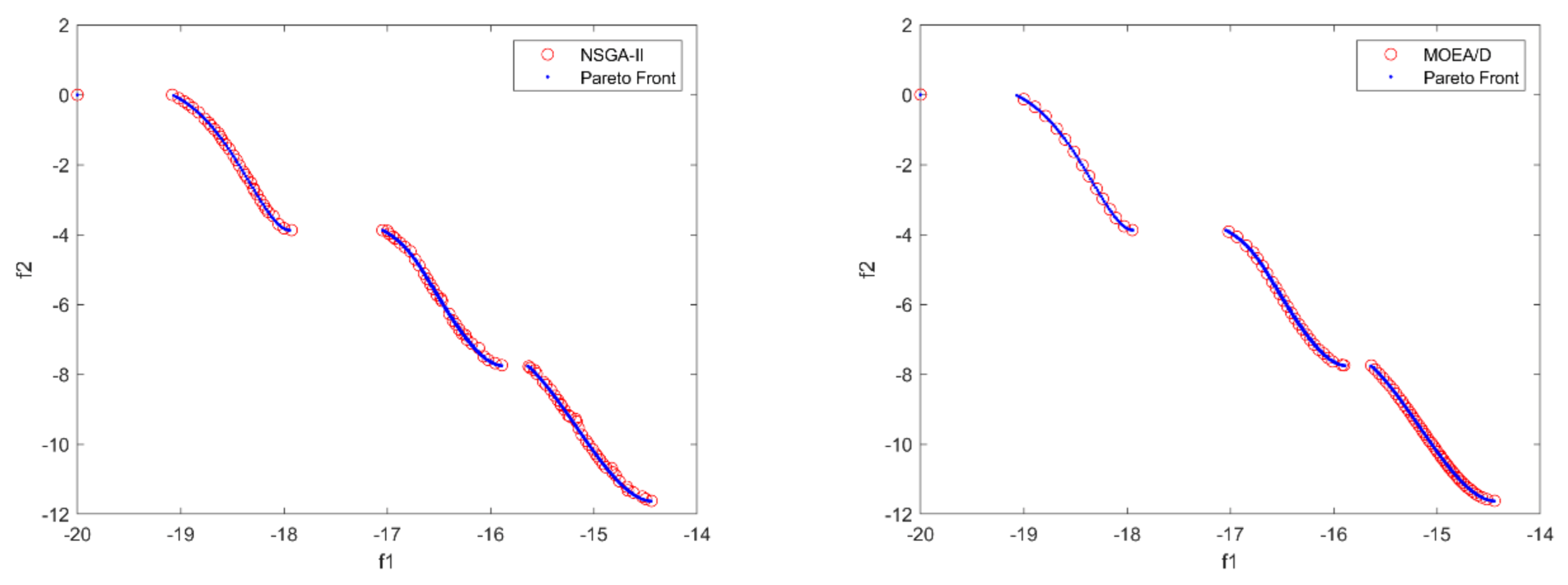
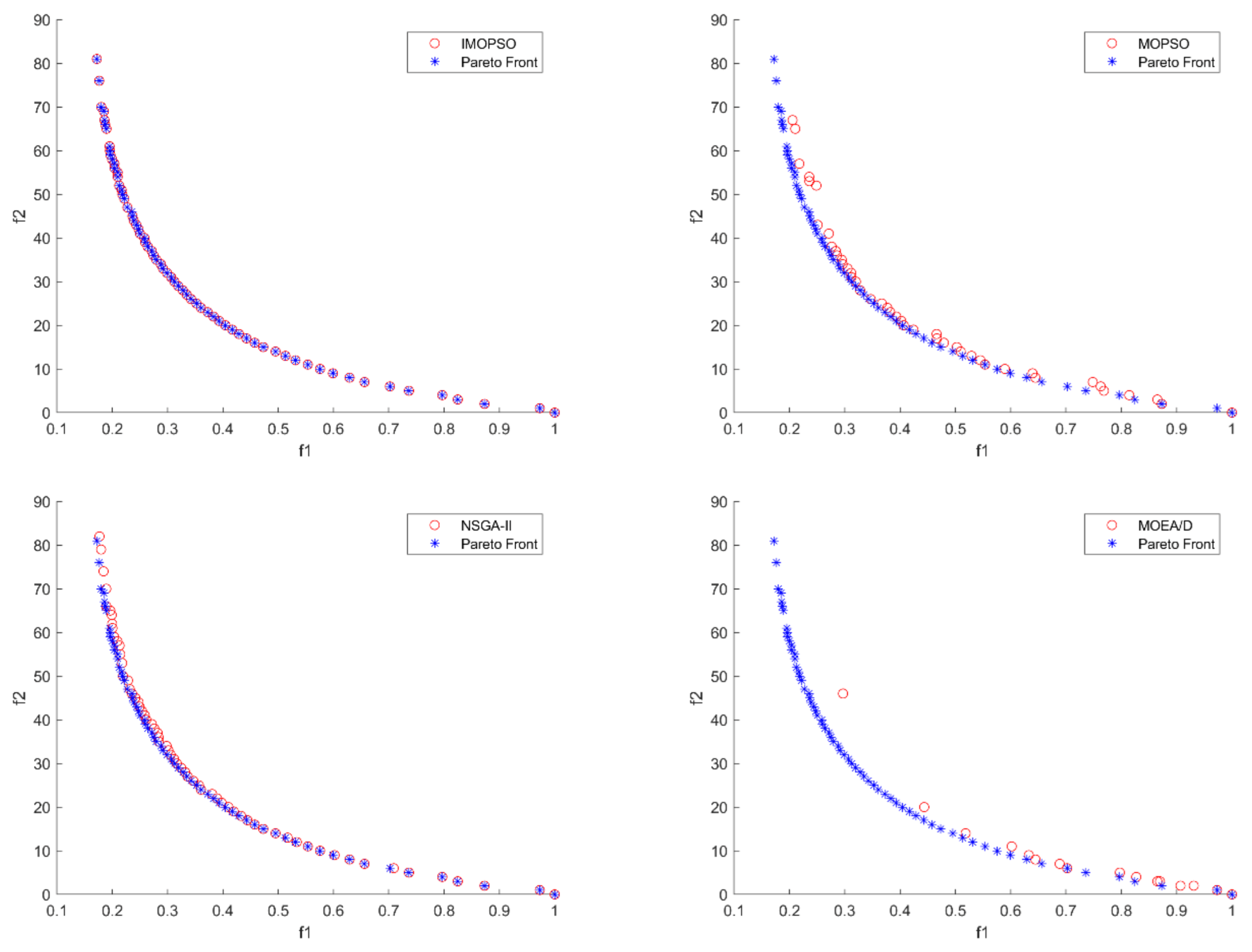
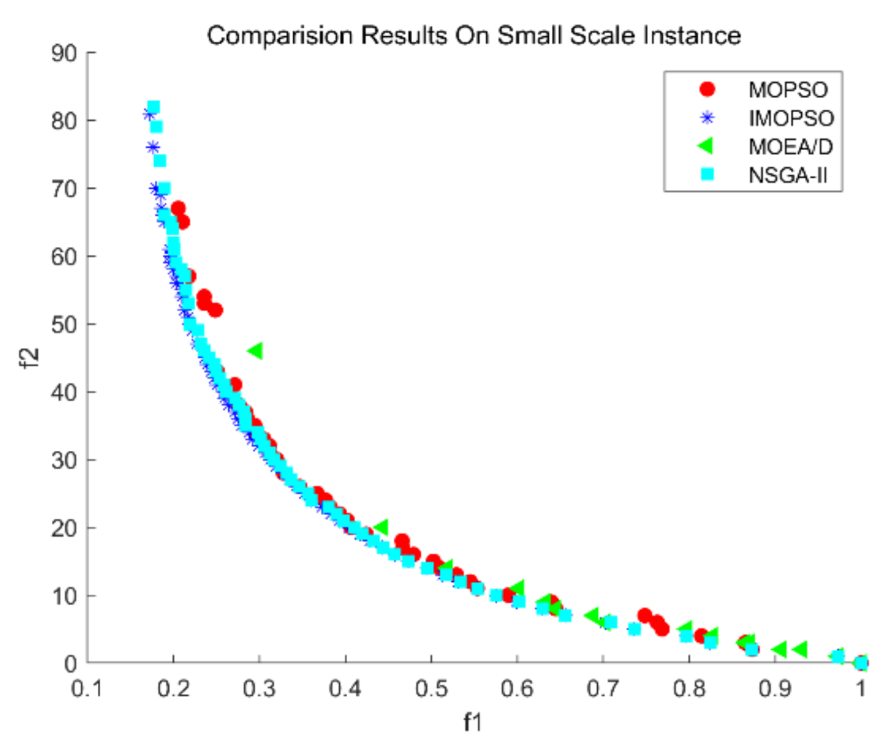
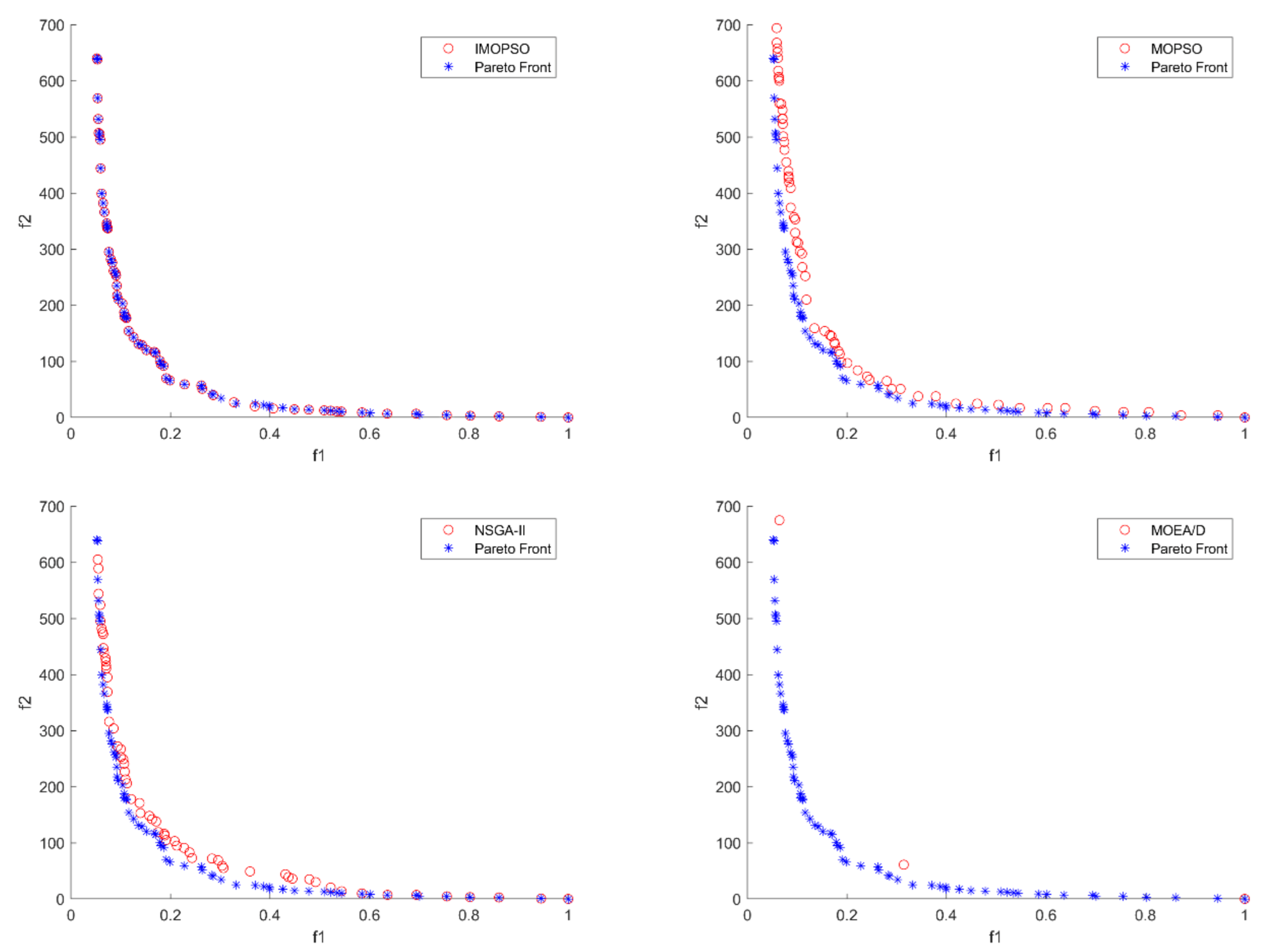
It can be seen by Figure 13 and Figure 14 that IMOPSO performs very well in solving small-scale multiobjective DWTA problem, and the solutions obtained by IMOPSO can converge to the true PF. The solutions obtained by MOPSO failed to converge to the true PF, and the distribution of the solution set is poor, which failed to completely cover the entire Pareto front. NSGA-II is second only to IMOPSO, and its non-dominated solutions mostly converge to Pareto front. MOEA/D is the worst one, which almost obtain no useful Pareto solutions.

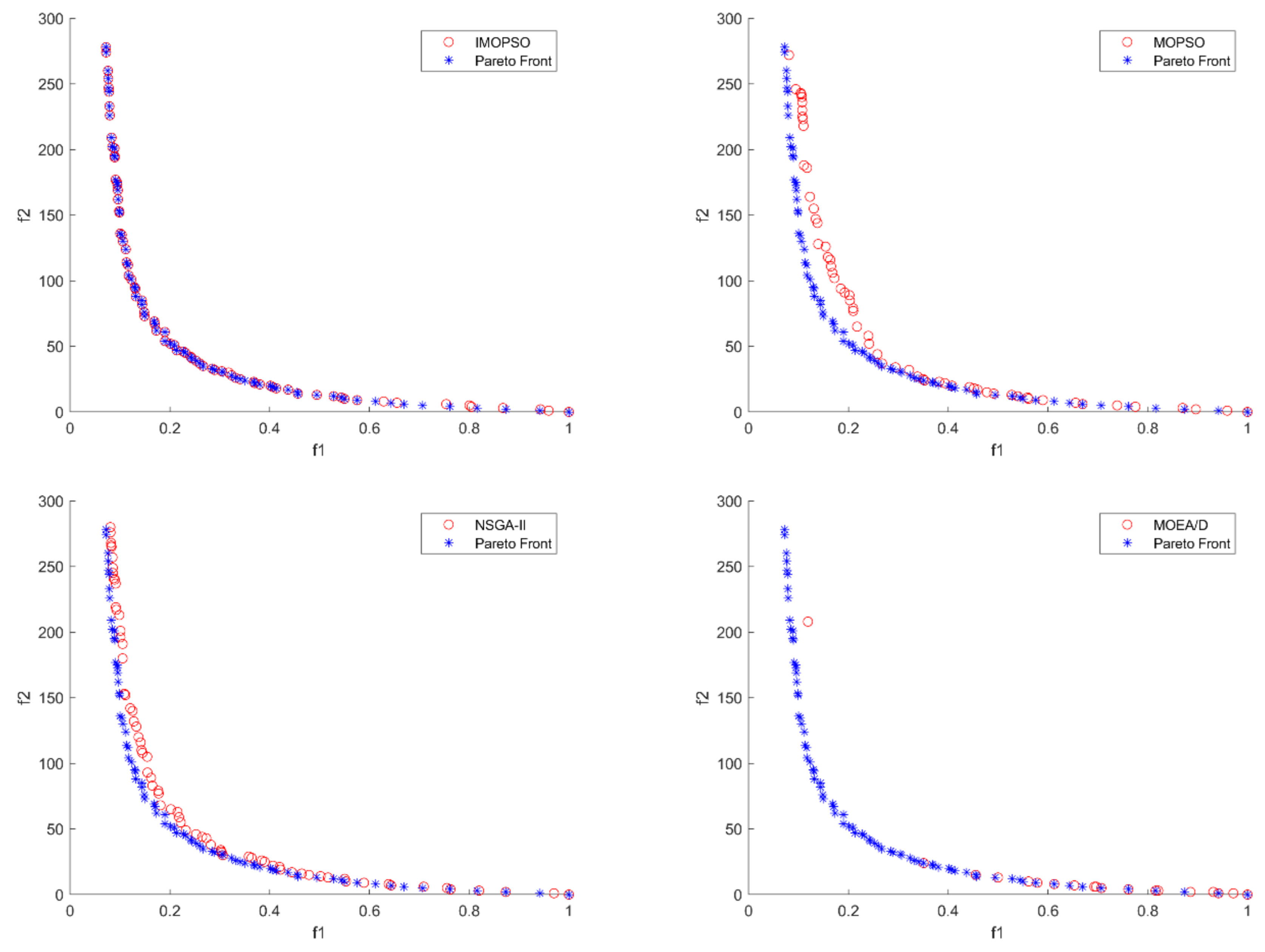
Figure 15 and Figure 16 show the distribution comparison of solution sets of four algorithms in medium scale. It can be seen that most of the solutions obtained by IMOPSO converge to the true PF, and only a few solutions fail to fall on the Pareto front. The non-dominated solutions generated by NSGA-II have a distance from true PF, and its convergence is far less than that of IMOPSO. Compared with NSGA-II, the solution set obtained by MOPSO is farther from the true PF. MOEA/D is the worst among the four algorithms, which generates very few solutions, and the solution set cannot completely cover the entire Pareto front.

Figure 17 and Figure 18 are the comparison results of four algorithms for solving large-scale multiobjective DWTA problem. It can be seen that the set of non-dominated solutions obtained by IMOPSO for solving large-scale multiobjective DWTA problem can fully converge to the Pareto front, and most of the non-dominated solutions have the same values as the solutions of true PF. Some solutions generated by NSGA-II can converge to the true PF, but there is still a distance from the Pareto front in the middle location. The solution set obtained by MOPSO fails to converge to the true PF, but the distribution of solutions is relatively good. MOEA/D only finds three solutions. It can be seen that with the increase of DWTA problem scale, MOEA/D is getting worse and worse.

6. Discussion

In order to evaluate the improved multiobjective particle swarm optimization algorithm proposed in this paper, we conducted two sets of comparative experiments with three multiobjective optimization algorithms, i.e., IMOPSO, NSGA-II and MOEA/D. According to the experimental results of benchmark functions, the IMOPSO algorithm proposed in this paper has achieved the best values in all three evaluation indexes, which shows that the solutions obtained by IMOPSO in solving MOPs have better convergence and distribution. Through the solution set distribution graphs, we can also intuitively see the superiority of IMOPSO in solving MOPs compared with the other three algorithms. The results in the figure just correspond to the statistical data of the evaluation index, which shows the rationality of the data. Comparative experiments of multiobjective DWTA problems show that IMOPSO algorithm can also solve satisfactory solutions with the increasing scale of DWTA problems, thus obtaining an effective weapon-target allocation scheme. The results of solving the multiobjective DWTA problem reflect the ability of IMOPSO in dealing with practical MOPs, which shows that IMOPSO algorithm is more suitable for solving large-scale mixed integer programming problems than other algorithms.

We use the average value of each performance metric in the experiment to measure the improvement degree of IMOPSO compared with other algorithms of dealing with MOPs. The specific method is as follows: We sum the metric average values of each benchmark function, and then find the average value as the comprehensive index value. The DWTA problem also adopts the same processing method. Through the calculation, we can conclude that IMOPSO is superior to MOPSO, NSGA-II and MOEA/D in GD/Δ/DW/IGD index, which are 99.61%/74.46%/99.68%/42.99%, 29.97%/39.90%/87.67%/22.50%, 35.33%/57.22%/96.96%/93.04%, respectively. It can be seen from the above values that the improved effect of the proposed IMOPSO algorithm on the basis of MOPSO algorithm is particularly remarkable, and the performance of IMOPSO in solving MOPs is also significantly ahead of NSGA-II and MOEA/D. IMOPSO can be regarded as the best of the four algorithms, which successfully overcomes the shortcoming that MOPSO is easy to fall into local optimum, and can also balance the contradiction between exploration and exploitation. Experimental results show that compared with other algorithms, IMOPSO is not only more robust and accurate, but also has a wide range of applications, which is more suitable for dealing with complex MOPs.

Although the IMOPSO algorithm has many excellent performances, it is not completely flawless when dealing with MOPs. At first, the number of times that the IMOPSO algorithm needs to call the objective function in each iteration is very large. Since the benchmark functions have simple and clear mathematical expressions, it is not an insurmountable problem for the optimization system itself to call the objective function more times. However, many problems that need to be solved in engineering application are “black box” types, which cannot be directly expressed by mathematical formulas. This requires huge computer resources as support, so it is necessary to properly handle them in the optimization program. Secondly, in this paper, it is difficult to determine the specific number of unimproved generations when the $g_{best}$ proceeds mutation operation, so we conducted many experiments to determine it.

7. Conclusions and Future Works

To solve the multiobjective DWTA problem effectively, a novel MOPSO algorithm (IMOPSO) is proposed in this paper. The algorithm constructs different learning strategies for dominated and non-dominated solutions in the current population, which makes the learning pertinence of particles clearer. IMOPSO adopts a search strategy based on SBX and PM. The exchange of information among particles is enhanced by the SBX operator of $p_{best}$ in external archive, and the PM operation is performed on newly generated $g_{best}$, thereby generating new global optimal particles. SBX and PM address the drawback that MOPSO algorithm is easy to fall into local optimal solution. The algorithm also uses a dynamic external archive maintenance strategy, which improves the diversity of non-dominated solutions. Two sets of experiments based on benchmark functions and multiobjective DWTA problem are used to verify the performance of IMOPSO. In order to illustrate the effectiveness of IMOPSO in solving MOPs, we compared three state-of-the-art multiobjective optimization algorithms: MOPSO, NSGA-II and MOEA/D. The experimental results show that the non-dominated solution obtained by the proposed IMOPSO algorithm is superior to other algorithms in convergence and distribution. Furthermore, IMOPSO has advantages in solving large-scale mixed integer programming problems.

The benchmark functions and multiobjective DWTA model selected in this paper only have two objectives. In reality, there are often more optimization objectives in optimization problems. In the future, we will use more types of benchmark functions which include more objectives to verify the ability of the IMOPSO algorithm. In addition, IMOPSO will be used to solve more multiobjective optimization problem models. Moreover, we will compare IMOPSO with more intelligent algorithms. At present, there are many solvers for multiobjective optimization models, and we will use other solvers (e.g., Gurobi and CPLEX) to solve DWTA problems in future research.

References

- Day, R.H. Allocating weapons to target complexes by means of nonlinear programming. Oper. Res. 1966, 14, 992–1013. [Google Scholar] [CrossRef]
- Lee, M.-Z. Constrained Weapon–Target Assignment: Enhanced Very Large Scale Neighborhood Search Algorithm. IEEE Trans. Syst. Man Cybern. Part A. Syst. Hum. A Publ. IEEE Syst. Man Cybern. Soc. 2010, 40, 198–204. [Google Scholar] [CrossRef]
- Bogdanowicz, Z.R. Advanced Input Generating Algorithm for Effect-Based Weapon–Target Pairing Optimization. IEEE Trans. Syst. Man Cybern. Part A. Syst. Hum. A Publ. IEEE Syst. Man Cybern. Soc. 2012, 42, 276–280. [Google Scholar] [CrossRef]
- Bogdanowicz, Z.R.; Tolano, A.; Patel, K.; Coleman, N.P. Optimization of Weapon–Target Pairings Based on Kill Probabilities. IEEE Trans. Cybern. 2013, 43, 1835–1844. [Google Scholar] [CrossRef] [PubMed]
- Bogdanowicz, Z.R.; Patel, K. Quick Collateral Damage Estimation Based on Weapons Assigned to Targets. IEEE Trans. Syst. Man Cybern. Syst. 2015, 45, 762–769. [Google Scholar] [CrossRef]
- Şahin, M.A.; Leblebicioğlu, K. Approximating the optimal mapping for weapon target assignment by fuzzy reasoning. Inf. Sci. 2014, 255, 30–44. [Google Scholar] [CrossRef]
- Kline, A.; Ahner, D.; Hill, R. The Weapon-Target Assignment Problem. Comput. Oper. Res. 2019, 105, 226–236. [Google Scholar] [CrossRef]
- Kalmár-Nagy, T.; Giardini, G.; Bak, B.D. The multiagent planning problem. Complexity 2017, 2017, 3813912. [Google Scholar] [CrossRef]
- Hosein, P.A.; Athans, M. Preferential Defense Strategies. Part I: The Static Case (Technical Report); LIPS-P-2002; MIT Lab. Inf. Decis. Syst.: Cambridge, MA, USA, 1990. [Google Scholar]
- Hocaoglu, M.F. Weapon Target Assignment Optimization for Land based Multi-Air Defense Systems: A Goal Programming Approach. Comput. Ind. Eng. 2019, 128, 681–689. [Google Scholar] [CrossRef]
- Yao, Z.; Li, M.; Chen, Z.; Rui, Z. Mission decision-making method of multi-aircraft cooperatively attacking multi-target based on game theoretic framework. Chin. J. Aeronaut. 2016, 29, 1685–1694. [Google Scholar] [CrossRef] [Green Version]
- Ni, M.; Yu, Z.; Feng, M.; Wu, X. A Lagrange Relaxation Method for Solving Weapon-Target Assignment Problem. Math. Probl. Eng. 2011, 2011, 264–265. [Google Scholar] [CrossRef] [Green Version]
- Hongtao, L.; Fengju, K. Adaptive chaos parallel clonal selection algorithm for objective optimization in WTA application. Opt.—Int. J. Light Electron Opt. 2016, 127, 3459–3465. [Google Scholar] [CrossRef]
- Sonuc, E.; Sen, B.; Bayir, S. A parallel simulated annealing algorithm for weapon-target assignment problem. Int. J. Adv. Comput. Sci. Appl. 2017, 8, 87–92. [Google Scholar] [CrossRef] [Green Version]
- Chen, J.; Xin, B.; Peng, Z.H.; Dou, L.H.; Zhang, J. Evolutionary decision-makings for the dynamic weapon-target assignment problem. Sci. China Ser. F Inf. Sci. 2009, 52, 2006. [Google Scholar] [CrossRef]
- Li, X.; Zhou, D.; Pan, Q.; Tang, Y.; Huang, J. Weapon-target assignment problem by multiobjective evolutionary algorithm based on decomposition. Complexity 2018, 2018, 8623051. [Google Scholar] [CrossRef]
- Hu, X.; Luo, P.; Zhang, X.; Wang, J. Improved ant colony optimization for weapon-target assignment. Math. Probl. Eng. 2018, 2018, 6481635. [Google Scholar] [CrossRef] [Green Version]
- Juan, L.I.; Jie, C.; Bin, X. Efficiently solving multi-objective dynamic weapon-target assignment problems by NSGA-II. In Proceedings of the 2015 34th Chinese Control Conference (CCC), Hangzhou, China, 28–30 July 2015; pp. 2556–2561. [Google Scholar]
- Li, J.; Chen, J.; Xin, B.; Dou, L. Solving multi-objective multi-stage weapon target assignment problem via adaptive NSGA-II and adaptive MOEA/D: A comparison study. In Proceedings of the 2015 IEEE Congress on Evolutionary Computation (CEC), Sendai, Japan, 25–28 May 2015; pp. 3132–3139. [Google Scholar]
- Li, J.; Chen, J.; Xin, B.; Chen, L. Efficient multi-objective evolutionary algorithms for solving the multi-stage weapon target assignment problem: A comparison study. In Proceedings of the 2017 IEEE Congress on Evolutionary Computation (CEC), Donostia, Spain, 5–8 June 2017; pp. 435–442. [Google Scholar]
- Li, Y.; Kou, Y.; Li, Z.; Xu, A.; Chang, Y. A modified pareto ant colony optimization approach to solve biobjective weapon-target assignment problem. Int. J. Aerosp. Eng. 2017, 2017, 1746124. [Google Scholar] [CrossRef] [Green Version]
- Zitzler, E.; Laumanns, M.; Thiele, L. SPEA2: Improving the Strength Pareto Evolutionary Algorithm. In Proceedings of the EUROGEN 2001 Evolutionary Methods for Design, Optimization and Control with Applications to Industrial Problems, Athens, Greece, 19–21 September 2001. [Google Scholar]
- Corne, D.W.; Jerram, N.R.; Knowles, J.D.; Oates, M.J. PESA-II: Region-based selection in evolutionary multiobjective optimization. In Proceedings of the 3rd Annual Conference on Genetic and Evolutionary Computation, San Francisco, CA, USA, 7–11 July 2001; pp. 283–290. [Google Scholar]
- Deb, K.; Pratap, A.; Agarwal, S.; Meyarivan, T.A.M.T. A fast and elitist multiobjective genetic algorithm: NSGA-II. IEEE Trans. Evol. Comput. 2002, 6, 182–197. [Google Scholar] [CrossRef] [Green Version]
- Zhang, Q.; Li, H. MOEA/D: A multiobjective evolutionary algorithm based on decomposition. IEEE Trans. Evol. Comput. 2007, 11, 712–731. [Google Scholar] [CrossRef]
- Coello, C.A.C.; Pulido, G.T.; Lechuga, M.S. Handling multiple objectives with particle swarm optimization. IEEE Trans. Evol. Comput. 2004, 8, 256–279. [Google Scholar] [CrossRef]
- Li, X. A non-dominated sorting particle swarm optimizer for multiobjective optimization. In Proceedings of the Genetic and Evolutionary Computation Conference, Chicago, IL, USA, 12–16 July 2003; Springer: Berlin/Heidelberg, Germany; pp. 37–48. [Google Scholar]
- Li, X. Better spread and convergence: Particle swarm multiobjective optimization using the maximin fitness function. In Proceedings of the Genetic and Evolutionary Computation Conference, Seattle, WA, USA, 26–30 June 2004; Springer: Berlin/Heidelberg, Germany; pp. 117–128. [Google Scholar]
- Raquel, C.R.; Naval, P.C., Jr. An effective use of crowding distance in multiobjective particle swarm optimization. In Proceedings of the 7th Annual Conference on Genetic and Evolutionary Computation, Washington, DC, USA, 25–29 June 2005; pp. 257–264.
- Santana, R.A.; Pontes, M.R.; Bastos-Filho, C.J.A. A multiple objective particle swarm optimization approach using crowding distance and roulette wheel. In Proceedings of the 2009 Ninth International Conference on Intelligent Systems Design and Applications, Pisa, Italy, 30 November–2 December 2009; pp. 237–242. [Google Scholar]
- Agrawal, S.; Dashora, Y.; Tiwari, M.K.; Son, Y.J. Interactive particle swarm: A Pareto-adaptive metaheuristic to multiobjective optimization. IEEE Trans. Syst. Man Cybern.-Part A Syst. Hum. 2008, 38, 258–277. [Google Scholar] [CrossRef]
- Abdullah, M.; Al-Muta’a, E.A.; Al-Sanabani, M. Integrated MOPSO algorithms for task scheduling in cloud computing. J. Intell. Fuzzy Syst. 2019, 36, 1823–1836. [Google Scholar] [CrossRef]
- Zhao, W.; Luan, Z.; Wang, C. Parameter optimization design of vehicle E-HHPS system based on an improved MOPSO algorithm. Adv. Eng. Softw. 2018, 123, 51–61. [Google Scholar] [CrossRef]
- Najimi, M.; Pasandideh, S.H.R. Modelling and solving a bi-objective single period problem with incremental and all unit discount within stochastic constraints: NSGAII and MOPSO. Int. J. Serv. Oper. Manag. 2018, 30, 520–541. [Google Scholar] [CrossRef]
- Lee, Z.J.; Su, S.F.; Lee, C.Y. Efficiently solving general weapon-target assignment problem by genetic algorithms with greedy eugenics. IEEE Trans. Syst. Man Cybern. Part B 2003, 33, 113–121. [Google Scholar]
- Lin, Q.; Li, J.; Du, Z.; Chen, J.; Ming, Z. A novel multi-objective particle swarm optimization with multiple search strategies. Eur. J. Oper. Res. 2015, 247, 732–744. [Google Scholar] [CrossRef]
- Zitzler, E.; Deb, K.; Thiele, L. Comparison of multiobjective evolutionary algorithms: Empirical results. Evol. Comput. 2000, 8, 173–195. [Google Scholar] [CrossRef] [Green Version]
- Van Veldhuizen, D.A.; Lamont, G.B. Evolutionary computation and convergence to a Pareto front. In Proceedings of the Late Breaking Papers at the Genetic Programming 1998 Conference, Stanford University, Stanford, CA, USA, 22–25 July 1998; pp. 221–228. [Google Scholar]
- Deb, K. Multiobjective Optimization Using Evolutionary Algorithms; John Wiley & Sons, Inc.: Hoboken, NJ, USA, 2001. [Google Scholar]
- Cui, H.B. Study on Firepower Optimal Distribution of Artillery Group Based on NSGA-I. Master’s Thesis, National University of Defense Technology, Changsha, China, 2010. (In Chinese). [Google Scholar]
- Zhou, Y.; Chen, Z.; Zhang, J. Ranking vectors by means of the dominance degree matrix. IEEE Trans. Evol. Comput. 2016, 21, 34–51. [Google Scholar] [CrossRef]
Figure 1.
Comparison of static and dynamic archive maintaining. (a) A given set of non-dominated solutions; (b) The result of static archive maintaining; (c) The result of dynamic archive maintaining.
Figure 2.
The process of generating new external archive.