Abstract
The blue coloration model of a closed pond, Ao-ike Pond, Aomori Prefecture, Japan, was formulated in terms of radiance by applying a theory of observation devices proposed by Szirmay-Kalos (2008) and Hanaishi’s reverse ray tracing method. In this model, three potential contributions to the coloration were considered; irregular reflection at the Lambertian pond bottom, density fluctuation scattering by water, and Mie scattering by suspended solids. By utilizing model formulas for these mechanisms, some parameters were determined in order to duplicate the images of the pond surface without solar shading by tree leaves above the pond surface, in addition to the images with sunbeam trajectories by solar radiations passing through tree leaves, which are emitted from the water and visible on the surface. Simulating the pictures of the pond surface and the sun-beam-image analyses revealed that the blue colorations of Ao-ike Pond are mainly produced (1) by the density fluctuation scattering of water itself and the white Mie scattering by suspended solids and (2) by the red-light absorption by water in the optical paths before and after the two scatterings. Then, the density fluctuation scattering of water and the Mie scattering by suspended solids exhibited contributions of almost equal magnitude. The contribution of irregular reflections at the pond bottom was judged to be relatively small.
1. Introduction
The colorations of lakes and seas are important not only as a factor impressing landscapes but also as an aspect of inspecting the chemistry of the water. Research in this field was performed in the 1970s, as represented by the pioneering textbook of Jerlov on ocean optics [1].
Behaviors of light in water bodies are affected by its absorption and scattering. Relations between these phenomena and dissolved or suspended substances affecting the water color have been heavily studied, as summarized in the textbook of Kirk [2]. Morel et al. [3] experimentally determined the spectral reflectance related to the color of sea water. They also pointed out the importance of the light absorption by water and the density fluctuation scattering by water, which contributes to the reflectance in case of blue seawater.
Studies focusing on this scattering nature of water itself were conducted on Crater Lake, Oregon, USA, which is known as a blue lake [3,4,5]. Davies-Colley et al. [6] suggested that, when the optical property of the water is almost the same as that of pure water in the visible region, the density fluctuation scattering by water contributes to the blue color of lake water.
In order to estimate the water quality from satellite images, image analyses have been built up as a routine procedure for measurements on water areas [7]. For example, Twardowski et al. [8] developed a theory for calculating the coloration of water bodies from the inherent optical properties, based on the theory of Zaneveld et al. [9,10,11]. A basic theory for these analyses is called “radiative transfer theory”, and the solutions are obtained by solving the integro-differential equations [1,2]. Based on this theory, there exist two pieces of software published for calculations of water area color as the spectral reflectance of water, i.e., “HydroLight” [12,13] and “PlanarRad” [14,15]. The former contains multiple scattering, color of sky, waves on the water surface, optically deep or shallow bottom and fluorescence by dissolved organic compounds or by chlorophylls, under the plane parallel assumption. The latter also includes multiple scattering, color of sky, waves on water surface, and optically shallow bottom, by the three-dimensional (3D) setting of water body, with or without the plane parallel assumption. However, “HydroLight” cannot be applied when the lake basin is treated three-dimensionally, e.g., for lakes of less than 0.1 km2 in area. “PlanarRad” requires many computer resources for the 3D calculation of the radiative transfer theory.
Meanwhile, Hanaishi et al. [16,17] proposed a blue coloration mechanism of Ao-ike Pond in the Juni-ko Lakes (twelve lakes) group, Aomori Prefecture, Japan, where light absorption by water and density fluctuation scattering by water were considered under the approximation of the first-order scattering of light. The highly-transparent water of Ao-ike Pond, with no river inflow is considered to originate in springing groundwater [18,19]. Hence, Hanaishi et al. [16,17] pointed out that the multiple scattering effect is too small to affect the coloration observed outside the pond, and that the first-order approximations of the light scattering can instead describe the coloration satisfactorily.
The coloration model of Hanaishi et al. [17] employed a reverse ray tracing method without the calculation of unobservable lights, which makes the speedy coloration calculation possible. Unlike “HydroLight”, the model can explicitly contain the 3D structure of a lake basin. Hanaishi et al. [16] also constructed a light path analysis method on the sunbeam for simulating sunbeam images of Ao-ike Pond.
Based on these backgrounds, this study aims to reconstruct the coloration theory so as to simulate not only the images taken under conditions of solar radiations with no shield, but also the images including the sunbeam trajectories. Here, new observable intensity formulas in terms of the radiance are proposed by using the reverse ray tracing method, and thereby both the images are theoretically reproduced.
2. Study Area
Ao-ike Pond, a blue-colored pond, is a mountainous small pond located at the foot of the World Natural Heritage Shirakami Mountains in the Tsugaru quasi-National Park, located in Fukaura Town, Nishi-tsugaru County, Aomori Prefecture, Japan. Figure 1 shows a picture of Ao-ike Pond taken at 10:20 (JST) on 5 June 2021. The pond is 8.8 m deep at maximum and fully transparent with a 125 m-long shoreline [18,20].
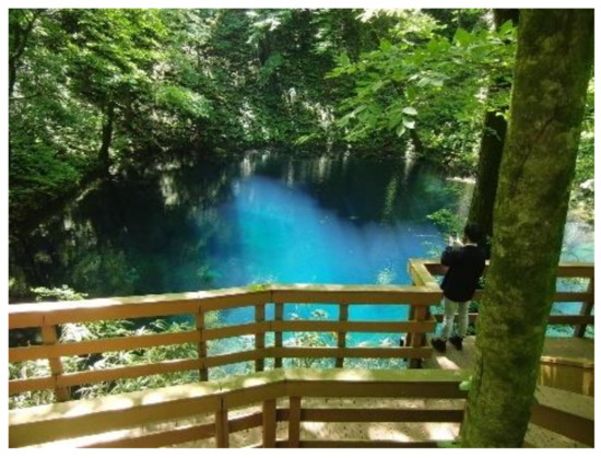
Figure 1.
Ao-ike Pond at 10:20 (JST), 5 June 2021.
Figure 2 shows the location of Ao-ike Pond and the surrounding pond group, called Juni-ko Lakes. Ao-ike Pond has three hydrological characteristics; it is the uppermost groundwater source to a series of ponds of the Koshiguchino-ike pond group (Figure 2), it has no inflowing and outflowing streams, and most of the pond water is supplied by spring water from the bottom [19]. At a viewpoint above the pond shore (Figure 1), under no wind, many springing ripples were seen on the water surface. Such ripples were also observed in spring at the water surface of the lower Ketobano-ike Pond neighboring the Ao-ike Pond (Figure 2), which is caused by the spring of groundwater from Ao-ike Pond. Water temperature of Ao-ike Pond is almost constant at 10 °C or less, in the whole layer even in summer [19].
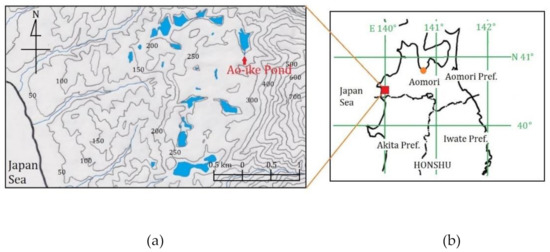
Figure 2.
Location of Ao-ike Pond and the surrounding pond group of Juni-ko Lakes in the northern Honshu Island (b) and on the topographic map (a) of 50 or 100 m interval (elevation in m above sea level).
How Juni-ko Lakes, including Ao-ike Pond, were formed is not yet clear [21]. Some geographers have been studying it. For example, by referring to results of the electrical resistivity tomography around Ao-ike Pond, Tsou et al. [22] suggested that the lake group was built up by a landslide of the large scale at a certain time.
Ao-ike Pond has a basin shape like a funnel, which was reported by Yoshimura et al. [20]. The present authors recognize that the shape is actually more like a quadrangular pyramid than a simple funnel type.
The water chemistry for Ao-ike Pond is already reported [21,23,24], but its details are omitted here. pH and electric conductivity at 25 °C (EC25) of the pond water were reported to be ca. 6.8 and ca. 20 mS/m, respectively, showing almost the same quantities as those of the downstream ponds [21].
There have been no coloring substances giving remarkable absorbances in the visible region of water color. The light absorption spectrum of the pond water in the visible region was reported to be same as that of pure water [25].
From early summer to autumn, especially in the afternoon on fine days, sunbeam trajectories can be observed in Ao-ike Pond from the observation deck. On the contrary, no sunbeam locus can be observed in spring.
Conceptual diagrams for occurrence of this phenomenon are displayed in Figure 3. In the Juni-ko Lakes area, deciduous broad-leaved trees dominate and the leaves of the trees tend to cover the surface of Ao-ike Pond from early summer to autumn. When the trees are growing leaves from early summer to autumn, it is considered that leaves above the water surface tend to shade solar radiation and light flux passing through the leaves make sunbeam trajectories inside the pond. On the other hand, most solar radiation is considered to enter the pond surface without shading in spring when the trees on the slope around the pond are leaf-free.
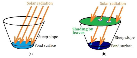
Figure 3.
(a) Situation surrounded by leaf-free trees on the slope. Most of solar radiation can then pass through the trees. (b) Situation surrounded by leaf-growing trees. The shading effect tends to produce a few sunbeams between the leaves.
The sunbeam trajectories include both contributions from scatterings inside the pond and reflection at the pond bottom at the different positions on the optical locus. The most important thing to pay attention to is that these contributions may separately be observed without any effects of the other light flux. The ordinary pictures of Ao-ike Pond suffered from the superposition of the lights by reflection and scatterings. Since observation and analyses of sunbeams can be expected to improve the accuracies, compared to conventional image analyses, this study proposes such an analytical method with high accuracy by actually analyzing sunbeams appeared in Ao-ike Pond images.
3. Formulation of the Coloration Model
In this section, the theoretical model by Hanaishi et al. [17] is reconstructed in terms of radiance.
3.1. Approximation of Pond Basin
As shown in Figure 4, the pond basin of Ao-ike Pond is approximated by a rotating paraboloid, according to what was mentioned in the previous section, with maximum depth d, pond surface radius r, horizontal distance from the pond shore to the observation point w, the height of the observation point h, and the clockwise angle η of the observation point direction from the west direction when viewed from the zenith. The coordinate of the observation point is written by H(−(r + w) sinη, −(r + w) cosη, h). The pond bottom point coordinate T1(x1, y1, z1) satisfies the following equations:
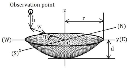
Figure 4.
Rotating paraboloid basin model for Ao-ike Pond.
3.2. Calculation of Observables Seen from the Observation Point by the Reverse Ray Tracing Method
3.2.1. Traveling Direction of the Light Flux
The light travels along the shortest path, obeying Fermat’s principle [12]. Hanaishi et al. [16] demonstrated that the optical path in consideration of refraction on the water surface can be calculated by solving a biquadratic equation, if the observation point and the irregular reflection point at the pond bottom or the scattering point inside the pond are given. On the other hand, Tadamura et al. [26] proposed a more sophisticated equation which concisely describes the refraction occurring at the horizontal interface, and a method for obtaining the optical path after a coordinate transformation.
Figure 5 shows the optical path diagrams in the case of irregular reflection on the pond bottom and scattering inside the pond.
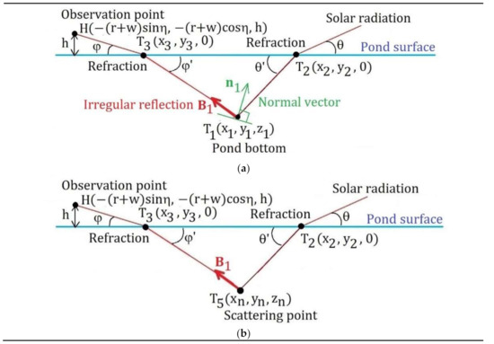
Figure 5.
Optical path diagrams in the case of (a) irregular reflection at the pond bottom and (b) scattering inside the pond.
3.2.2. Calculation of the Observable Quantities from Radiance
As shown in Figure 6, let L(x, ω) be the radiance of the light flux, emitted from the light source at the point x, where the reflection or scatterings occurs, in the direction of the solid angle ω.
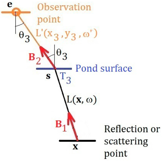
Figure 6.
Optical path of light flux above and below the pond surface.
Next, if this light flux is emitted from the pond surface at a certain point T3(x3, y3, 0) in the direction ω′, the radiance L′(x3, y3, ω′) is given by Equation (3) [1]:
where n12 is the relative refractive index of water with respect to atmosphere, and D (φ′, φ) is the Fresnel reflection and transmission coefficient [16] when the light flux is emitted from the pond surface.
Let us consider the observable quantity given by the next Equation (4), which expresses a differential light flux d2Ψ with the radiance of L′(x3, y3, ω′), an angle of θ3 between the direction B2 of the light flux and the vertical unit vector of k, a differential area of ds at the light emission point on the surface, and a differential solid angle of dω as shown in Figure 6:
This measurement problem was explained by Szirmay-Kalos [27]. Its conclusion is that the observable is obtained by multiplying the radiance by the scaling factor with the dimension of [radiance]−1, which is denoted by 1/B in this article.
Now, as shown in Figure 7, let e be the observation position, and s be the position of the point on the object. Let us consider an observation from this point e and look at the pixels on the window at position p. A solid angle Ωp is taken to be a small solid angle including the point s when viewed from the observation point e.
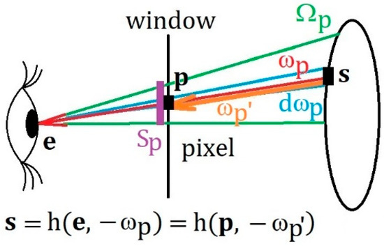
Figure 7.
Conceptual diagram of a point on the object, a point on the screen (pixel) on which they are viewed, and an observation position.
Now suppose that ωp is a solid angle that represents the direction in which the observation point e is viewed from s. Let ωp′ be a solid angle that expresses the direction in which the point p on the pixel is viewed from s. Sp is assumed to be the area of pixels on the window in the range of solid angle Ωp. Furthermore, we define y = h(x, −ω) as a visibility function indicating that the point y is in the direction of −ω from the point x. Hence, the point s on the object is expressed by s = h(e, −ωp) when viewed from the observation point e, and s = h(p, −ωp′) when viewed from the point p on the pixel. Likewise, let L(s, ω) be the radiance emitted from s in the direction ω.
The conclusion reached by Szirmay-Kalos [27] is that, from these definitions, the observable P is expressed by:
What is important in Equation (5) is that the distance from a point on the object to the observation point or its orientation has nothing to do with the observable.
This observation theory is now applied to the coloration of the pond surface. In the same way as was aforementioned, consider a light emission point T3(x3, y3, 0) on the pond surface. Let L′(x3, y3, ω′) be the radiance from here in the direction ω′. Assuming that this point is observable, in Equation (3), s = h(p, −ωp′) where s = (x3, y3, 0), thus the observable quantity of light from this point is given by:
Therefore, we have shown that the observable is the radiance multiplied by the scaling factor of 1/B.
Since the case of observation of the light flux from the emission point T3(x3, y3, 0) on the pond surface has been described so far, a method of extrapolating this to points other than the light emission point is described.
When the reverse ray tracing method is applied, reflection or scattering points are scanned and contributions from the corresponding area segments at the pond bottom or volume segments inside the pond, respectively, are superimposed as shown by Hanaishi et al. [17]. Here, the area segments are used in the case of irregular reflection at the bottom, and volume segments are used in the case of scattering in it.
The area segments of the pond bottom are taken to be parallel to the x and y axes, and the volume segments in the pond are rectangular parallelepipeds being parallel to the x, y, and z axes. These segments are obtained in grid patterns with Δx and Δy on the pond bottom or with Δx, Δy and Δz in the water body inside of the pond. Here, these increments Δx and Δy indicate the small lengths along x and y axes, respectively, when the area or volume segment is projected onto the horizontal plane. The parameter Δz expresses the vertical increment in volume segments and is introduced in the formulas for the light intensities of the scattered lights, as will be described later.
Hence, the division of the pond bottom or the water body into grids can be associated with multiplication of the observables by ΔxΔy and summing the quantities on each reflection or scattering point. In order to carry out the above summation, it is necessary to newly multiply the intensity formula by the factor with the dimension of [length]−2 from the viewpoint of the dimension.
On the other hand, it is assumed that this observable P′(x3, y3) gives P″(x, y) of the two-dimensional (2D) normal distribution centered on the light emission point T3(x3, y3, 0) and then is superimposed. The 2D normal distribution is assumed to take the form written in the following Equation (7) with multiplication by the 2D normal distribution density function (dimension: [length]−2) with the variance of σ2 (dimension: [length]2),
According to Equation (7), the observables have distributions on the pond surface. If the pond surface is assumed to be infinitely wide and the observables are integrated over the surface, then the integral is conservative. That is,
The sum of the above formula is expressed by:
where x3 and y3 are correlated to the area segment on the pond bottom or volume segment inside the pond, and these are taken at interval with Δx and Δy, respectively. When the segments are projected onto the pond surface, they give a spread of ΔxΔy at T3(x3, y3, 0).
Now, let us consider a simple example, as shown in Figure 8. What we examine next is that there should be no multiplication factor other than scaling factor of 1/B in the formulas for the observables.
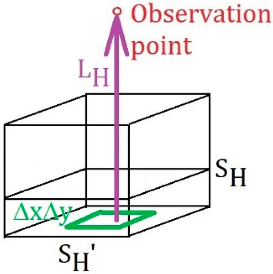
Figure 8.
Simple model for light emission.
It is assumed that the incident light enters a rectangular parallelepiped of a virtual pond from the zenith. Let SH′ be the bottom area of the rectangular parallelepiped. An irregular reflection point at the rectangle pond bottom or a scattering point at a rectangular parallelepiped in the pond with a thickness of one layer is assumed, and the pond bottom or scattering layer is gridded by Δx and Δy. Suppose that the light observed from the irregular reflection point or scattering point (xm, ym, zm) is generated. The formula which holds for the grid is as follows:
For the sake of simplicity, it is assumed that the irregularly reflected light or scattered light is observed from a sufficiently far point above the pond surface, and that these irregular reflection or scattering points provide a radiance LH of the uniform intensity from the area of SH′.
If the light intensity P′(x3, y3) ejected from the light emission point is distributed by a uniform 2D probability density of pH over the pond surface with the area of SH, then the light intensity distribution with the dimension of [length]−2 is expressed as follows:
Applying the idea of Equation (7),
In the rectangular parallelepiped we discuss now, the incident light enters from the zenith and the resulted lights are observed from directly above, so SH = SH′. Therefore, the following equation holds:
This means that the observable which is obtained by extrapolation from the emission points on the pond surface can be calculated from the radiance with simple multiplication by the scaling factor of 1/B. In the above simple case, we have taken a uniform probability density of pH = 1/SH, and have obtained the formula for the extrapolated observable. This consideration shows that we can express the extrapolated light intensity observables from the radiances belonging to the grids using the probability distribution function with the dimension of [length]−2. Thus, the density function for the 2D normal distribution will be one of the candidates owing to its dimension and normalization possibility.
Consequently, it is considered that the observable at any point on the pond surface can be calculated by extrapolation by Equation (7).
3.2.3. Digital Camera Sensitivity Coefficient and Scaling Factor
The scaling factor 1/B has a dimension of [radiance]−1 in this study, although in Hanaishi et al. [17] this factor was discussed based on the irradiance. Here, usage of the gray standard paper and its Lambertian reflecting property enabled us to determine the sensitivity factor of the digital camera in terms of the radiance, whereas the property could not be taken into consideration in our previous physical model described in terms of irradiance.
Here, flux, radiance and irradiance are the radiometric terms, and corresponding photometric terms are luminous flux, luminance and illuminance, respectively.
Let the aperture of the digital camera at the time of shooting be f/XE, the ISO sensitivity be IE, and the exposure time be TE. If the linear RGB values obtained from the image are (R, G, B), the output value corresponding to the luminance is expressed by Equation (14) [17,28]:
where the linear RGB values (R, G, B) denoted by 255t0 are connected to sRGB values 255t1 by Equation (15):
In order to convert the above output value Yout to an output OE of equivalent luminance, we use the following relation:
Next, the illuminance at a certain position from the light source is assumed to be EE, and this light is assumed to be reflected by the gray standard paper at this position. If this standard paper has a Lambertian surface with the albedo of RE, the luminance LE of the reflected light is written by:
Under these conditions, the photograph of the gray standard paper will be taken.
On the other hand, for the standard conditions of the digital camera, we assume that the aperture of the digital camera is f/XS, the ISO sensitivity IS, and the exposure time TS. Since the output value of the digital camera should be settled as 118 in terms of sRGB [28], we obtain the standard linear output as OS = γ−1(118/255) = 0.225 by using inverse transformation of t0 = γ−1(t1) defined by Equation (15) using the relation t1 = 118/255.
Assuming that the incident light flux from the source is apparently regarded as a parallel light and its illuminance is Es, the standard output value LS in terms luminance is expressed by LS = ES/π.
Therefore, the digital camera sensitivity coefficient β′1 is expressed by Equation (18) [28]:
The conversion factor F′S (dimension: [luminous flux]−1 [length]2 [solid angle] = [luminance]−1) from the luminance to the digital camera output is expressed by Equation (19):
When the intensity ratio of the actually observed image to the theoretically calculated one is settled to be β2, the scaling factor β‴0 (dimension: [luminance]−1) is given by Equation (20):
Assuming that the finally observed physical quantity is dimensionless and is normalized to 255, the scaling factor 1/B (dimension: [luminance]−1) can be described by the following formula:
where Km is a conversion factor from the radiometric quantities to the photometric ones, and Km = 683 lm/W.
3.3. Irregular Reflection
3.3.1. Lambertian Reflection Approximation of Irregular Reflection at the Pond Bottom
In the treatment which approximates the pond bottom to the Lambertian surface [12,14], the direction of incident light is represented by ωi, the direction of reflected light is ωo, the irradiance of incident light is E(ωi), the radiance of reflected light is L(ωo) and the reflection albedo is ρ. Then the radiance L(ωo) depends neither on ωi nor on ωo, and L(ωo) is expressed by Equation (22):
The Lambertian approximation is thought to be appropriate for pond bottoms consisted of sand or silt [12].
3.3.2. Consideration of Incident Angle of Light
Here, the effects of the incident angles of lights and of the slopes of the bottom at the irregular reflection points are considered.
As shown in Figure 9, if θ1 is the angle between the unit normal vector n1 = (n1x, n1y, n1z) at the pond bottom and the unit direction vector B1 along the traveling direction of the light flux in the pond after the irregular reflection, then the following equation holds:
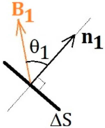
Figure 9.
Unit normal vector n1 at the pond bottom and unit direction vector B1 of the irregularly reflected light at the pond bottom.
3.3.3. Derivation of the Formula for Radiance
Consider an irregular reflection from an area segment located at the pond bottom point T1(x1, y1, z1) where the unit normal vector is n1. Now, we discuss the light intensity under the wavelength of λi.
Let L1 be the distance from the pond surface incident point T2(x2, y2, 0) to the pond bottom reflection point T1(x1, y1, z1), and L2 be the distance from the pond bottom reflection point to the pond surface emission point T3(x3, y3, 0).
We assume that the absorption coefficient of water is A(λi), density fluctuation scattering coefficient of water bw(λi), a white the Mie scattering coefficient of suspended solids bMie, phenomenological attenuation coefficient k1, the area segment ΔS with sides along the x and y axes at the pond bottom, and ΔxΔy is the normal projection of ΔS onto the horizontal plane.
For the pond bottom area segment ΔS, as shown in Figure 10, if the angle between the pond bottom unit normal vector n1 and the vertical unit vector k is θ2, then the normal projection of ΔS onto the horizontal plane becomes the increment ΔxΔy. Hence, ΔS is expressed as ΔxΔy divided by cosθ2, factor of the slope effect of the bottom. That is:
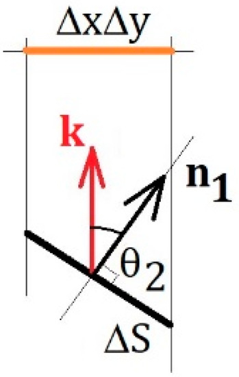
Figure 10.
Relationship between the area segment ΔS of the pond bottom reflection point and its projection ΔxΔy onto the horizontal plane.
Now, let PIrr′(x, y, λi) (dimension: [wavelength]−1) be the observable quantity of irregularly reflected light from the pond bottom. If the light intensity PIrr(θ, ϕ, x1, y1, z1, λi) (dimension: [wavelength]−1) corresponding to the irregular reflection point is expressed as follows, by taking the Fresnel reflection and transmission coefficient at the pond surface emission point as D(φ′,φ) [16]:
where the radiance LIrr (dimension: [light flux] [length]−2 [solid angle]−1 [wavelength]−1) in this equation is calculated next.
Let f(λi) be the spectral solar irradiance and D(θ, θ′) be the Fresnel reflection and transmission coefficient with the solar radiation incidence into the pond surface.
Using the solar irradiance f(λi) and a color matching function (λi), the illuminance in fine weather Efine can be obtained by Equation (27):
Assuming that the measured illuminance at the time of taking an image of the pond surface is Eobs, the effect of brightness of solar radiation can be incorporated with multiplication of the theoretical quantity by the factor Eobs/Efine.
If we assume that the multiplication factor of the incident light intensity, to which the slope of the pond bottom at the irregular reflection affects, is cosθ4, as shown in Figure 11, and that the vector A, with the opposite direction of the unit direction vector A″ of the incident light in the pond, satisfies A = −A″, then the following equation holds:
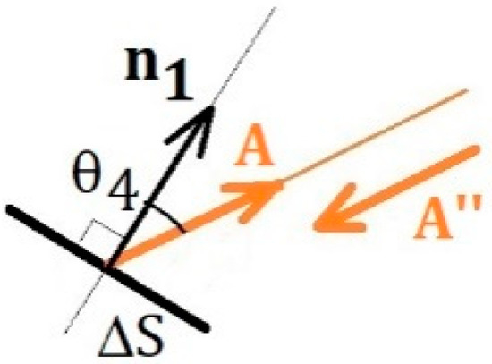
Figure 11.
Relationship between unit incident light vector A and unit normal vector n1.
Therefore,
where the unit incident light vector A can be expressed by Equation (30) from Hanaishi et al. [16] using the solar altitude θ and the azimuth angle ϕ. Here, the azimuth angle ϕ is taken in the direction of north (0) → east → south () → west → north when viewed from the zenith.
From the above consideration, the intensity P′Irr(x, y, λi) of reflected light from the pond bottom is expressed by Equation (31):
3.3.4. Calculation of the Observable
Wavelength integrations of the products of the intensity given by Equation (31) with the color matching functions are performed corresponding to each point on the pond surface, the tristimulus values XYZ are obtained, and the linear RGB values (non-dimension) are calculated by a linear transformation.
3.4. Density Fluctuation Scattering
Let L3 be the distance from the pond surface incident point T2(x2, y2, 0) to the scattering point T5(xn, yn, zn) inside the pond, and L4 be the distance from the scattering point to the pond surface emission point T3(x3, y3, 0).
The volume segment of the scattering point is parallel to the horizontal plane and the vertical direction, and the volume of this rectangular parallelepiped having sides of Δx, Δy and Δz along the x, y, and z axis directions, respectively, is ΔxΔyΔz.
In the same argument as was in pond bottom irregular reflection, the light intensity with the dimension of [wavelength]−1 is expressed for each scattering point as follows:
In the case of water density fluctuation scattering, if the phase function of scattering is (ΘS) and ΘS is the scattering angle, then the volume scattering function βw(λi, ΘS) is expressed by:
where the phase function is given by Morel et al. [29] as follows:
where δ1 is a depolarization factor.
As shown in Figure 12, the scattering angle ΘS is given by the following equation including the unit direction vector A″ of the light flux before scattering and the unit direction vector B1 of the light flux after scattering:
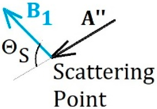
Figure 12.
Definition of scattering angle by two direction vectors before and after scattering.
Incident light on the volume segment at the scattering point is received in the horizontal plane of the segment. Its unit normal vector is equal to the vertical unit vector.
The effect caused by incident angle of light can be considered by analogy to the case where the light intensity of irregular reflection light is related to the incident angle as shown in Figure 11. We replace the unit normal vector n1 shown in Figure 11 with the vertical unit vector k, and we take A = (Ax, Ay, Az) as:
where
From the above considerations, the radiance LES emitted from the scattering point is written as follows:
.
Therefore, the light intensity P′ES(x, y, λi) of water density fluctuation scattered light is written by Equation (39).
In the same way as the pond bottom irregular reflection, the products of the intensity given by Equation (39) are taken with the color matching functions, integrated along the wavelength, and thus the tristimulus values are obtained, and these are linearly transformed to give the linear RGB values.
3.5. Mie Scattering
If the phase function of white Mie scattering with a scattering coefficient of bMie is (ΘS), then the volume scattering function βMie(ΘS) is written by:
As in the case of density fluctuation scattering, the equation giving the intensity P′Mie(x, y, λi) is as shown in Equation (41) via the following equation of the radiance emitted from the scattering point:
In the same way as the pond bottom irregular reflection and density fluctuation scattering inside the pond, the products of the intensity given by Equation (41) are taken with the color matching functions, integrated along wavelength, and then the tristimulus values are obtained, and these are linearly transformed to give linear RGB values.
4. Image Analyses
4.1. Image Analyses without Solar Shading by Tree Leaves above the Pond Surface
4.1.1. Image Data Used
Images were taken at four timepoints on 24 April 2021 when the weather was sunny and slightly cloudy without change during the shooting time. From the actual digital camera shooting conditions and the standard conditions (the digital camera aperture f/Xs = 2.8, ISO sensitivity IS = 100, exposure time TS = 1/100 s), the brightness within the actual images were standardized for analyses. The image data used are shown in Figure 13.
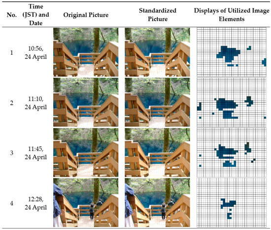
Figure 13.
Original pictures, standardized pictures, and displays of utilized color elements.
Ao-ike Pond images were taken with a digital camera of Panasonic DMC-LZ5. In order to obtain spectral reflectance of lights emitted from the pond, utilization of multi- or hyper-spectral camera is considered to be straightforward manner. However, in this study, the first goal was to theoretically reproduce the objective expressions of the pond colors that were photographed by a color camera. For the measurements of illuminances at the times of image captures, we used an illuminometer of Zhangzhou WeiHua Electronic LX-1010B near Ao-ike Pond, where no obstruction is in the sky. We corrected them by the solar altitudes to obtain the illuminances of solar radiations and utilized them in theoretical calculations.
In order to estimate the effect of shading over the pond surface, a fisheye lens was attached to a compact digital camera, and the hemispheres were photographed from the tip of the observation deck of Ao-ike Pond. These images were analyzed with a Gap Light Analyzer [30] to calculate the canopy openness. We used the Pentax Optio P70 compact digital camera, and the Gyorome No. 8 fisheye lens, purchased from FIT Co., Ltd. in Nagano, Japan. In this case, the portion of the image with a brightness equal to or higher than the threshold value was regarded as the sky. The contrasts of the photographs were lowered so that canopy openness was not overestimated.
4.1.2. Outline of Calculation Method of RGB Theoretical Values
As cited in Hanaishi et al. [16], the solar altitude θ and azimuth angle ϕ were calculated from the date and time, and the latitude and longitude of the observation site by Akasaka’s method.
The pond bottom irregular reflection points T1 or the scattering points T5 in the pond were scanned at intervals with Δx and Δy for the former cases and with Δx, Δy and Δz for the latter cases. The light incident points on the pond surface were obtained from these coordinates and from the direction vector of the solar radiation, using the above angles, θ and ϕ of the solar radiation, by the method described in Hanaishi et al. [16].
Next, from the coordinates of observation point H and scanning points T1 or T5, the biquadratic equation of Hanaishi et al. [16] for a square of b1z of the unit direction vector B1, here B1 = (b1x, b1y, b1z), of the light flux in water after irregular reflection or scattering was numerically solved by the DKA method. Because b1z is a positive square root of the positive solution of the biquadratic equation, we could obtain it satisfying 0 < b1z < 1. From thus obtained b1z, b1x and b1y were determined according to Hanaishi et al. [16] and the paths of lights after the reflection or scattering were determined so as to give the pond surface emission points T3.
Then parameters such as the cosine of the angle related to the path were determined, and in the case of scattering, the scattering angles and phase function values were obtained.
The calculations of colors as RGB values from the model formulas are given below:
- (I)
- In the case of irregular reflection at the pond bottom:
- step 1. Loop: Scanning the lake bottom T1(x1, y1, z1) at the intervals of Δx and Δy;
- step 2. Determination of the light incident point T2(x2, y2, 0) on the pond surface and of the emission point T3(x3, y3, 0) from the surface to obtain L1 and L2 in Equation (31);
- step 3. Calculations of the other factors determining the light intensities.
- step 4. Determination of PIrr(θ, ϕ, x1, y1, z1, λi);
- step 5. Loop: Scanning of the pond surface (x, y);
- step 6. Calculation of P′Irr(x, y, λi);
- End of loop of step 5;
- End of loop of step 1;
- (II)
- In the case of water density fluctuation scattering or in the case of Mie scattering:
- step 1. Loop: Scanning the in-lake scattering point T5(xn, yn, zn) at the intervals of Δx, Δy and Δz;
- step 2. Determination of the light incident point T2(x2, y2, 0) on the pond surface and of the emission point T3(x3, y3, 0) from the surface to obtain L3 and L4 in Equations (39) and (41);
- step 3. Calculations of the other factors determining the light intensities, e.g., scattering angles included in the estimations of phase functions;
- step 4. Determination of PES(θ, ϕ, xn, yn, zn, λi) or PMie(θ, ϕ, xn, yn, zn, λi);
- step 5. Loop: Scanning of the pond surface (x, y);
- step 6. Calculation of P′ES(x, y, λi) or P′Mie(x, y, λi);
- End of loop of step 5;
- End of loop of step 1;
- (III)
- Calculation of RGB values:
- step 1. Calculation of tristimulus values XYZ by integrating along wavelength after taking the products of P′Irr(x, y, λi)+ P′ES(x, y, λi)+ P′Mie(x, y, λi) with color matching functions.
- step 2. Calculations of RGB values within the range [0, 1] from XYZ by linear transformation, then normalization to 255 to obtain linear RGB values within the range [0, 255].
- step 3. Calculations of sRGB values within the range [0, 255] for displaying the color.
4.1.3. Applied Parameters
The spectral intensity of solar radiation in fine weather was referred from Hanaishi et al. [16]. The illuminance in fine weather was determined as Efine = 1.13 × 10⁵ lx by Equation (27).
The absorption coefficients of water were referred from Pope et al. [31], the density fluctuation scattering coefficients of water and its phase function were adopted from Morel [29] and Morel et al. [3] and the depolarization ratio of water was employed from Zhang et al. [32] as δ1 = 0.039.
Many types of Mie scattering phase functions have been used [33], but the most typical Petzold phase function [34] was utilized in this study.
4.1.4. Determination of Sensitivity Factor of the Digital Camera
The sensitivity factor of the digital camera, by which images of Ao-ike Pond were taken, was determined. The gray standard paper, purchased from Shenzhen Neewer Technology Co., Ltd. (Shenzhen, China), with the albedo of RS = 0.18 was used.
The illuminance from the halogen bulb (Panasonic JD110V65W-NP/EW) was measured using the illuminance meter and the reflected light from the gray standard paper was photographed with the digital camera.
The illuminance at a certain position from the halogen bulb was EE = 747 lx. The digital camera output as sRGB values on a picture of the gray standard paper at this position was converted to linear RGB values (R, G, B) = (167, 149, 115) giving OE = 0.591 by Equations (14) and (15). The digital camera conditions at this time were XE = 2.8, IE = 100, and TE = 1/30 s. The standard conditions are XS = 2.8, IS = 100 TS = 1/100 s, and ES = 2000 lx. By substituting these into Equation (18), the digital camera sensitivity coefficient β′1 = 11.7 was obtained.
Likewise, from Equation (19), F′S = 3.53 × 10⁻⁴ m2/cd was determined.
4.1.5. White Balance Problem in Image Analyses
In order to solve this problem, Hanaishi et al. [17] performed a significant difference test on the slope in the plots of the actually measured GB values versus the theoretically estimated ones for three images that might have different settings.
However, as described in the above theory, image analyses were performed by using these images to estimate the model parameters. Hence, the effect of the white balance correction could not be excluded, if three images suffered from the same white balance corrections, by means of comparing the measured RGB values with the theoretical ones which were obtained by using the model parameters.
Therefore, no mutual comparison of the three RGB values was possible unless the white balance problem was essentially solved.
Now, let (R, G, B) be the linear RGB values which give coloration on the pond surface. When the white balance correction parameters were written in a matrix form and RGB values were listed in a vector form, the matrix was diagonal and the RGB elements were not mixed. White balance correction only strengthens or weakens the RGB elements. When the RGB values are the same, the color tone from white to gray to black is given. To obtain these colors, we used the white balance correction. An example of the conversion matrix with non-zero off-diagonal elements is a conversion of RGB values to tristimulus value XYZ, where the off-diagonal matrix elements mix the RGB values.
That is, assuming that the coefficient of white balance correction was (wR, wG, 1), the corrected linear RGB values (Ra, Ga, Ba) were given by the following equation:
In the Ao-ike Pond image in this study, the R value was small and it was difficult to estimate wR. Therefore, we set as wR = 1, and only wG was determined by the image analyses.
4.1.6. Spectral Characteristics of Albedo at the Pond Bottom
Although the pond bottom albedo should initially have spectral characteristics, the coefficient of the albedo of the G value with respect to the B value was settled by wIrr,G and thus the intensity coefficient of irregularly-reflected light from the pond bottom was expressed as follows.
If the linear RGB values derived from the irregularly reflected light from the pond bottom were (RIrr, GIrr, BIrr) and the linear RGB values after correction were (RIrr,a, GIrr,a, BIrr,a), then the intensity coefficient wIrr,G for the G value obeys the following equation:
4.1.7. Outline of the Image Analysis Method
According to the method of Hanaishi et al. [17] acquisitions of the pond surface coordinate values from the digital camera image pixel values were taken, and the pond surface coordinate values corresponding to the color elements (shown in Figure 13) to be analyzed were obtained from the Ao-ike Pond images. The conversion parameters are listed in Table 1.

By the method of Hanaishi et al. [17], the measured RGB values were compared with the theoretical ones belonging to the coordinates (x, y) on the 1 m × 1 m lattice on the pond surface, by proportionally dividing the coordinate values to obtain the theoretical RGB values on the same coordinates as those of measured ones.
The model parameters were scanned in the theoretical calculation, the coefficient β2 to be multiplied in the calculation was determined according to the method of Hanaishi et al. [17], and the model parameters were settled so as to minimize the residual sum of squares of differences between the measured GB values and the theoretical ones.
4.1.8. Results and Discussion of Image Analyses
The canopy openness on 24 April 2021, when the four images in Figure 13 were taken, was 28 % as shown in Figure 14. On the other hand, sunbeams were observed on 9 May 2021, 20 May, and 5 June and on these 3 days the canopy openness were from 14 to 19%. Therefore, it was considered that the influence of shielding over the pond surface was smaller on 24 April than on the later observation dates.
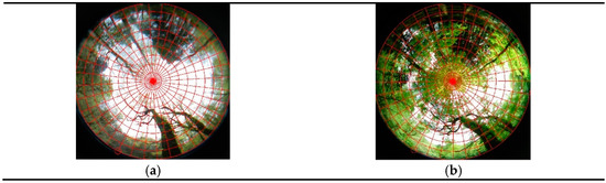
Figure 14.
Images of the sky above Ao-ike Pond taken with the fisheye lens. The grid is cut in 10° increment. (a) 24 April 2021 (b) 9 May 2021.
Table 2 shows the parameter set obtained by image analyses. Figure 15 depicts the simulation results of the Ao-ike Pond image, shown in Figure 13, at 12:28 (JST) of 24 April 2021. In addition, Figure 16 displays the fitting results. In these graphs, we show plots of theoretically predicted RGB values versus observed ones. The observed RGB values corresponded to the colors displayed in the column “Displays of utilized image elements” in Figure 13. The plots on RGB elements are shown on the same scales without any partial expansions, since determination of the model parameters were obtained by minimization of the residual sum of squares of differences between observed and theoretical GB values without weighting on G and B values.
Table 2.
Given and settled parameters in image analyses when the influence of shading over the pond surface by leaves was small.
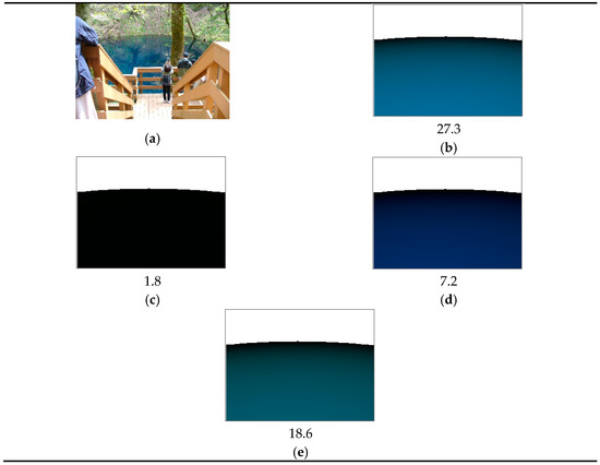
Figure 15.
Simulation results for Ao-ike Pond image; (a) Image taken at 12:28 (JST) of 24 April 2021, standardized by digital camera sensitivity, (b) sum of contributions from pond bottom irregular reflection, density fluctuation scattering by water and white Mie scattering, (c) contribution from pond bottom irregular reflection only, (d) contribution from density fluctuation scattering by water only, (e) contribution form Mie scattering only. The numerical values in (b–e) indicate relative averaged luminance on the pond surface.
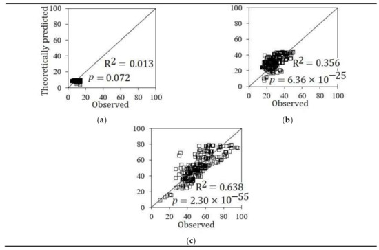
Figure 16.
Relationship between observed and theoretical RGB values of the model fitting in image analyses (n = 245). (a) R values, (b) G values and (c) B values.
In the fitting, as shown in Figure 16, the theory reproduced the measured RGB values well.
The simulation results shown in Figure 15 show the intensity ratio of pond bottom irregular reflection: density fluctuation scattering by water: Mie scattering was 1: 4: 10, which was significantly different from the ratio reported by Hanaishi et al. [16,17], where the contribution of pond bottom irregular reflection was large. Therefore, the potent mechanisms that contributed to the coloration of Aoike Pond were concluded to be the density fluctuation scattering by water and the white Mie scattering by suspended solids, in this study.
Before and after these two types of scatterings, along the optical paths inside the pond, absorption by water of long-wavelength visible light, i.e., red light, should occur and thus blue light remains and causes the blue coloration. Coloration by this mechanism in essence generates the blue color of water.
In addition, for the case of Ao-ike Pond, there is significant contribution of density fluctuation scattering. In this mechanism, blue light scatters more strongly than green or red light by a nature of water. The coloration caused by this mechanism emphasizes blue and the water body tends to exhibit a deep blue color. An example of the density fluctuation scattering by water for Ao-ike Pond is shown in Figure 15d.
It should be noted that this deep blue color of Ao-ike Pond originates from both blue coloration by absorption of red light by water along the optical path before and after the scattering inside the pond and blue coloration by the wavelength-dependent scattered light by water.
If water bodies contain a colorless and certain amount of suspended solids, the weak coloration effects by density fluctuation scattering of water is usually overridden by Mie scattering colorations by suspended solids which yield blue colorations as results of light absorptions by water. Coloration by this mechanism tends to exhibit a mixture of blue and white in the case where suspended solids in the water body are colorless, as shown in Figure 15e.
In the case of Ao-ike Pond, due to a low concentration of suspended solids within highly transparent water body, it was concluded that the pond water gives the coloration by density fluctuation of water as well as that by Mie scattering of suspended solids. This blue coloration can be considered to occur from the nature of water.
In this study, we judged that, by introducing the observation device theory, the contribution of three coloration mechanisms could be examined more accurately than by the theories reported by Hanaishi et al. [16,17].
4.2. Sunbeam Analyses
4.2.1. Utilized Images
Sunbeams images were taken on 9 May and 5 June 2021. The weathers in these shooting times were fine.
4.2.2. Acquisition of Coordinates on the Pond Surface from Images and Data Preprocessing
In the same way as the Section 4.1.7, we determined the conversion parameters in order to obtain the (x, y) coordinates on the pond surface from the pixel coordinates. The images were used after standardizations of the shooting conditions in the digital camera.
As shown in Figure 17, the slope of the straight line kl of the locus was obtained from a number of coordinates on the trajectory (e.g., (X1, Y1) and (X2, Y2)) on the pond surface, giving tanζ = kl.
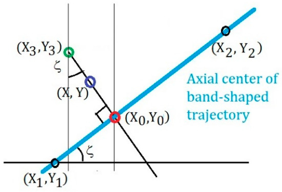
Figure 17.
Sunbeam coordinates on the pond surface images used to calculate the integrated data for image analyses.
The band width of the coordinates on lines perpendicular to the straight line of the optical locus was set to ±1 m, whose range included the number of points of 2Wl = 80. Thus, the 80 points on the perpendicular line were sampled as data from the pixels in the images.
To determine the pixel coordinate (Xp, Yp) corresponding to the point coordinate (X, Y) on the pond surface, we set a point on the axial center as (X0, Y0) and we used the following expressions where j was scanned from −Wl to Wl−1:
where the points (X3, Y3) in Figure 17 was defined by the following equation:
From the above (X, Y), the pixel values (Xp, Yp) on the image are obtained by the method of Hanaishi et al. [17].
Next, a band-shaped RGB data matrix was constructed as follows. In the longitudinal direction, matrix elements corresponded to (X0, Y0) along the optical locus of sunbeam on the pond surface were aligned. In the transverse direction, (X, Y), derived from (X0, Y0), along the perpendicular line to the axial center were aligned.
The band-shaped RGB data thus obtained might also include influences from fallen leaves on the pond surface. To avoid this effect, each pixel with the linear RGB values of R > 10 was excluded from the analyses.
Likewise, since the band-shaped RGB data matrix was denser than the original pixel data matrix, there were some matrix elements which the pixel data did not correspond to. In order to avoid the vacant elements in the band-shaped matrix, we carried out spline interpolations and then used the matrix of band-shaped RGB data with fully occupied elements.
From thus obtained band-shaped data (band width: 2Wl = 80), in order to obtain the integrated value along the axis perpendicular to the axial center, ±10 point-ranges, i.e., range with ±0.25 m from the center, were used. The increment of the distance Δl = 10/Wl2 × 1 m was multiplied and the sum was taken to obtain the integral along the transverse directions in the band-shaped RGB matrix. Figure 18 shows an example of the data (14:35 (JST) of 5 June 2021).
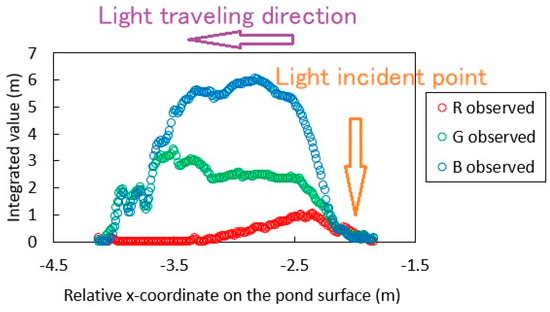
Figure 18.
Displays of integrated RGB data for image analyses. The x-coordinate on the horizontal axis was depicted in the relative coordinate system.
In Figure 18, the integrated RGB values are depicted for the x-coordinate on the pond surface in the relative coordinate system, i.e., the coordinate system seen from the observation point.
Likewise, in this figure, the range of sunbeam trajectory is −4.12 m < x <−1.83 m, and the data for image analyses were obtained by subtraction from the integrated RGB data by baselines obtained as the regression lines passing through the averaged values of RGB integrated data of 5 points just below x = −4.12 m and those of 10 points just above x = −1.83 m. The RGB integral values obtained from other sunbeam images were also subjected to the same processing, the base was subtracted and then analyzed.
In order to simulate the incidence of sunbeams into the pond, the reflection points at the pond bottom and scattering points inside the pond were scanned, with fixing the incident point of sunbeam of (x′K, y′K) in the absolute coordinate system obtained from the incident point of (xK, yK) in the relative coordinate system. We calculated the RGB values of sunbeam trajectories only when the incident point coordinates T2(x2, y2, 0) on the pond surface satisfied the following limitation expressions for optical paths with small Δa:
Next, the integral of the theoretical values along the perpendicular axis to the axial center were obtained by the following equation:
where (x3, y3) indicates the coordinates of the emission points of lights on the pond surface corresponding to the scanned reflection points at the bottom or scattering points inside the pond. Definitions of the RGB values, R(x3, y3) etc., are described below.
The above equations defined a one-dimensional distribution of integrated RGB values on an axial center of the light trajectory of the sunbeam. These equations were valid because of the following two reasons. The numerical calculations of the sunbeams were done under the optical path limitations, as described above. Here, the light emission point coordinates T3(x3, y3, 0) on the pond surface were located almost on a straight line along the axial center. In addition, the emission light intensities on the surface had the 2D point symmetrical distributions around T3(x3, y3, 0).
From Equations (31), (39) and (41), the following equations hold:
If we took the color matching functions as (λi), (λi), and (λi), the tristimulus values were:
Hence, RGB values were obtained by the following linear transformation described by Hanaishi et al. [16] as:
where, we defined as:
The dimensions of R(x3, y3), G(x3, y3) and B(x3, y3) were [length]2. Therefore, R(x0, y0), G(x0, y0) and B(x0, y0) had the dimension of [length], and the integral of the observed RGB values along one direction had the same dimension.
The parameters were determined so that the theoretical integrals obtained above would reproduce the integrated RGB values obtained from the observed RGB values.
4.2.3. Fitting of RGB Values Observed on the Pond Surface by the Formulation in this Study
Figure 19 shows the original images including the sunbeams, and their simulation results using the parameters obtained by the image analyses, and it demonstrates the appropriateness of fitting of the integrated value obtained from the observed RGB values by the model parameters. Table 3 tabulates the given and settled parameters for the model. The simulated sunbeam trajectory images in Figure 19 depict the observable quantities multiplied by 10 (β2 multiplied by 10).
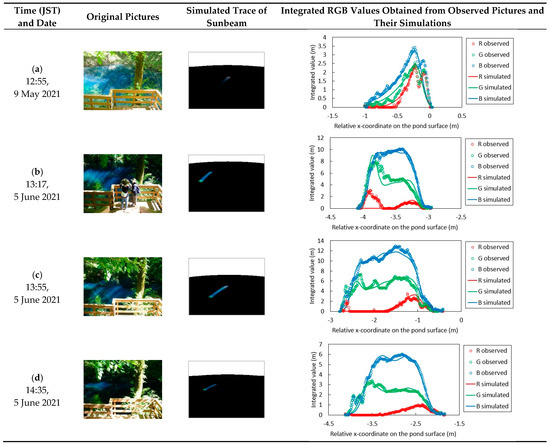
Figure 19.
Original images on (a) 9 May and (b–d) 5 June 2021, their simulations and integrated RGB values analyzed on sunbeams, which depict the situations for fitting.
Table 3.
Given and settled parameters applied in the image analyses. (a–d) correspond to the numbers in Figure 19. Common values of the parameters are listed below the table.
In addition, although the pond basin of Ao-ike Pond was approximated by the rotating paraboloid in this study, the coordinates of the pond bottom points where the incident sunbeams reached, were determined by the image analyses as the deviation from the approximated bottom coordinates as a rotating paraboloid, and the actual pond bottom points were obtained. The actual bottom depth parameters were expressed as kdd instead of d by using the parameter kd, and then the coloration calculations for sunbeam trajectories were performed.
4.2.4. Discussion
Sunbeams are rays of solar radiation passing through the gaps between the tree leaves incident into the pond. Since the effect of partial shielding by the leaves was considered to be less wavelength-dependent, we thought that the coloration theory reported by Hanaishi et al. [17] must be able to explain them.
However, the light trajectories reaching the pond bottom could not be reproduced by means of the previous coloration model [17], although the model [17] seemed to succeed in reproducing the image of Ao-ike Pond in fine weather without the influence of shading above the pond surface. The sunbeams images turned out to be possible to be reproduced with the new coloration model in this study.
The albedo ρ = 0.00027, as cited in Table 2, of the pond bottom irregular reflection obtained from the analyses of images with little influence of shielding above the pond surface had the same order of magnitude with 0.0003 ≤ ≤ 0.0005, cited in Table 3, as obtained from the sunbeam analyses, indicating that the physical model in this study could consistently estimate the parameters within two types of the images.
The correction coefficients in the white balance had the range of 0.85 ≤ wG ≤ 1.2. This suggested that the digital camera utilized in this study had almost the same white balance coefficient as the analyzed images.
Furthermore, the G/B correction ratio of the pond bottom albedos of the irregular reflections in the sunbeam analyses was in the range of 3 ≤ ≤ 4.
The Mie scattering coefficient was bMie = 0.05 m−1, as cited in Table 2, obtained by the image analyses when the influence of shielding above the pond surface was small, and the sunbeam image analyses gave 0.005 m−1 ≤ ≤ 0.2 m−1, as cited in Table 3. The Mie scattering coefficient obtained by two types of images had almost an equal order of magnitude, giving the same results as was aforementioned in the case of albedos at the pond bottom.
The parameters for the pond bottom depth were 0.63 ≤ ≤ 0.88. Therefore, it was considered that in three target images, as cited in Figure 19b–d, the sunbeams reached the shallower bottom than those expected from the rotating paraboloid basin model with maximum depth d of 8.8 m.
The image in which the sunbeams were observed and RGB integral values displayed in Figure 19 showed different tendencies in case (a). Figure 19a was photographed on 9 May 2021, when it had rained until just before the shooting, and the coloration was presumably considered to suffer from some influence of rain. The analysis results showed that both the white Mie scattering coefficient bMie and the phenomenological attenuation coefficient k1 were calculated to be larger than in other cases. It is suggested that suspended solids in the pond water were presumably brought by outflows of soil and/or sand from the slope surrounding the pond during and/or after rain and that these coefficients should become higher when the pond water contained suspended solids with the larger concentrations.
In addition, in Figure 20a–c, each contribution of three coloration mechanisms is drawn by using the parameters obtained by the sunbeam analysis depicted in Figure 19d (14:35 (JST) of 5 June 2021). From these figures, it was shown that the blue colors of sunbeams were caused by the density fluctuation scattering of water and white Mie scattering by suspended solids. This analysis results show good agreement with the analysis results of image with little influence of shielding above the pond surface.
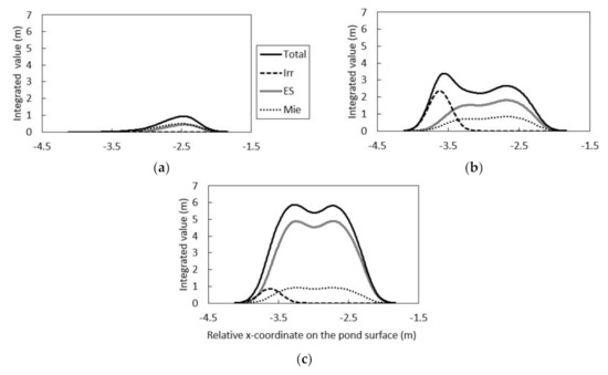
Figure 20.
(a) R value, (b) G value and (c) B value simulations for a sunbeam image (14:35 (JST) of 5 June 2021) as shown in Figure 19d, which are drawn separately for each contribution of pond bottom irregular reflection and in-pond scattering. The label “Total”: Pond bottom irregular reflection and in-pond scattering, “Irr”: Pond bottom irregular reflection only, “ES”: Water density fluctuation scattering only, “Mie”: Mie scattering contribution only. The graphs (a–c) are depicted in the relative coordinate system.
In the analyses of the sunbeams, the irregularly reflected lights from the pond bottom and the lights brought by scattering inside the pond could be analyzed separately along the optical locus.
As mentioned in the introduction, the coloration calculation of lakes can be made by the commercially available calculation software, but there are no other examples of theoretical reproductions of the light trajectories of sunbeams inside the pond passing through tree leaves. The authors think that the simulations of sunbeam trajectories described in this article belonged to the first case.
5. Conclusions
Formulas for quantitatively describing the coloration mechanisms of Ao-ike Pond were derived. Based on these formulas, three coloring mechanisms were anticipated; (i) pond bottom irregular reflection, (ii) density fluctuation scattering by water, and (iii) white Mie scattering due to suspended solids. In order to evaluate the physical model parameters, image analyses were carried out. The targets were RGB data of the images under little-shielded solar radiation onto the pond surface, and integrated RGB data from the optical path trajectories included in the sunbeam images. The following results were obtained:
- (1)
- The major causes producing the blue coloration of Ao-ike Pond are density fluctuation scattering by water and white Mie scattering by suspended solids for both the images with little-shielded solar radiation onto the pond surface and the sunbeam images.
- (2)
- In the calculations for the density fluctuation scattering of water, the pond coloration by the mechanism was calculated by applying the water absorption coefficient and the density fluctuation scattering coefficient of water, of which the values were cited in the previous literature. The coefficients were also obtained by other measurements, and this study can thus be the first case of theoretical reproduction of the digital camera images with blue colorations.
- (3)
- The analyses of the sunbeam image were performed by integrating the RGB values of the image along the axes perpendicular to the light trajectories and by theoretically reproducing the RGB values. Consequently, the RGB integral values were fairly well reproduced and the images with sunbeams were also well simulated. The theoretical reproduction of sunbeams onto the pond is considered to be the first instance as well.
In conclusion, regarding the coloration of Ao-ike Pond, the involvement of the coloration mechanism was clarified by analyzing two types of images, i.e., an image with little-shielded solar radiation over the pond surface and an image of sunbeams passed through the tree leaves above the pond.
By analyzing the sunbeam images, the contribution of irregular reflected light from the pond bottom and that of scattered light inside the pond were clearly separated, and thereby much information was obtained. Hence, the analytical method in this study is judged to be greatly useful for lake coloration studies in the future.
Author Contributions
Conceptualization, K.A.C. and R.H.; methodology, R.H.; software, R.H.; validation, K.A.C.; formal analysis, R.H.; investigation, K.A.C. and R.H.; resources, R.H.; data curation, R.H.; writing—original draft preparation, R.H.; writing—review and editing, K.A.C.; visualization, K.A.C. and R.H.; supervision, K.A.C.; project administration, K.A.C. All authors have read and agreed to the published version of the manuscript.
Funding
This research received no external funding.
Conflicts of Interest
The authors declare no conflict of interest.
References
- Jerlov, N.G. Marine Optics; Elsevier: Amsterdam, The Netherland, 1976. [Google Scholar]
- Kirk, J.T.O. Light and Photosynthesis in Aquatic Ecosystems, 3rd ed.; Cambridge University Press: Cambridge, UK, 2010. [Google Scholar]
- Morel, A.; Prieur, L. Analysis of variations in ocean color. Limnol. Oceanogr. 1977, 22, 709–713. [Google Scholar] [CrossRef]
- Smith, R.C.; Tyler, J.E. Optical Properties of Clear Natural Water. J. Opt. Soc. Am. 1967, 57, 589–595. [Google Scholar] [CrossRef]
- Smith, R.C.; Tyler, J.E.; Goldman, C.R. Optical Properties and Color of Lake Tahoe and Crater Lake. Limnol. Oceanogr. 1973, 18, 189–199. [Google Scholar] [CrossRef]
- Davies-Colley, R.J.; Vant, W.N.; Smith, D.G. Colour and Clarity of Natural Waters Science and Management of Optical Water Quality; The Blackburn Press: Caldwell, NJ, USA, 1993; pp. 17–19. [Google Scholar]
- Zhang, Y.; Giardino, C.; Li, L. Water Optics and Water Colour Remote Sensing. Remote. Sens. 2017, 9, 818. [Google Scholar] [CrossRef] [Green Version]
- Twardowski, M.; Tonizzo, A. Ocean Color Analytical Model Explicitly Dependent on the Volume Scattering Function. Appl. Sci. 2018, 8, 2684. [Google Scholar] [CrossRef] [Green Version]
- Zaneveld, J.R.V. An asymptotic closure theory for irradiance in the sea and its inversion to obtain the inherent optical properties. Limnol. Oceanogr. 1989, 34, 1442–1452. [Google Scholar] [CrossRef] [Green Version]
- Zaneveld, J.R.V. A theoretical derivation of the dependence of the remotely sensed reflectance of the ocean on the inherent optical properties. J. Geophys. Res. 1995, 100, 13135–13142. [Google Scholar] [CrossRef] [Green Version]
- Zaneveld, J.R.V.; Barnard, A.H.; Boss, E. Theoretical derivation of the depth average of remotely sensed optical parameters. Opt. Expr. 2005, 13, 9052–9061. [Google Scholar] [CrossRef] [PubMed] [Green Version]
- Mobley, C.D. Light and Water: Radiative Transfer in Natural Waters; Academic Press: New York, NY, USA, 1994. [Google Scholar]
- HydroLight-Sequoia Scientific. Available online: https://www.sequoiasci.com/product/hydrolight/ (accessed on 11 July 2021).
- Hedley, J. A three-dimensional radiative transfer model for shallow water environments. Opt. Expr. 2008, 16, 21887–21902. [Google Scholar] [CrossRef]
- PlanarRad. Available online: http://www.planarrad.com/index.php?title=PlanarRad (accessed on 11 July 2021).
- Hanaishi, R.; Osaka, N.; Chikita, K. A study on the coloration of Aoike Pond, Aomori Prefecture: Image analyses and modeling (in Japanese). J. Jpn. Soc. Phys. Hydrol. 2019, 1, 3–23. [Google Scholar] [CrossRef]
- Hanaishi, R.; Osaka, N.; Chikita, K. A study on the coloration of Aoike Pond, Aomori Prefecture: Elaboration of the model (in Japanese). J. Jpn. Soc. Phys. Hydrol. 2020, 2, 25–45. [Google Scholar] [CrossRef]
- Mikami, H.; Ishizuka, S.; Satoh, M.; Kon, T.; Noro, Y.; Tsushima, K.; Sakazaki, S.; Hayakari, T.; Oyamada, K.; Takayanagi, K.; et al. Natural Lakes in Aomori Prefecture (I) (in Japanese). Bull. Aomori Pref. Inst. Pub. Health Environ. 1992, 3, 50–59. [Google Scholar]
- Yoshimura, S. Water Temperature and Transparency of the Tugaru Zyûniko Lake Group. (2) Limnological Studies of the Tugaru Zyûniko Lake Group. Part 2 (in Japanese). Geog. Rev. Jpn. 1935, 11, 437–454. [Google Scholar] [CrossRef]
- Yoshimura, S.; Kiba, K.; Obara, N.; Nagatu, I. Morphology of the Tugaru Zyûniko Lake Group (1), Limnological Studies of the Tugaru Zyûniko Lake Group (1) (in Japanese). Geog. Rev. Jpn. 1934, 10, 968–989. [Google Scholar] [CrossRef]
- Tsushima, Y.; Hino, S.; Ohtaka, A.; Saito, S. Chemical Compositions of Lake Waters in the Tsugaru-Juniko Lakes, Aomori Prefecture, Northern Japan (in Japanese). Jpn. J. Limnol. 1995, 56, 9–18. [Google Scholar] [CrossRef] [Green Version]
- Tsou, C.; Yamabe, K.; Higuchi, D.; Sasagawa, T.; Kiriu, T.; Numata, S.; Furukawa, H.; Odagiri, M.S. High-resolution electrical resistivity tomography to investigate the origin of the Tsugaru-Juniko Lakes: An example near the Ao-ike (in Japanese). J. Jpn. Landslide Soc. 2021, 58, 109–117. [Google Scholar] [CrossRef]
- Hanaishi, R.; Kudo, S.; Nozawa, N.; Sato, H. A study on coloration mechanism of Aoike Pond in the Juniko region (the 1st report) (in Japanese). Annu. Rep. Aomori Pref. Publ. Health Environ. Cent. 2016, 27, 36–52. [Google Scholar]
- Matsutani, Z.; Kokubo, S. Studies on the Constituents of the Water of Koikuchi Lake Group, belonging to Tsugaru Jyuniko, in Aomori Pref. Japan (in Japanese). Nippon Suisan Gakkaishi 1942, 11, 5–15. [Google Scholar] [CrossRef]
- Hanaishi, R.; Osaka, N.; Shibata, M.; Nozawa, N.; Sato, H. Coloration mechanism of Aoike Pond in Lake Juniko (3rd report): Analyses of photometric results (in Japanese). Annu. Rep. Aomori Pref. Publ. Health. Environ. Cent. 2017, 28, 56–62. [Google Scholar]
- Tadamura, K.; Nakamae, E. Simulation for Lighting Design in/above the Water (in Japanese). J. Illum. Engng. Inst. Jpn. 1995, 79, 385–391. [Google Scholar] [CrossRef] [Green Version]
- Szirmay-Kalos, L. Monte Carlo Methods in Global Illumination Photo-Realistic Rendering with Randomization; VDM Verlag Dr. Müller Aktiengesellschaft & Co. KG: Saarbrücken, Germany, 2008. [Google Scholar]
- CIPA—Cameras & Imaging Products Association: CIPA Standards. Available online: https://www.cipa.jp/std/documents/download_e.html?CIPA_DC-004-2020_E (accessed on 11 July 2021).
- Morel, A. Optical Properties of Pure Water and Pure Sea Water. In Optical Aspects of Oceanography; Jerlov, N.G., Nielsen, E.S., Eds.; Academic Press: New York, NY, USA, 1974; pp. 1–24. [Google Scholar]
- Gap Light Analyzer (GLA). Available online: https://www.caryinstitute.org/science/our-scientists/dr-charles-d-canham/gap-light-analyzer-gla (accessed on 11 July 2021).
- Pope, R.M.; Fry, E.S. Absorption spectrum (380-700 nm) of pure water. II. Integrating cavity measurements. Appl. Opt. 1997, 36, 8710–8723. [Google Scholar] [CrossRef] [PubMed]
- Zhang, X.; Hu, L. Estimating Scattering of Pure Water from Density Fluctuation of the Refractive Index. Opt. Expr. 2009, 17, 1671–1678. [Google Scholar] [CrossRef] [PubMed]
- Mobley, C.D.; Sundman, L.K.; Boss, E. Phase function effects on oceanic light fields. Appl. Opt. 2002, 41, 1035–1050. [Google Scholar] [CrossRef] [PubMed] [Green Version]
- Petzold, T.J. Volume scattering functions for selected ocean waters. In Light in the Sea; Tyler, J.E., Ed.; Dowden, Hutchinson & Ross: Stroudsburg, PA, USA, 1977; pp. 152–174. [Google Scholar]
Publisher’s Note: MDPI stays neutral with regard to jurisdictional claims in published maps and institutional affiliations. |
© 2021 by the authors. Licensee MDPI, Basel, Switzerland. This article is an open access article distributed under the terms and conditions of the Creative Commons Attribution (CC BY) license (https://creativecommons.org/licenses/by/4.0/).