Visual-Saliency-Based Abnormality Detection for MRI Brain Images—Alzheimer’s Disease Analysis

Abstract

In recent years, medical image analysis has played a vital role in detecting diseases in their early stages. Medical images are rapidly becoming available for various applications to solve human problems. Therefore, complex medical features are needed to develop a diagnostic system for physicians to provide better treatment. Traditional methods of abnormality detection suffer from misidentification of abnormal regions in the given data. Visual-saliency detection methods are used to locate abnormalities to improve the accuracy of the proposed work. This study explores the role of a visual saliency map in the classification of Alzheimer’s disease (AD). Bottom-up saliency corresponds to image features, whereas top-down saliency uses domain knowledge in magnetic resonance imaging (MRI) brain images. The novelty of the proposed method lies in the use of an elliptical local binary pattern descriptor for low-level MRI characterization. Ellipse-like topologies help to obtain feature information from different orientations. Extensively directional features at different orientations cover the micro patterns. The brain regions of the Alzheimer’s disease stages were classified from the saliency maps. Multiple-kernel learning (MKL) and simple and efficient MKL (SEMKL) were used to classify Alzheimer’s disease from normal controls. The proposed method used the OASIS dataset and experimental results were compared with eight state-of-the-art methods. The proposed visual saliency-based abnormality detection produces reliable results in terms of accuracy, sensitivity, specificity, and f-measure.

1. Introduction

Alzheimer’s disease (AD) is the most common cause of progressive dementia in older adults [1]. AD can present as mental disorder, memory loss, language problem, or unpredictable behaviors. It occurs due to the death of neurons in different parts of the brain, and then throughout all of the areas of the brain at the final stage of AD. Brain tissue shrinks significantly. This disease generally occurs in older patients at an average age of 65 years and varies from individual to individual [2]. AD is not yet curable. Disease severity can increase for ten years after the diagnosis. The causes and reasons for the disease are still unknown to the medical community. Current treatment methods help manage symptoms in patients with AD. However, no treatment is available to completely cure the disease even though several medicines have been approved and tested recently.

Worldwide, more than 44 million people suffer from AD. This number will increase to more than 76 million by 2030 [3]. To diagnose Alzheimer’s disease in its early stages, proper medical images need to be studied.

Positron emission tomography (PET) magnetic resonance imaging (MRI), structural magnetic resonance imaging (SMRI), functional MRI (fMRI), and diffusion tensor imaging can indicate the biomarkers for human neuroimaging data [4,5,6,7]. MRI is fully non-invasive and is available worldwide. The mini-mental state examination (MMSE) is conducted by physicians to determine the impairment of patients with Alzheimer’s disease [8]. However, as part of automatic detection, image-based analysis is needed to correctly classify the stages of AD. MRI images clearly show the soft tissues of the brain. The temporal and parietal lobes of the brain can be seen clearly visualized on MRI. Changes in these lobes result in cognitive impairments in humans. The physician’s diagnosis is fully based on visual observation of the MRI. Interpretation of the MRI may vary from person to person. Therefore, an automatic diagnosis system is needed to assist physicians in making correct decisions about the disease. Most studies on Alzheimer’s disease have used MRI images for analysis. In these four proposed methods, MRI images were used for Alzheimer’s disease analysis. Figure 1 shows MRI images of a healthy person and a person suffering from dementia.

Several classification methods for AD have recently been reported. Calhoun et al. and Guo et al. reviewed Alzheimer’s disease classification based on MRI data [9,10]. Joint regression and classification [11] and weighted multi-modality-based classification [12] are mainly used to classify the disease. Two sets of strategies were applied in the brain morphometric analysis. Voxel-based morphometry and deformation-based morphometry are the two approaches currently used by the research community. In addition, machine-learning methods are used for the classification of Alzheimer’s disease [13]. Support vector machine (SVM)-based Alzheimer’s disease classification is mainly used by researchers. In this method, the SVM extracts high-dimensional features from MRI data and builds classification models to classify the disease. However, it mainly relies on the manual outlining of brain structures [14].

Lattice-independent component analysis and dendritic computing classifiers are used to perform MRI image classification of Alzheimer’s patients and normal patients [15]. Binary classifiers and single-neuron lattice models are used to perform the classification [16]. Initially, the disease-related features in the brain images are extracted by voxel morphometry analysis, and then a manifold-based semi-supervised learning framework is used to classify the disease [17]. Gray-level histogram-based MRI classification are also performed to identify anatomical changes in the hippocampus and thalamus regions [18].

Recently, deep-learning-based methods have been developed in the areas of computer vision, image understanding, natural language processing, etc. Deep-learning methods have also been used in medical image analyses. Prior feature selection is not required, and the input data can be optimally inferred [19]. This is one of the significant differences between deep-learning-based methods and other state-of-the-art machine learning methods.

In addition, visual saliency-based methods have recently been used for the analysis and classification of Alzheimer’s disease. Visual saliency maps play a vital role in the fields of computer vision and cognitive science. Automatic image analysis methods were inspired by researchers because the visual perception of radiologists was utilized by the saliency map to extract relevant disease regions [20]. Many algorithms and methods have been developed for visual saliency detection. Important and unimportant regions are segregated to perform image compression [21], segmentation [22], etc. By incorporating visual saliency analysis, the overall performance of the system is high with respect to performance metrics [23]. Many neurodegenerative diseases have very challenging image patterns that are not captured by region of interest (ROI) calculations and are time-consuming. The discrimination between mild and severe AD is challenging in the automatic diagnosis process.

In general, AD analysis is carried out with respect to the two datasets, ADNI and OASIS. Many literature reviews have been conducted on MRI image analysis for both datasets. The proposed method used the OASIS dataset for the experimental investigation. Alzheimer’s disease classification methods depend on personal clinical and demographic data. Four categories were used to analyze the AD classification using the proposed method.

The proposed method highlights the importance of saliency maps in AD analysis. Initially, the input MRI images were preprocessed using a statistical parametric mapping tool. Multiscale decomposition was performed using a wavelet transform. Wavelet decomposition was performed to obtain the essential features for saliency-map generation. Bottom-up and top-down saliency maps were obtained to obtain the final saliency map. Bottom-up saliency depends on the image features of the MRI. It is computed using the edge, texture, and orientation characteristics of the MRI images. An elliptical local binary pattern descriptor was leveraged to find low-level orientation characteristics. Top-down saliency uses the domain knowledge of the input.

Simple multiple-kernel learning (MKL) and simple and efficient MKL(SEMKL) were utilized to classify Alzheimer’s disease and normal patients. The experimental results showed reliable results in the performance metrics of accuracy, sensitivity, specificity, and f-measure. The results were compared with eight state-of-the-art methods that used the OASIS dataset for experimental analysis. 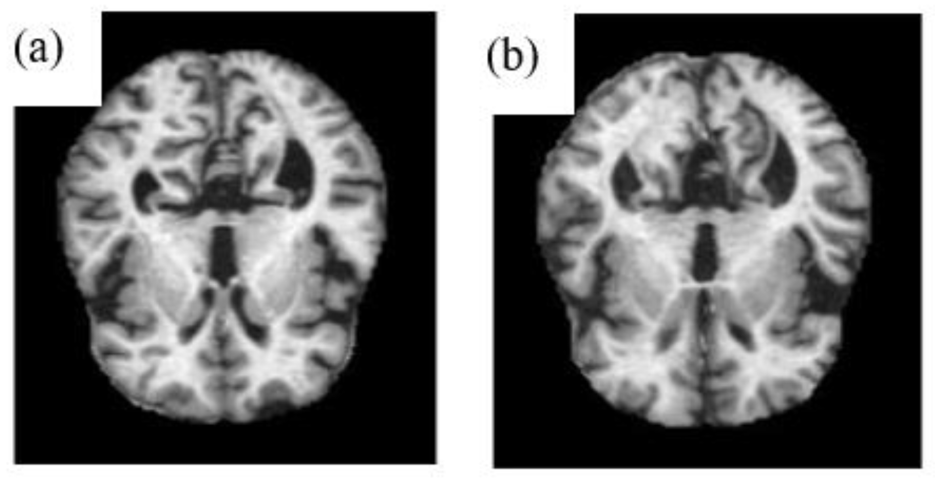The novelty of the proposed method lies in the use of an elliptical local binary pattern descriptor in the bottom-up saliency and usage of MKL and SEMKL for Alzheimer’s disease classification. Section 2 presents the proposed methodology, and this subsection presents the bottom-up and top-down saliency maps in detail. Section 3 presents the experimental results, performance metrics, and comparisons. Section 4 presents a discussion of the proposed method. The final section concludes the paper.

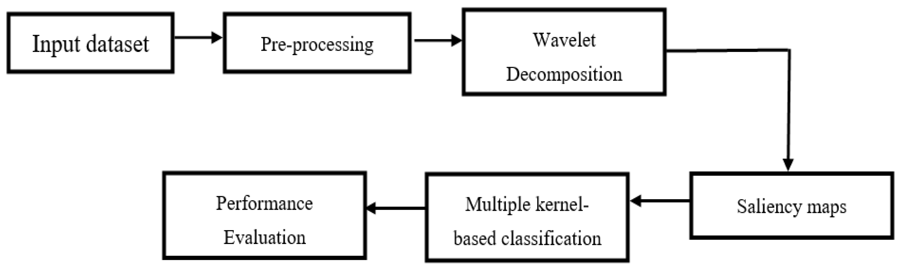
2. Proposed Methodology

A block diagram of the proposed method is shown in Figure 2. The major steps of the framework are wavelet decomposition, saliency map generation, and Alzheimer’s disease classification.

Figure 2 shows an overall block diagram of the proposed visual saliency-based Alzheimer’s disease classification. The proposed system framework consists of two important sections—saliency map generation and AD classification.

2.1. Pre-Processing

MRI images have different resolutions with respect to modern technology acquisition systems. In earlier days, MRI images had a pixel depth of 8. Currently, some image acquisition machines use a 16-bit form. To obtain a common platform, all images were scaled down to their 8-bit form. Therefore, the highest intensity value was taken as 1. The pre-processed image will help to obtain a correct classification and generate more accurate results. MRI images were pre-processed using SPM8. Statistical parametric mapping (SPM) is a tool that runs in MATLAB. It operates on a right-handed brain coordinate system. The T1-weighted structural images of each participant were automatically segmented into gray matter (g), white matter (m), and cerebrospinal fluid (c) by applying a mixture model cluster analysis. This ensures the construction of a spatially extended statistical process for inputs. Bias correction was not required during segmentation. After performing the normalization process, the MRI images were smoothed with a Gaussian filter that was applied through the VBM 8 toolbox [24].

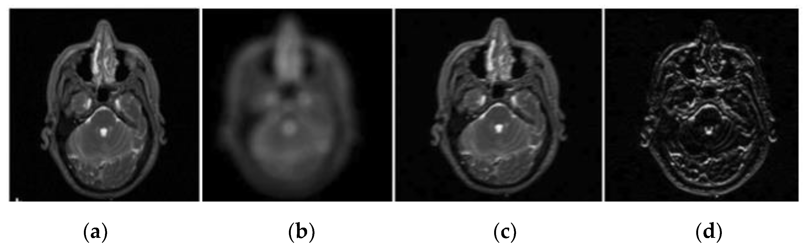
2.2. Wavelet Decomposition

Wavelet transforms are a powerful mathematical tool for image analysis. They provide simultaneous information about the image characteristics of frequency and time localization. Therefore, they are very helpful for classification tasks. Wavelet transformation produces results with less computation and no implementation complexity [25].

The input images $m\left(x,y\right)$ are decomposed into multiresolution sub-bands using a wavelet transform. The decomposed input images are represented as follows:

$$m\left(x,y\right)\to (m_{0}m\left(x,y\right),{\epsilon }_1\left(x,y\right),{\epsilon }_2\left(x,y\right),{\epsilon }_3\left(x,y\right)\dots \dots ..)$$

(1)

where $m_{0}m\left(x,y\right)$ is the low-frequency component approximation, and $\left({\epsilon }_1\left(x,y\right),{\epsilon }_2\left(x,y\right),{\epsilon }_3\left(x,y\right)\dots \dots ..\right)$ is the high-frequency component approximation. Unlike orthogonal cases, biorthogonal wavelet scaling functions are synthesizable. Biorthogonal wavelets were chosen with respect to the input MR images. They were also used to analyze the low-frequency images well. In the proposed method, a biorthogonal 9/7 wavelet filter was utilized for the decomposition. The MRI images were decomposed at different levels using wavelet analysis. A lower decomposition level provides less information, and a higher decomposition level provides more information to the classification unit. However, overfitting is a major concern when selecting the decomposition level. A five-level decomposition level was used in this method to prevent overfitting issues. The MRI axial view image obtained after wavelet decomposition is shown in Figure 3.

Wavelets divide the input images into different frequency components. The 3D volume of the MRI data is decomposed into multi-resolution sub-bands at different levels.

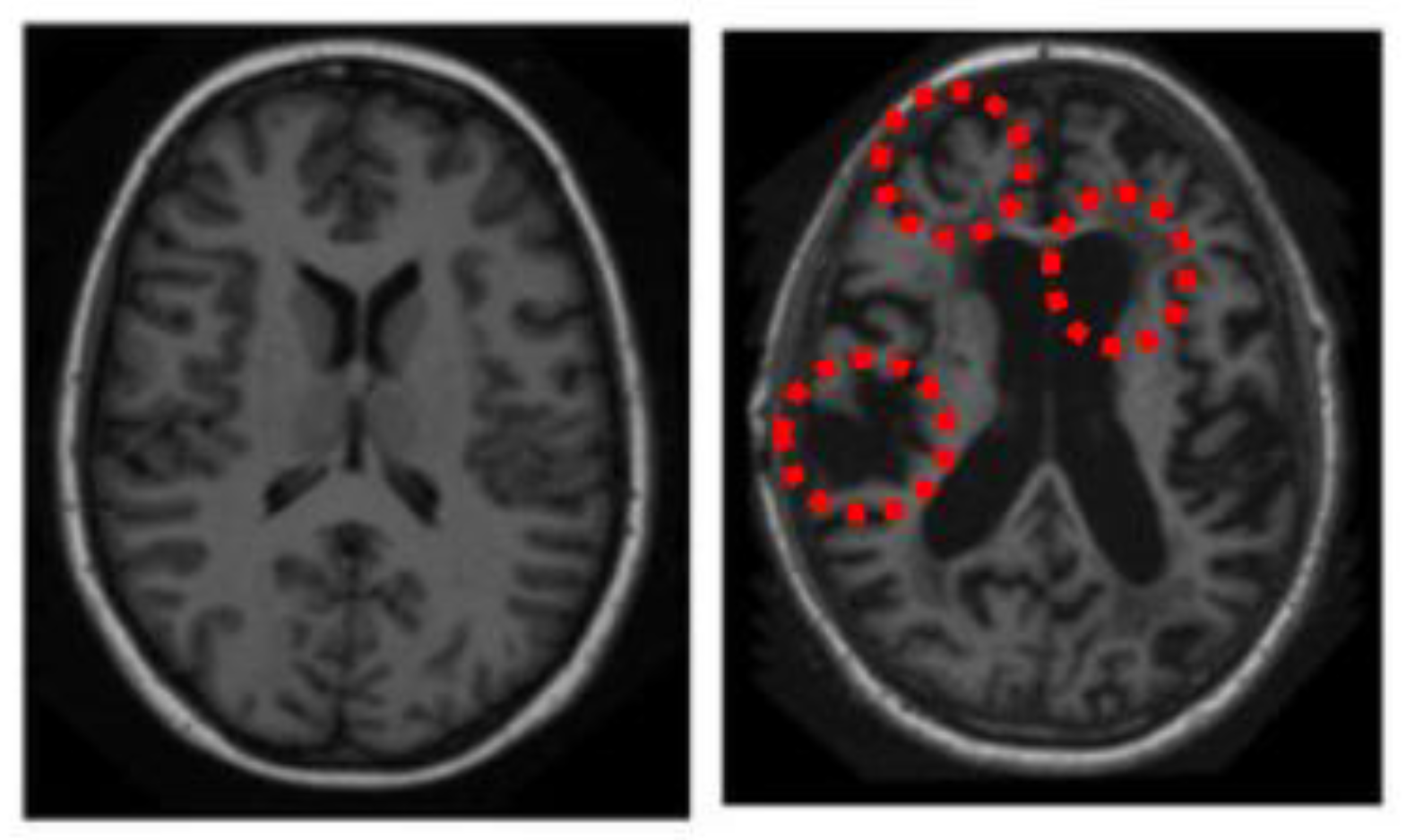
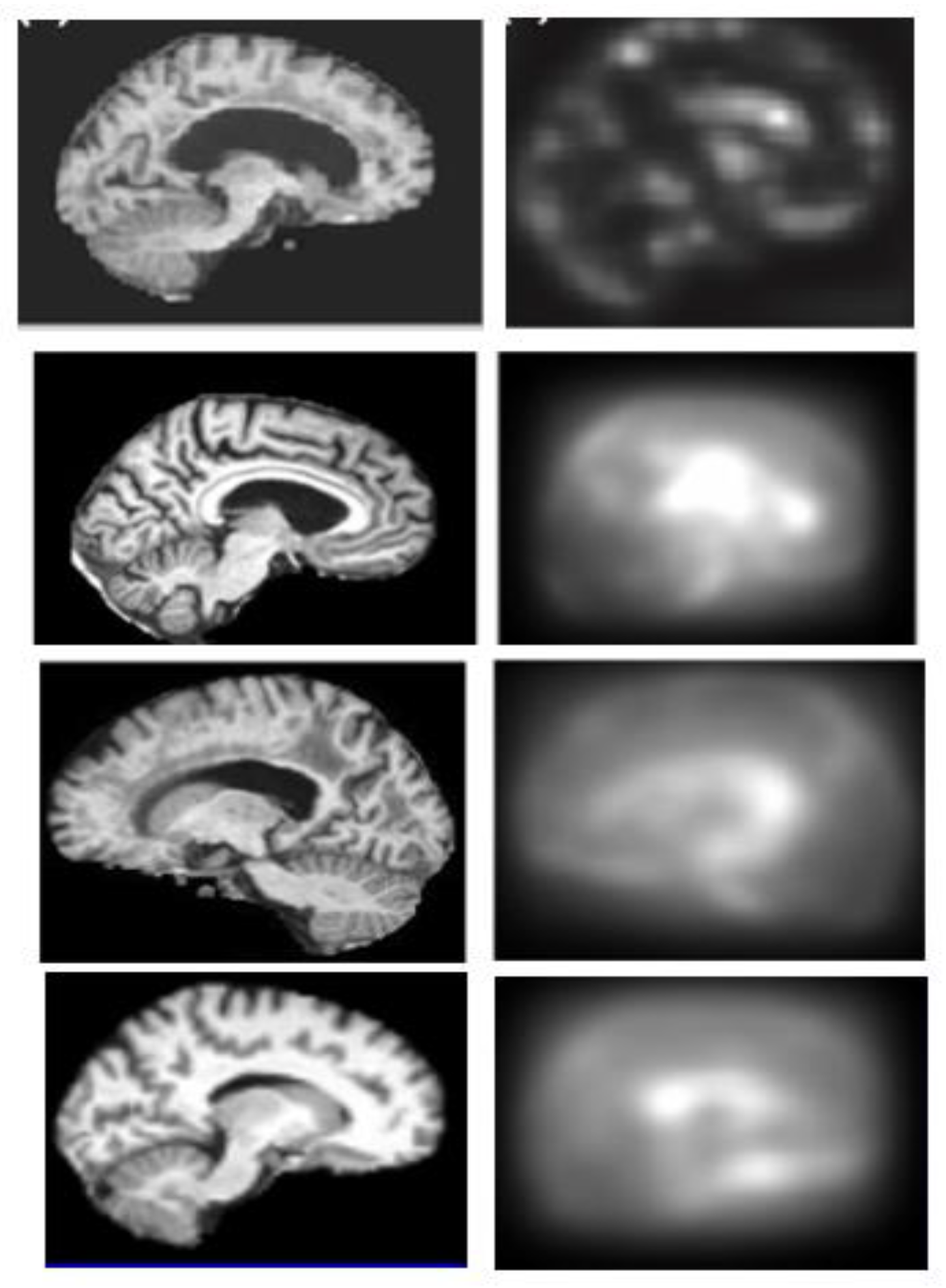
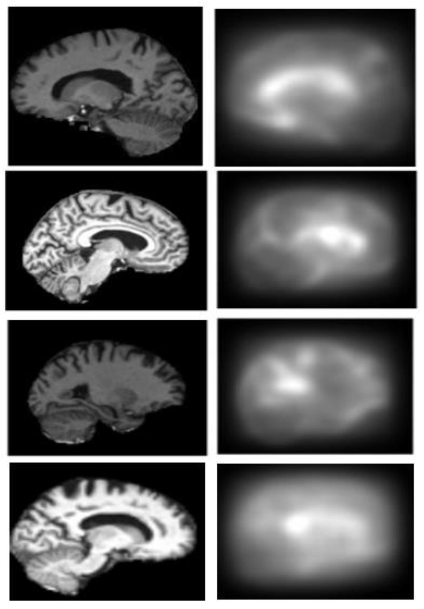
2.3. Generation of Saliency Maps

Visual saliency maps were generated from the input MRI images. In the proposed method, two saliency maps are combined to obtain the final saliency maps. The multi-scale analysis of the image characteristics was examined by the bottom-up phase. The low-level characteristics of input, such as intensity, orientation, and contrast, are considered for bottom-up saliency map construction. Top-down phases focus on high-level knowledge of the input. The properties of tissues are considered in the construction of the top-down saliency maps.

The extraction of feature maps from the input is the initial step in saliency computation. The intensity, orientation, and contrast are commonly used features for saliency calculations. Orientation filters like a Gabor resemble the visual cortex with respect to a particular field [20]. The corresponding feature maps were calculated at different scales.

The major steps which are involved in the saliency computations are as follows:

• Input: 3D MRI brain volume with $M=M_{ADP}+M_{NP}$
• $M_{ADP}$ is the Alzheimer’s disease pattern, $M_{NP}$ is the normal pattern.
• Step 1: Find the bottom-up and top-down saliency map;
• Step 2: Compute saliency map;
• Step 3: Classification of AD and non-AD interpretation.

2.3.1. Top-Down Saliency Maps ($S_T)$

In practice, a physician with some expertise can find the most atrophic brain areas in MRI images. According to neurodegeneration cell pattern, many brain areas are responsible for AD. Hence, the visual assessment of MRI images depends solely on brain shrinkage. This is accounted for in terms of tissue property variations.

In MRI analysis, brain deterioration is viewed as a variation of tissues in the gray matter or white matter. Tissue density variations in cell degeneration are the major differences between normal and Alzheimer’s disease brains. If cell density is reduced, it reflects the reduced volume in the structure of gray matter and white matter. This top-down knowledge was added to the saliency map. Loss of hippocampal volume differentiates the brain of a person suffering from Alzheimer’s disease from the brain of a normal person [26,27]. Normally, top-down saliency maps incorporate high-level knowledge denoted by brain MR volumes. Each MRI consisted of three tissues—gray matter, white matter, and cerebrospinal fluid.

To obtain the domain knowledge of each tissue, initially, a probability map was generated. A Gaussian distribution cluster analysis was used to segment the tissues. This was identified through the voxel intensity distribution of the brain tissue. This represents the distribution of tissues in the brain, which is calculated using a statistical parametric mapping approach. Probability map values range from 0 to 1. These maps highlight the spatial distribution of brain tissues. The intensity is proportional to the tissue volume before warping.

The probability map of a voxel at $\left(x,y\right)$ is $m_{0}m\left(x,y\right)$. It belongs to the $set=\left\{g,m,c\right\}$ and it is represented by $set=P\left(m\left(x,y\right)/set\right)$. If $P\left(m\left(x,y\right)/g\right)$ is the probability of a voxel being gray matter [28].

Steps for estimating the top-down saliency map ($S_T$)

• Build probability map;
• $m_{0}m\left(x,y\right)\leftarrow \mathrm{T}\left(m_{0}m\left(id\right)\right)for all id;$
• Regularize into a fixed range (0….1);
• If probability (g)> = 0.5 then
• $S_T\leftarrow m_{0}m\left(x,y\right)$
• else
• $S_T\leftarrow 0$;
• $end if S_T\leftarrow S_T\times \delta$.

Top-down saliency maps mostly depend on domain knowledge. According to the top-down saliency map construction steps, the saliency map is calculated by considering only visible voxels (the probability of gray matter being greater than 0.5). In the proposed method, top-down saliency was generated to identify whether the gray matter tissues of patients with AD varied from those of normal control patients. This is achieved through the rejection of irrelevant features from both cases. Min- max-margin discrimination is used to classify features between two classes, namely, the Alzheimer’s disease class and the normal control class [20]. It is an optimization task to classify each feature in the brain volume.

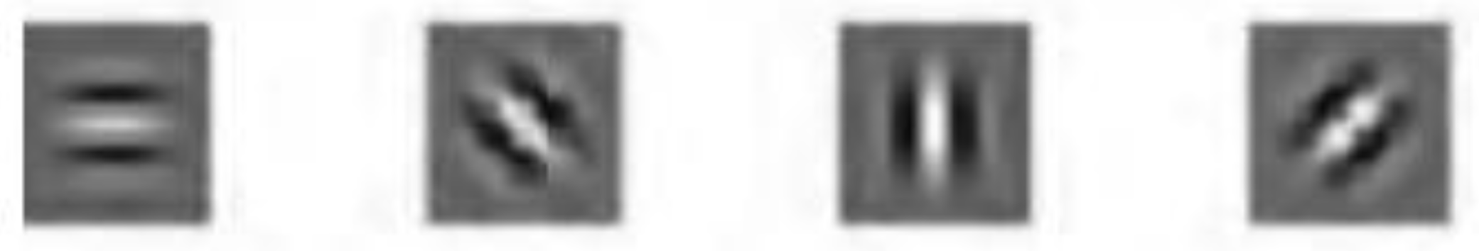
2.3.2. Bottom-Up Saliency Maps ($S_B)$

Bottom-up visual saliency maps rely on image features, such as color, edges, orientation, and textures. They mostly resemble the visual pattern of a physician. In this method, a bottom-up saliency map is derived from the cues of edges, orientation, and textures [28]. Edge cues are used to locate sudden changes in pixel intensity in MRI images, which portray discontinuities in white matter and gray matter tissues. Sobel and Canny edge detection are leveraged in the proposed method.

Elliptical Local Binary Pattern

An elliptical local binary pattern descriptor (E_LBPD) [29] was used to analyze the textural features of the MRI images. Ellipse-like topologies help obtain feature information from different orientations. To distinguish potential objects, a circular neighborhood was added to the texture descriptor. In elliptical local binary patterns, each center pixel (X_cp,Y_cp) and neighboring pixels (N) are located on an ellipse with radius distances r₁ and r₂. It is given by,

$$E_{LBPD}{}^{N,r_1,r_2}\left(X_{cp},Y_{cp}\right)={\displaystyle \sum }_{i=1}^{N}s\left(p_i{}^{N,r_1,r_2}-p_{cp}\right)2^{i-1}$$

(2)

where the ith neighboring pixel is (X_cp,Y_cp) is calculated as follows:

$$A_{step}=2·\raisebox{1ex}{$\pi $}\!\left/ \!\raisebox{-1ex}{$N$}\right.$$

(3)

$$x_i=x_{cp}+r_1·cos\left(\left(i-1\right)·A_{step}\right)$$

(4)

$$y_i=y_{cp}-r_2·sin(\left(i-1\right)·A_{step})$$

(5)

E_LBPD descriptors were used to extract more specific features from MRI images. They add additional directional features at different orientations that cover the micro patterns [29] where $p_{cp}$ is the gray level of the input image. This ensured that no pixels were omitted in accordance with the brain tissues. Gabor filters were utilized to highlight orientation features. These are linear filters. The orientation and frequency representations of Gabor filters are similar to those of humans. The real and imaginary components of the Gabor filter are given as:

$$G\left(x,y:\delta ,\theta ,\vartheta ,\tau ,\gamma \right)=e^{-\left(\frac{x^2+y^2{\gamma }^2}{2{\tau }^2}\right)}{e}^{i\left(\frac{2\pi x}{\delta }+\vartheta \right)}$$

(6)

where $\delta$ denotes the wavelength of the sinusoidal factor, $\theta$ represents the orientation of Gabor functions, $\vartheta$ represents phase offset, $\tau$ is the standard deviation of Gaussian envelope, and $\gamma$ represents the spatial aspect ratio.

The real and imaginary parts of the Gabor filter traveled in the orthogonal directions. Gabor filters with 0°, 45°, 90°, 135° orientations were considered to represent directional features. These features were obtained by convolving Gabor filters with different orientation angles with brain volume. Figure 4 shows the Gabor filter for different orientations in the MRI images. The edge, texture, and orientation features were obtained from multiple-scale MRI images and kept in separate feature maps. Finally, all feature maps were combined to obtain the final saliency map.

Bottom-up saliency maps are obtained by taking the geometric mean of the feature maps.

$$S_B=\frac{1}{2}(M{a}_{ed}+M{a}_{LBPD}+M_{GOrB})$$

(7)

where $M{a}_{ed}$—edge feature map, $M{a}_{LBPD}$—texture feature map, $M_{GOrB}$ is the orientation feature map.

2.3.3. Final Saliency Map

There are two different approaches to combining visual saliency maps. Max and average are the two methods used to perform feature integration. The max approach is used to identify regions that are salient in any of the components. The average method was used to obtain high saliency values for both components [30]. The final saliency map is a combination of the bottom-up and top-down saliency maps. The saliency map estimation provides details regarding the AD.

$$F{S}_{OV}=\sqrt{S_T{S}_B}$$

(8)

2.4. Multiple-Kernel Learning (MKL)

Multiple-kernel learning algorithms aim to discover the best combination of kernels to form the best classifier. Recently, different algorithms have been presented for forming two classes. The initial wrapper methods solve the MKL problem by handling a single SVM problem for a specific kernel weight. The second set of MKL algorithms uses optimization methods that reduce the number of computations. These methods use kernels that are larger than the wrapper methods. Basic multiple-kernel learning was discussed in [31] for simple classification problems. In the proposed method, a simple MKL and a simple and efficient MKL (SEMKL) [32] are used. The MKL method provides ordering for important features that are useful for classification tasks. Several studies have used MKL to classify genomic data and remote sensing data, and even though it is used for different classifications, it is an underestimated tool for Alzheimer’s disease analysis. This study aims to use the MKL methodology by highlighting its unique benefits.

The saliency maps contain information for classifying the AD and normal controls. Nevertheless, all parts do not have useful information for classification. Some regions have to be concentrated more for classification, whereas other regions are not highly concentrated. To analyze AD well, there is a mandate to reduce the size of the salient feature space. The Fisher discriminant ratio (FR) was used to characterize the classes. As it is a two-class classification problem, two means and two variances are obtained from the saliency map.

$$FR=\frac{{\left(m_1-m_2\right)}^2}{v_1{}^2+v_2{}^2}$$

(9)

where $m_i$ and $v_i{}^2$ are the mean and variance of the saliency maps, respectively. The FR value was calculated for each voxel of the volume. The FR value was taken as the threshold. If it is less than the threshold then more voxels can be selected. It also reduces the computational burden of voxel selection in the preliminary stage. It is used to select the most discriminative regions of the saliency map, which are used to segregate the disease images and normal control images. The classification performance was analyzed by varying the FR value.

The simple MKL uses a sub-gradient descent to fetch the direction that has the most improvement. Subsequently, a line search was used to catch the finest set of weights. The line search increases computational complexity; therefore, the SEMKL was used. The SEMKL dramatically decreases the number of computations by using a set of kernels derived from the Cauchy–Schwarz inequality. Prioritization of features and kernels is a prime consideration when choosing MKL algorithms. Kernel prioritization is important for overcoming the problems associated with MKL. The kernels can classify the data and provide boundaries [33].

The saliency maps provide a source of information on the location of the discriminative variations in the MRI images. They are the main source of differentiation between AD and normal diseases. In this method, multiple-kernel learning is used to classify the inputs [34]. The kernel matrices are of size M × M. A histogram intersection kernel is used to compute the similarity in the saliency maps. The kernel matrix is calculated between two saliency maps $SM,S{M}^{\prime }$.

$$KM\left(SM,S{M}^{\prime }\right)={\displaystyle \sum }_{i=1}^m\min \left(SM,S{M}^{\prime }\right)$$

(10)

The multiple-kernel methods have higher classification accuracies than single-kernel methods [33]. Simple MKL adopts a gradient descent on the support vector machine objective value and updates the kernel weights iteratively.

In addition, with multiple kernels, a single kernel was also calculated for each projection. All single kernels were summed using the weighted average method.

$$KM\left(SM,S{M}^{\prime }\right)={\displaystyle \sum }_{j=1}^3{w}_q{k}_q\left(SM,S{M}^{\prime }\right)$$

(11)

where $k_q$ is the histogram intersection kernel with ‘q’ projection and $w_q$ is the weight of the q projection. The decision parameter equation is given by Equation (12).

$$t\left(u\right)={\displaystyle \sum }_{i=1}^l{a}_{i}K\left(m,m_i\right)+b_i$$

(12)

where $a_i \mathrm{and} b_i$ are the coefficients that can be obtained from the input data. Multiple-kernel learning simultaneously determines the optimized coefficients for $a_i \mathrm{and}$ $w_q$.

Steps of MKL:

Step 1:

Initialize the range of kernels for MKL and SEMKL;

Step 2:

Compute the basic kernel matrixes using Equation (10);

Step 3:

Solve the projective direction according to Equation (11);

Step 4:

Using the projective direction ‘w’, combine the basic kernels;

Step 5:

Utilizing the combined kernel, the classification problem is approached via SVM.

The outcomes of the proposed classification results were compared with those of state-of-the-art methods. The results section emphasizes the experimental results using performance metrics.

3. Results

3.1. Dataset

The experiment was conducted using the Open Access Series of Imaging Studies (OASIS) dataset. The OASIS database consists of brain MRI images [35,36,37]. These image data were collected from MRI scans, diagnostic tests, and demographic data. Cross-sectional MRI and longitudinal MRI data are available in the OASIS dataset. MRI images were from 416 subjects between 18 and 96 years of age. The subjects were of both genders, and all were right-handed. A 1.5 T vision scanner was used to capture images from each subject. The MRI image acquisition details included the orientation of the sagittal plane and a flip angle of 10°. For this method, we randomly selected 200 subjects with complete demographic, clinical, or derived anatomic volume information [18]. One hundred patients were diagnosed with AD, and the other half were healthy subjects. The entropy-based sorting mechanism was used to obtain the most informative 32 images from the axial plane. Hence, 6400 images were used for training, of which 3200 images were AD and the other 3200 images were healthy. Figure 5 shows sample images from the OASIS dataset with AD and normal patient images. The red circles highlight the variations in AD images.

Table 1. Subject demographics and dementia status.

Condition	Numbers	Gender	Socioeconomic Status	Age		MMSE		CDR
				Range	Mean	Range	Mean	0	0.5	1	2
AD	100	M/F	2.94	66–96	78.08	15–30	24	0	31	17	1
Normal	100	M/F	2.88	65–94	77.77	26–30	28.96	49	0	0	0

provides additional information about the subjects.

All images were analyzed and diagnosed as AD and normal control images. The socio-economic status ranged from 1 (highest) to 5 (lowest). The Mini-Mental State Examination and Clinical Dementia Rating (CDR) were the medical parameters used to examine the images. MMSE scores ranged from 0 (worst) to 30 (best). All brain images consisted of 176 slices. Every single-slice MRI was represented by 176 × 208 pixels. Five categories of stages were taken by considering age group, clinical dementia rating (CDR), gender (F/M), and severity of disease. The CDR is a dementia staging factor that provides ratings to each subject.

Division 1:

Age 60–80, CDR=1, 7/6, 86 images, 20 D, 66 N;

Division 2:

Age 60–96, CDR=1, 7/6, 126 images, 28 D, 98 N;

Division 3:

Age 60–80, CDR= 0.5, 21/30, 136 images, 70 D, 66 N;

Division 4:

Age 90–96, CDR= {2,1,0.5}, 198 images, 100 D, 98 N.

where D is the Alzheimer’s disease image and N is the normal patient image. If the CDR is 0.5, the disease is very mild. If CDR is 1, then Alzheimer’s disease is mild and if CDR is 2, then Alzheimer’s disease is moderate.

AD classification performance depends on clinical and demographic data with respect to patients [33]. It is very difficult to discriminate between patients with very mild AD and those with normal conditions. Four categories were used to analyze the classification of AD. Figure 6 and Figure 7 also show such difficulties by viewing two types—Alzheimer’s disease patients and normal patients. In structural images, differentiating between the two types is difficult. The proposed method-based saliency maps exhibit slight variations, which can help in classification tasks.

3.2. Training and Testing

The parameter tuning of the proposed method is described in this section. The experimental investigations were carried out using MATLAB R2013, MathWorks, USA. A total of 75% of the input was used for training and 25% for testing. Cross-validation was used to determine the parameters that yielded the highest accuracy. Typically, the combination of kernels provides better results for classification tasks than a single kernel. The MKL is employed with cross-validation to identify which kernel is most suitable for classification, thereby producing good performance. Different k-fold scenarios (K = 3, 4, or 6) were adopted to select the training and testing data. Accuracy, sensitivity, and specificity were evaluated. The 6-fold cross-validation was performed to obtain better performance metrics.

3.3. Quantitative Analysis

In general, classification problems are evaluated using the performance metrics of accuracy, sensitivity, specificity, and F-measure. The proposed saliency-based, multiple-kernel learning classification is also quantified by the performance metrics of Accuracy (A), Sensitivity (S), Specificity (SP), and F-measure (Fm).

$$Accuracy \left(A\right)=\frac{\left(TP+TN\right)}{\left(TP+TN+FP+FN\right)}$$

(13)

$$Sensitivity \left(S\right)=\frac{\left(TP\right)}{\left(TP+FN\right)}$$

(14)

$$Specificity \left(SP\right)=\frac{\left(TP+TN\right)}{\left(TP+TN+FP+FN\right)}$$

(15)

$$F measure \left(Fm\right)=\frac{\left(2TP\right)}{\left(2TP+FN+FP\right)}$$

(16)

where $TP$ is true positive, $TN$ is true negative, $FP$ is false positive, and $FN$ is false negative.

Table 2. Performance metrics of the proposed approach.

	Accuracy (A)	Sensitivity (S)	Specificity (SP)	F-Measure (Fm)
Division 1	91.18	88.21	89.34	90.91
Division 2	88.26	86.15	87.33	87.81
Division 3	87.54	85.78	86.13	86.91
Division 4	84.23	82.91	83.21	84.12

presents the individual stage performance metrics.

From Table 2, it is ca be seen that the performance of elderly subjects decreased with mild Alzheimer’s disease. A comparative analysis was performed using state-of-the-art methods using the same OASIS dataset.

A comparative analysis was performed using the methods of Toews et al. [38], Andrea R et al. [39], Yang et al. [40], and Chyzhyk et al. [16,17]. The feature-based morphometry of Toews et al. [38], independent component analysis (ICA) of Yang et al. [40], and the support vector machine of Andrea et al. [39] were used in the comparative analysis. All of these methods use the OASIS dataset with four different groups. An equal error rate was used to classify diseases. ICA and SVM were used in [40]. In this method, the performance metrics are calculated using different formulae that are not in the standard definition formulae. The comparison method of Andrea et al. [39] used a saliency map and SVM for disease classification. The average error rate was 0.725, and the average accuracy was 74.54%. The proposed method is also compared with the recent literature involving with wavelet-transform-based feature detection. Jha et al. [41] used an extreme learning machine and dual-tree for concepts for AD classification. Zhang et al. [42] and Feng et al. [43] used wavelet entropy, particle swarm optimization, and neural network classifiers. The proposed method produced reliable results in the performance metrics of accuracy(A), sensitivity(S), specificity (SP), and F-measure (Fm).

The importance of the visual saliency map in AD classification is discussed and evaluated in the present study. Eight state-of-the-art methods for AD classification were used for the comparison. Visual saliency analysis and MKL were the most critical techniques adopted in the present study. The robustness of the proposed method is shown with respect to the performance metric scores.

4. Discussion

Computer-aided detection has attracted significant attention for brain image analysis. This is possible with advancements in machine learning and computational intelligence techniques. The proposed method deals with visual saliency-based Alzheimer’s disease analysis. This was accomplished using a saliency analysis of MRI images. Bottom-up and top-down information streams achieve the precise detection of AD and normal patients. Bottom-up saliency highlights the regions that are associated with AD diagnosis. This was obtained from different multiscale features. The major focus is on the construction of bottom-up saliency maps. An elliptical local binary pattern descriptor (ELBPD) was used to analyze the texture features of the MRI images. Ellipse-like topologies help to obtain feature information from different orientations. To distinguish potential objects, a circular neighborhood was added to the texture descriptor.

The top-down saliency map uses the domain knowledge of the MRI brain images. It adaptively chooses meaningful information. The entire saliency strategy allows the identification of structural regions that can be quantitatively related to AD detection. Information from the VBM is usually used for the statistical identification of different categories. The SPM8 tool was used to pre-process the MRI images. The pre-processed image will help to obtain a correct classification and generate more accurate results. The obtained saliency maps consisted of information for detecting AD and normal patients. None of the parts of the saliency map did not contain relevant information for detecting AD. To analyze AD well, the feature space size was reduced using the Fisher discriminant ratio. The MKL and SEMKL methods were adopted to discriminate between AD classes. MKL does not suffer from overfitting. The final decision was based on the weighted average of the SVM models. The kernel weights in MKL which are the most prominent in the classifier, were used to identify the data sources well.

The proposed study was conducted using the Open Access Series of Imaging Studies (OASIS) dataset. The present investigation involved extensive validation and parameter studies. Different factors are involved in bottom-up and top-down saliency, which are assessed based on the classification accuracy. This allows us to check the influence of different visual features and image scales on the final detection between AD and normal classes. The effective version of the proposed method attained an equivalent performance to that of state-of-the-art comparison methods in the

Table 3. Comparative analysis of proposed and state-of-the art methods.

Approach	Accuracy (A)	Sensitivity (S)	Specificity (SP)	F-Measure (Fm)
Toews et al. [38]	71.45	67.54	72.65	73.56
Yang et al. [40]	67.15	62.65	73.11	69.13
Chyzhyk et al. [16]	69	81	56	70.12
Chyzhyk et al. [17]	74.25	96	52.5	74.89
Andrea R et al. [39]	67.68	72	63.27	68.01
Feng J et al. [43]	86.4	82.11	89.91	--
Jha et al. [41]	78.48	75.35	79.98	--
Zhang et al. [42]	72.86	69.55	75.49	--
Proposed	89.12	86.71	87.31	88.93

. The comparison between the Chyzhyk et al. [16] method and the proposed method showed an average increment of 9.4% in accuracy and other performance metric calculations. Chyzhyk et al. [16] used dendritic computing to implement binary classifiers. Single-neuron lattice models were used to compute classification. With respect to performance metrics, the proposed method outperformed the methods of Yang et al. [40] and Andrea et al. [39]. The primary reason was the inclusion of elliptical local binary descriptors in the saliency map computations. The results of the proposed method were compared with eight state-of-the-art methods and produced 89.12% classification accuracy.

The proposed approach identifies the most relevant information for AD detection using saliency maps. These maps were derived from the orientation features, specifically at 0°, 45°, 90°, 135° and at different scales. The results show that the learning techniques used herein can separate the feature space that is related to AD and normal. The major contributions of this work include the use of an elliptical local binary pattern descriptor in the bottom-up saliency map computation and the use of MKL techniques in the classification. The major concern of many machine learning techniques is the overfitting problem. To address this issue, the proposed method uses MKL. It does not suffer from overfitting because the final decision is based on the weighted average of the SVM models. The state-of-the-art comparison methods have overfitting issues.

This study incorporated extensive validation and performance metrics. The input images were analyzed and experimented under different divisions. Many parameters were added to the top-down and bottom-up saliency. This information was assessed via classification accuracy. With an adequate and exhaustive evaluation, the present study can be effectively used to detect AD in normal patients. It identifies the influence of visual features on the final discrimination between normal and AD inputs. The major strengths of the present study are (i) the use of visual saliency analysis in AD detection, (ii) larger categories, (iii) rigorous validation using cross-validation, and (iv) comparable results. A limitation of the research is that subjects under 65 years of age were not included due to their high discrimination because this would be beyond the scope of this study and requires vast standardization procedures. The current work can be extended by improving the current system by using physician gaze tracking.

5. Conclusions

This study presents a computer-vision-based abnormality detection method for AD analysis. This demonstrates the importance of visual saliency in the classification of AD. Bottom-up and top-down saliency maps are derived from image features and domain knowledge. An elliptical local binary pattern descriptor was introduced to obtain low-level MRI characterization. This includes additional directional features at different orientations that cover the micro patterns. The proposed method applies MKL and SEMKL to classify AD from normal patients. The experiment was conducted using four categories of input from the OASIS dataset and achieved an accuracy of 89.12%. The results highlight a significant improvement compared to state-of-the-art methods. The proposed computer vision method can help physicians evaluate their diagnosis effectively and extract useful information quickly.

References

- Payan, A.; Montana, G. Predicting Alzheimer’s Disease: A Neuroimaging Study with 3D Convolutional Neural Networks. arXiv 2015, arXiv:1502.02506v1. [Google Scholar]
- Rossor, M.N.; Fox, N.; Mummery, C.J.; Schott, J.; Warren, J. The Diagnosis of Young-Onset Dementia. Lancet Neurol. 2010, 9, 793–806. [Google Scholar] [CrossRef] [Green Version]
- Sandanalakshmi, R.; Sardius, V. Selected Saliency Based Analysis for the Diagnosis of Alzheimer’s Disease Using Structural Magnetic Resonance Image. J. Med. Imaging Health Inform. 2016, 6, 177–184. [Google Scholar] [CrossRef]
- Marcus, C.; Mena, E.; Subramaniam, R.M. Brain PET in the Diagnosis of Alzheimer’s Disease. Clin. Nucl. Med. 2014, 39, e413–e426. [Google Scholar] [CrossRef] [PubMed] [Green Version]
- Lombardi, G.; Crescioli, G.; Cavedo, E.; Lucenteforte, E.; Casazza, G.; Bellatorre, A.G.; Lista, C.; Costantino, G.; Frisoni, G.; Virgili, G.; et al. Structural Magnetic Resonance Imaging for the Early Diagnosis of Dementia due to Alzheimer’s Disease in People with Mild Cognitive Impairment. Cochrane Database Syst. Rev. 2020, 3, CD009628. [Google Scholar] [CrossRef] [PubMed]
- Hojjati, S.H.; Ebrahimzadeh, A.; Babajani-Feremi, A. Identification of the Early stage of Alzheimer’s Disease Using Structural MRI and Resting-State fMRI. Front. Neurol. 2019, 10, 904. [Google Scholar] [CrossRef] [Green Version]
- Beheshti, I.; Demirel, H.; Farokhian, F.; Yang, C.; Matsuda, H. Structural MRI-based Detection of Alzheimer’s Disease Using Feature Ranking and Classification Error. Comput. Methods Programs Biomed. 2016, 137, 177–193. [Google Scholar] [CrossRef]
- Arevalo-Rodriguez, I.; Smailagic, N.; Figuls, M.R.I.; Ciapponi, A.; Sanchez-Perez, E.; Giannakou, A.; Pedraza, O.L.; Bonfill Cosp, X.; Cullum, S. Mini-Mental State Examination (MMSE) for the Detection of Alzheimer’s Disease and other Dementias in People with Mild Cognitive Impairment (MCI). Cochrane Database Syst. Rev. 2015, 2015, CD010783. [Google Scholar] [CrossRef]
- Calhoun, V.D.; Adali, T. Time-Varying Brain Connectivity in fMRI Data: Whole-brain Data-Driven Approaches for Capturing and Characterizing Dynamic States. IEEE Signal Process. Mag. 2016, 33, 52–66. [Google Scholar] [CrossRef]
- Guo, H.; Grajauskas, L.; Habash, B.; D’Arcy, R.C.; Song, X. Functional MRI Technologies in the Study of Medication Treatment Effect on Alzheimer’s Disease. Aging Med. 2018, 1, 75–95. [Google Scholar] [CrossRef] [Green Version]
- Zhu, X.; Suk, H.I.; Shen, D. A Novel Matrix-Similarity Based Loss Function for Joint Regression and Classification in AD Diagnosis. NeuroImage 2014, 100, 91–105. [Google Scholar] [CrossRef] [Green Version]
- Xu, L.; Wu, X.; Chen, K.; Yao, L. Multi-Modality Sparse Representation-Based Classification for Alzheimer’s Disease and Mild Cognitive Impairment. Comput. Methods Programs Biomed. 2015, 122, 182–190. [Google Scholar] [CrossRef]
- Liu, M.; Zhang, D.; Shen, D. Ensemble Sparse Classification of Alzheimer’s Disease. NeuroImage 2012, 60, 1106–1116. [Google Scholar] [CrossRef] [Green Version]
- Rathore, S.; Habes, M.; Iftikhar, M.A.; Shacklett, A.; Davatzikos, C. A Review on Neuroimaging-Based Classification Studies and Associated Feature Extraction Methods for Alzheimer’s Disease and Its Prodromal Stages. NeuroImage 2017, 155, 530–548. [Google Scholar] [CrossRef]
- Chyzhyk, D.; Graña, M. Optimal Hyperbox Shrinking in Dendritic Computing Applied to Alzheimer’s Disease Detection in MRI. In Proceedings of the Advances in Intelligent and Soft Computing, Salamanca, Spain, 6–8 April 2011; Volume 87, pp. 543–550. [Google Scholar]
- Chyzhyk, D.; Graña, M.; Savio, A.; Maiora, J. Hybrid Dendritic Computing with Kernel-LICA Applied to Alzheimer’s Disease Detection in MRI. Neurocomputing 2012, 75, 72–77. [Google Scholar] [CrossRef]
- Khajehnejad, M.; Saatlou, F.H.; Mohammadzade, H. Alzheimer’s Disease Early Diagnosis Using Manifold-Based Semi-Supervised Learning. Brain Sci. 2017, 7, 109. [Google Scholar] [CrossRef] [PubMed]
- Giraldo, D.L.; Garcia-Arteaga, J.D.; Cárdenas-Robledo, S.; Romero, E. Characterization of Brain Anatomical Patterns by Comparing Region Intensity Distributions: Applications to the Description of Alzheimer’s Disease. Brain Behav. 2018, 8, e00942. [Google Scholar] [CrossRef] [PubMed] [Green Version]
- Basaia, S.; Agosta, F.; Wagner, L.; Canu, E.; Magnani, G.; Santangelo, R.; Filippi, M. Automated Classification of Alzheimer’s Disease and Mild Cognitive Impairment Using a Single MRI and Deep Neural Networks. NeuroImage Clin. 2019, 21, 101645. [Google Scholar] [CrossRef] [PubMed]
- Rueda, A.; Gonzalez, F.A.; Romero, E. Extracting Salient Brain Patterns for Imaging-Based Classification of Neurodegenerative Diseases. IEEE Trans. Med. Imaging 2014, 33, 1262–1274. [Google Scholar] [CrossRef] [PubMed]
- Andrushia, A.D.; Thangarjan, R. Saliency-Based Image Compression Using Walsh–Hadamard Transform (WHT). In Biologically Rationalized Computing Techniques for Image Processing Applications; Lecture Notes in Computational Vision and Biomechanics; Hemanth, J., Balas, V.E., Eds.; Springer: Berlin/Heidelberg, Germany, 2018; Volume 25, pp. 21–42. [Google Scholar]
- Andrushia, D.; Thangarajan, R. Visual Attention-Based Leukocyte Image Segmentation Using Extreme Learning Machine. Int. J. Adv. Intell. Paradig. 2015, 7, 172. [Google Scholar] [CrossRef]
- Andrushia, A.D.; Thangarajan, R. An Efficient Visual Saliency Detection Model Based on Ripplet Transform. Sadhana 2017, 42, 671–685. [Google Scholar] [CrossRef] [Green Version]
- Wei, D.; Zhuang, K.; Ai, L.; Chen, Q.; Yang, W.; Liu, W.; Wang, K.; Sun, J.; Qiu, J. Structural and Functional Brain Scans from the Cross-Sectional Southwest University Adult Lifespan Dataset. Sci. Data 2018, 5, 1–10. [Google Scholar] [CrossRef] [Green Version]
- Ayadi, W.; Elhamzi, W.; Charfi, I.; Atri, M. A Hybrid Feature Extraction Approach for Brain MRI Classification Based on Bag-of-Words. Biomed. Signal Process. Control 2019, 48, 144–152. [Google Scholar] [CrossRef]
- Blennow, K.; Hampel, H.; Weiner, M.W.; Zetterberg, H. Cerebrospinal Fluid and Plasma Biomarkers in Alzheimer Disease. Nat. Rev. Neurol. 2010, 6, 131–144. [Google Scholar] [CrossRef] [PubMed]
- Braak, H.; Braak, E. Evolution of Neuronal Changes in the Course of Alzheimer’s Disease. J. Neural Transmission. Suppl. 1998, 53, 127–140. [Google Scholar] [CrossRef]
- Ben Ahmed, O.; Larabi, M.C.; Paccalin, M.; Fernandez-Maloigne, C. Saliency Guided Computer-aided Diagnosis for Neurodegenerative Dementia. In Proceedings of the 10th International Joint Conference on Biomedical Engineering Systems and Technologies, Porto, Portugal, 21–23 February 2017; pp. 140–147. [Google Scholar]
- George, M.; Zwiggelaar, R. Comparative Study on Local Binary Patterns for Mammographic Density and Risk Scoring. J. Imaging 2019, 5, 24. [Google Scholar] [CrossRef] [PubMed] [Green Version]
- Koutras, P.; Panagiotaropoulou, G.; Tsiami, A.; Maragos, P. Audio-Visual Temporal Saliency Modeling Validated by fMRI Data. In Proceedings of the 2018 IEEE/CVF Conference on Computer Vision and Pattern Recognition Workshops (CVPRW), Salt Lake City, UT, USA, 18–22 June 2018; pp. 2081–208110. [Google Scholar]
- Gevaert, C.M.; Persello, C.; Vosselman, G. Optimizing Multiple Kernel Learning for the Classification of UAV Data. Remote Sens. 2016, 8, 1025. [Google Scholar] [CrossRef] [Green Version]
- Xu, Z.; Jin, R.; Yang, H.; King, I.; Lyu, M.R. Simple and Efficient Multiple Kernel Learning by Group Lasso. In Proceedings of the 27th International Conference on Machine Learning (ICML-10), Haifa, Israel, 21–24 June 2010; pp. 1175–1182. [Google Scholar]
- Wilson, C.M.; Li, K.; Yu, X.; Kuan, P.F.; Wang, X. Multiple-Kernel Learning for Genomic Data Mining and Prediction. BMC Bioinform. 2019, 20, 426. [Google Scholar] [CrossRef] [Green Version]
- Ben-Ahmed, O.; Lecellier, F.; Paccalin, M.; Fernandez-Maloigne, C. Multi-View Visual Saliency-Based MRI Classification for Alzheimer’s Disease Diagnosis. In Proceedings of the 2017 Seventh International Conference on Image Processing Theory, Tools and Applications (IPTA), Montreal, QC, Canada, 28 November–1 December 2017; pp. 1–6. [Google Scholar]
- Rakotomamonjy, A.; Bach, F.R.; Canu, S.; Grandvalet, Y. SimpleMkl. J. Mach. Learn. Res. 2008, 9, 2491–2521. [Google Scholar]
- Marcus, D.S.; Wang, T.H.; Parker, J.; Csernansky, J.G.; Morris, J.C.; Buckner, R.L. Open Access Series of Imaging Studies (OASIS): Cross-sectional MRI Data in Young, Middle Aged, Nondemented, and Demented Older Adults. J. Cogn. Neurosci. 2007, 19, 1498–1507. [Google Scholar] [CrossRef] [Green Version]
- OASIS Brains—Open Access Series of Imaging Studies. Available online: https://www.oasis-brains.org (accessed on 15 July 2019).
- Toews, M.; Wells, W.; Collins, D.L.; Arbel, T. Feature-based morphometry: Discovering group-related anatomical patterns. NeuroImage 2010, 49, 2318–2327. [Google Scholar] [CrossRef] [PubMed] [Green Version]
- Andrea, R.; Fabio, A.G.; Eduardo, R. Saliency-Based Characterization of Group Differences for Magnetic Resonance Disease Classification. Dyna 2013, 80, 21–28. [Google Scholar]
- Yang, W.; Xia, H.; Xia, B.; Lui, L.M.; Huang, X. ICA-Based Feature Extraction and Automatic Classification of AD-Related MRI Data. In Proceedings of the 2010 Sixth International Conference on Natural Computation, Yantai, China, 10–12 August 2010; Volume 3, pp. 1261–1265. [Google Scholar]
- Jha, D.; Alam, S.; Pyun, J.Y.; Lee, K.H.; Kwon, G.R. Alzheimer’s Disease Detection Using Extreme Learning Machine, Complex Dual Tree Wavelet Principal Coefficients and Linear Discriminant Analysis. J. Med Imaging Health Inform. 2018, 8, 881–890. [Google Scholar] [CrossRef] [Green Version]
- Zhang, Y.; Wang, S.; Sui, Y.; Yang, M.; Bin Liu, B.; Cheng, H.; Sun, J.; Jia, W.; Phillips, P.; Gorriz, J.M. Multivariate Approach for Alzheimer’s Disease Detection Using Stationary Wavelet Entropy and Predator-Prey Particle Swarm Optimization. J. Alzheimer’s Dis. 2018, 65, 855–869. [Google Scholar] [CrossRef]
- Feng, J.; Zhang, S.W.; Chen, L. Alzheimer’s Disease Neuroimaging Initiative (ADNI). Identification of Alzheimer’s Disease Based on Wavelet Transformation Energy Feature of the Structural MRI Image and NN Classifier. Artif. Intell. Med. 2020, 108, 101940. [Google Scholar] [CrossRef]