Hysteresis-Based Current Control Approach by Means of the Theory of Switched Systems

Abstract

In this paper, a novel hysteresis-based current control approach is presented. The basis of the developed control approach is the theory of switched systems, in particular, the system class of switched systems with multiple equilibria. The proposed approach guarantees the convergence of the state trajectory into a region around a reference trajectory by selective switching between the individual subsystems. Here, the reference trajectory is allowed to be time varying, but lies within the state space spanned by the subsystem equilibria. Since already published approaches only show convergence to a common equilibrium of all subsystems, the extension to the mentioned state space is a significant novelty. Moreover, the approach is not limited to the number of state variables, nor to the number of subsystems. Thus, the applicability to a large number of systems is given. In the course of the paper, the theoretical basics of the approach are first explained by referring to a trivial example system. Then, it is shown how the theory can be applied to a practical application of a voltage source converter that is connected to a permanent-magnet synchronous motor. After deriving the limits of the presented control strategy, a simulation study confirms the applicability on the converter system. The paper closes with a detailed discussion about the given results.

1. Introduction

The climate crisis has brought the efficient use of resources more into the spotlight of society, politics, and science. Consequently, developers and manufacturers of electrical drive systems and electrical energy generation systems are more and more enforced to reduce resource consumption, both in production and in operation. Therefore, the system’s efficiency is also being increasingly used as a criterion for the controller design [1,2,3].

The classical separation of the current controller and the pulse width modulator into two subsequent components requires a precise design and synchronization [4]. On the other hand, the application of a hysteresis current control allows a combination of the system parts, and thus, a joint optimization. In addition, in [5], it was shown that a hysteresis current control is an effective way of achieving fast dynamic response. For this reason, the design and analysis of different hysteresis current controllers are the subject of many ongoing scientific works [5,6,7,8,9,10].

Due to the fixed sampling and switching instants of classical pulse width modulation (PWM) techniques, stability analyses of current control loops equipped with a PWM unit usually assume that the output voltage is sampled at the beginning of the PWM interval. This allows to deduce simplified, averaged PWM models, which reflect the small-signal behavior of the modulator [11]. However, the assumption of a constant output voltage is not always reasonable and represents a rather theoretical simplification, since the pulsed voltage causes significant but usually unmodeled current harmonics in many applications [12,13]. This is particularly relevant for small ratios between the PWM frequency and the angular frequency of the reference voltage. In addition, in the case of hysteresis-based controllers, no fixed sampling rate can be defined, but only an average period duration [7].

To overcome the limitations of the present modeling approaches, the theory of switched systems [14] can be applied. Following this theory, the use of averaged models can be avoided, as the system’s dynamical behavior in every switching state is inherently included in the model. Given a switched system, the Lyapunov theory is a proven tool for stability analysis [14,15,16,17]. Based on this theoretical background, refs. [18,19] analyzed the stability of switched systems with unique stable equilibria at every switching state, which can finally also be used to design hysteresis-based current controllers with guaranteed stability properties.

To demonstrate the basic ideas, this research focuses on an exemplary two-level converter system with inductive-resistive load and extends the general concept of [19] to a control law, which can also cope with time-varying reference trajectories. The paper is structured as follows. First, an introduction to the stability theory of switched systems is given; then, a hysteresis-based control is derived. Subsequently, the model of a voltage-source converter (VSC) plus load is introduced and the proposed control scheme is demonstrated by example. The paper concludes with simulations and a discussion of the results.

2. Theoretical Background and Proposed Control Law

2.1. General System Description of Switched Systems

In general, a switched system is described by

$$\begin{array}{cc}\hfill \dot{\underline{x}}\left(t\right)& ={\underline{f}}_{s\left(t\right)}\left(\underline{x}\left(t\right),\underline{u}\left(t\right)\right)\hfill \end{array}$$

(1)

where $\underline{x}\left(t\right)\in {\mathbb{R}}^n$ and $\underline{u}\left(t\right)\in {\mathbb{R}}^n$ are the state space and input vector, respectively. The function $s\left(t\right)$ represents a piece-wise defined switching sequence with values specified by the set of all different subsystems $\mathcal{S}=\left\{0,1,2\dots \right\}$. The time when $s\left(t\right)$ changes its value is named switching time or switching event.

The dynamic behavior of a switched system is determined, on the one hand, by the dynamics of the individual subsystems and, on the other hand, by the sequence of switching among these subsystems. There are many well-known methods to analyze the stability in the sense of Lyapunov of each subsystem [14,15,16,17,19]. However, even if all subsystems have the same stable equilibrium, it may be an unstable equilibrium of the switched system; see Figure 1. Moreover, on the contrary, a switched system might have a stable equilibrium, even if it is an unstable equilibrium for some or all subsystems; see Figure 2. In both cases, the switching sequence is responsible for the stability of the equilibrium.

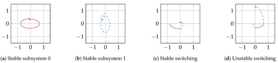
Figure 1. Switching between stable subsystems.

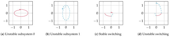
Figure 2. Switching between unstable subsystems.

The Lyapunov stability of switched systems was already discussed in literature and is a proven tool for stability analysis [14,15,16,17]. However, all methods require that the equilibria to be analyzed are in the origin, which forces the designer to perform a state transformation in advance. This process is usually even more difficult in practice, as it is often not desired to guarantee the convergence of the system trajectory $\underline{x}\left(t\right)$ to a constant equilibrium point, but rather to a subspace around a time-varying reference trajectory ${\underline{x}}_{\mathrm{ref}}\left(t\right)$. For example, this is also the case in converter applications.

In the following, this convergence is analyzed for linear switched systems of the form

$$\begin{array}{cc}\hfill \dot{\underline{x}}\left(t\right)& =\underline{\underline{A}}\left(\underline{x}\left(t\right)-{\underline{x}}_{\mathrm{eq},s}\right)+\underline{\underline{B}}\underline{u}\left(t\right),\hfill \end{array}$$

(2)

with unique stable equilibria ${\underline{x}}_{\mathrm{eq},s}$ for all $s\in \mathcal{S}=\left\{0,1,2\dots \right\}$. If, as in the case of switching converters, the plant’s input is known in advance, both the state trajectory $x\left(t\right)$ and the reference trajectory ${\underline{x}}_{\mathrm{ref}}\left(t\right)$ can be shifted by ${\underline{\underline{A}}}^{-1}\underline{\underline{B}}\underline{u}\left(t\right)$, i.e.,

$$\begin{array}{cc}\hfill \underline{\tilde{x}}\left(t\right)& =\underline{x}\left(t\right)+{\underline{\underline{A}}}^{-1}\underline{\underline{B}}\underline{u}\left(t\right),\hfill \end{array}$$

(3)

$$\begin{array}{cc}\hfill {\underline{\tilde{x}}}_{\mathrm{ref}}\left(t\right)& ={\underline{x}}_{\mathrm{ref}}\left(t\right)+{\underline{\underline{A}}}^{-1}\underline{\underline{B}}\underline{u}\left(t\right).\hfill \end{array}$$

(4)

Since both $\underline{x}\left(t\right)$ and ${\underline{x}}_{\mathrm{ref}}\left(t\right)$ are shifted by ${\underline{\underline{A}}}^{-1}\underline{\underline{B}}\underline{u}\left(t\right)$, the convergence of $\underline{\tilde{x}}\left(t\right)$ to a subspace ${\mathcal{R}}_{\delta }^n$ around ${\underline{\tilde{x}}}_{\mathrm{ref}}\left(t\right)$ deduces the convergence of $\underline{x}\left(t\right)$ to an equivalent subspace around ${\underline{x}}_{\mathrm{ref}}\left(t\right)$. The subspace ${\mathcal{R}}_{\delta }^n$ is bounded by the hysteresis threshold $\delta$ for the weighted distance between $\underline{\tilde{x}}\left(t\right)$ and ${\underline{\tilde{x}}}_{\mathrm{ref}}\left(t\right)$ and is defined by

$$\begin{array}{cc}\hfill {\mathcal{R}}_{\delta }^n& =\left\{{\mathbb{R}}^n\left|{\left(\underline{\tilde{x}}\left(t\right)-{\underline{\tilde{x}}}_{\mathrm{ref}}\left(t\right)\right)}^T\underline{\underline{M}}\left(\underline{\tilde{x}}\left(t\right)-{\underline{\tilde{x}}}_{\mathrm{ref}}\left(t\right)\right)<\delta \right.\right\}\hfill \end{array}$$

(5)

where the weighting matrix $\underline{\underline{M}}$ is positive definite. In summary, it can be supposed that there exists a switching control law that guarantees the convergence of the shifted state trajectory $\underline{\tilde{x}}\left(t\right)$ to ${\mathcal{R}}_{\delta }^n$, if:

• The state trajectory $\underline{x}\left(t\right)$ of the switched system in (2) converges to a unique stable equilibrium ${\underline{x}}_{\mathrm{eq},s}$ for each $s\in \mathcal{S}=\left\{0,1,2\dots \right\}$ if subsystem s is active and $\underline{u}\left(t\right)=0$.
• The input $\underline{u}\left(t\right)$ is continuous and given in advance;
• The shifted reference trajectory ${\underline{\tilde{x}}}_{\mathrm{ref}}\left(t\right)\in {\mathcal{R}}_{\mathrm{ref}}^n\subset {\mathbb{R}}^n$, where ${\mathcal{R}}_{\mathrm{ref}}^n$ is specified by the vector space, spanned by the subsystem equilibria ${\underline{x}}_{\mathrm{eq},s}$ for all $s\in \mathcal{S}$;
• The slowest mode of the system trajectory $\underline{x}\left(t\right)$ is faster than the fastest mode of the reference trajectory ${\underline{x}}_{\mathrm{ref}}\left(t\right)$.

To illustrate condition three, Figure 3 shows the equilibria of an exemplary switched system in ${\mathbb{R}}^2$ with three subsystems, $\mathcal{S}=\left\{0,1,2\right\}$, a shifted reference trajectory ${\underline{\tilde{x}}}_{\mathrm{ref}}\left(t\right)$, and the corresponding sets ${\mathcal{R}}_{\delta }^2,{\mathcal{R}}_{\mathrm{ref}}^2,{\mathbb{R}}^2$ for some $t_0>0$.

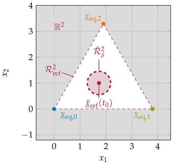
Figure 3. Shifted reference trajectory ${\underline{\tilde{x}}}_{\mathrm{ref}}\left(t_0\right)$ subspaces ${\mathcal{R}}_{\delta }^2$, ${\mathcal{R}}_{\mathrm{ref}}^2$, and subsystem equilibria ${\underline{x}}_{\mathrm{eq},0}$, ${\underline{x}}_{\mathrm{eq},1}$, and ${\underline{x}}_{\mathrm{eq},2}$ with $t_0>0$.

In [19], a switching sequence $s\left(t\right)$ is proposed, which guarantees the convergence of $\underline{x}\left(t\right)$ to a time invariant reference point, in case of time invariant solutions ${\underline{x}}_{\mathrm{eq},s}$. This approach is extended in the following section to define a switching sequence, which guarantees the convergence of $\underline{x}\left(t\right)$ to a subspace ${\mathcal{R}}_{\delta }^n$ around a time-varying reference trajectory ${\underline{x}}_{\mathrm{ref}}\left(t\right)$. The following definitions are utilized in this paper for simplification:

$$\begin{array}{cc}\hfill {\underline{\tilde{x}}}_{\mathrm{eq},s}\left(t\right)& =\underline{\tilde{x}}\left(t\right)-{\underline{x}}_{\mathrm{eq},s}\hfill \end{array}$$

(6)

$$\begin{array}{cc}\hfill {\underline{\tilde{x}}}_{\mathrm{ref},s}\left(t\right)& ={\underline{\tilde{x}}}_{\mathrm{ref}}\left(t\right)-{\underline{x}}_{\mathrm{eq},s}\hfill \end{array}$$

(7)

2.2. Proposed Switching Control Law

Throughout the remaining paper, it is supposed that the input $\underline{u}\left(t\right)$ of the switched system in (2) is predefined in advance, e.g., by a limited set of voltage vectors. Using (3) and (4), the subsystems can be represented as

$$\begin{array}{cc}\hfill \dot{\underline{\tilde{x}}}\left(t\right)& =\underline{\underline{A}}\left(\underline{\tilde{x}}\left(t\right)-{\underline{x}}_{\mathrm{eq},s}\right)+{\underline{\underline{A}}}^{-1}\underline{\underline{B}}\dot{\underline{u}}\left(t\right)\forall s\in \mathcal{S}\hfill \end{array}$$

(8)

with unique equilibria ${\underline{x}}_{\mathrm{eq},s}$. A quadratic function

$$\begin{array}{cc}\hfill V_s\left({\underline{\tilde{x}}}_{\mathrm{eq},s}\left(t\right)\right)& ={\underline{\tilde{x}}}_{\mathrm{eq},s}^T\left(t\right)\underline{\underline{M}}{\underline{\tilde{x}}}_{\mathrm{eq},s}\left(t\right)\forall s\in \mathcal{S},\hfill \end{array}$$

(9)

with the weighting matrix $\underline{\underline{M}}$ from (5), is assigned to each subsystem. These functions do not necessarily have to be Lyapunov functions, i.e., ${\dot{V}}_s\left({\underline{\tilde{x}}}_{\mathrm{eq},s}\left(t\right)\right)<0\forall {\underline{\tilde{x}}}_{\mathrm{eq},s}\left(t\right)$ is not required. In this paper it is shown that convergence is also given with ${\dot{V}}_s\left({\underline{\tilde{x}}}_{\mathrm{eq},s}\left(t\right)\right)>0$ for certain systems and reference trajectories.

Then, it is proposed to extend the switching sequence $s\left(t\right)$ from [19] and define a new stabilizing control law of the form

$$\begin{array}{cc}\hfill s\left(t\right)& =\left\{\begin{array}{cc}arg\left(\underset{s\in \mathcal{S}}{max}\left(h_s\left(\underline{\tilde{x}}\left(t\right),{\underline{\tilde{x}}}_{\mathrm{ref}}\left(t\right)\right)\right)\right),& \forall \underline{\tilde{x}}\left(t\right)\notin {\mathcal{R}}_{\delta }^n\\ s\left(t_{\delta }\right),& \forall \underline{\tilde{x}}\left(t\right)\in {\mathcal{R}}_{\delta }^n\end{array}\right.\hfill \end{array}$$

(10)

where $t_{\delta }$ denotes the time when $\underline{\tilde{x}}\left(t\right)$ enters ${\mathcal{R}}_{\delta }^n$. The so-called quality functions $h_s\left(\underline{\tilde{x}}\left(t\right),{\underline{\tilde{x}}}_{\mathrm{ref}}\left(t\right)\right)$ are chosen in such a way that $\underline{\tilde{x}}\left(t\right)$ converges to ${\mathcal{R}}_{\delta }^n$ in finite time. Convergence is achieved by fulfilling the following conditions for all $s\in \mathcal{S}$ and all $t\ge 0$

$$\begin{array}{cccc}\hfill h_s\left(\underline{\tilde{x}}\left(t\right),{\underline{\tilde{x}}}_{\mathrm{ref}}\left(t\right)\right)& >0\hfill & \hfill & \forall \underline{\tilde{x}}\left(t\right),{\underline{x}}_{\mathrm{eq},s}\in \left\{{\mathbb{R}}^n\left|\underline{\tilde{x}}\left(t\right)\ne {\underline{x}}_{\mathrm{eq},s}\right.\right\}\hfill \end{array}$$

(11)

$$\begin{array}{cccc}\hfill h_s\left(\underline{\tilde{x}}\left(t\right),{\underline{\tilde{x}}}_{\mathrm{ref}}\left(t\right)\right)& =0\hfill & \hfill & \forall \underline{\tilde{x}}\left(t\right)={\underline{x}}_{\mathrm{eq},s}\hfill \end{array}$$

(12)

$$\begin{array}{cccc}\hfill h_s\left(\underline{\tilde{x}}\left(t\right),{\underline{\tilde{x}}}_{\mathrm{ref}}\left(t\right)\right)& =\widehat{h}\hfill & \hfill & \forall \underline{\tilde{x}}\left(t\right)={\underline{x}}_{\mathrm{ref}}\left(t\right)\hfill \end{array}$$

(13)

where $\widehat{h}$ is some constant, and

$$\begin{array}{cccc}\hfill {\dot{h}}_s\left(\underline{\tilde{x}}\left(t\right),{\underline{\tilde{x}}}_{\mathrm{ref}}\left(t\right)\right)& <0\hfill & \hfill & \forall \underline{\tilde{x}}\left(t\right),{\underline{x}}_{\mathrm{eq},s}\in \left\{{\mathbb{R}}^n\left|\underline{\tilde{x}}\left(t\right)\ne {\underline{x}}_{\mathrm{eq},s}\right.\right\}\mathrm{if}\mathrm{subsystem}s\mathrm{is}\mathrm{active}.\hfill \end{array}$$

(14)

2.3. Selection of the Quality Functions

With regard to the Lyapunov theory [20,21,22], it is suggested to specify the quality functions as

$$\begin{array}{cc}\hfill h_s\left(\underline{\tilde{x}}\left(t\right),{\underline{\tilde{x}}}_{\mathrm{ref}}\left(t\right)\right)& ={\left(\underline{\tilde{x}}\left(t\right)-{\underline{x}}_{\mathrm{eq},s}\right)}^T{\underline{\underline{M}}}_s\left(t\right)\left(\underline{x}\left(t\right)-{\underline{x}}_{\mathrm{eq},s}\right)={\underline{\tilde{x}}}_{\mathrm{eq},s}^T\left(t\right){\underline{\underline{M}}}_s\left(t\right){\underline{\tilde{x}}}_{\mathrm{eq},s}\left(t\right).\hfill \end{array}$$

(15)

In this context, the choice of the time-varying, positive definite matrices ${\underline{\underline{M}}}_s\left(t\right)$ for all $s\in \mathcal{S}$ represents a degree of freedom, allowing to ensure the convergence of $\underline{\tilde{x}}\left(t\right)$ into the set ${\tilde{\mathcal{R}}}_{\delta }^n$ and thus the convergence of $\underline{x}\left(t\right)$ into the set ${\mathcal{R}}_{\delta }^n$. Figure 4 illustrates the exemplary quality functions $h_s\left(\underline{\tilde{x}}\left(t_0\right),{\underline{\tilde{x}}}_{\mathrm{ref}}\left(t_0\right)\right)$ for the above example system and some $t_0>0$, where the matrices ${\underline{\underline{M}}}_s\left(t\right)$ were chosen in a way that $h_s\left(\underline{\tilde{x}}\left(t\right),{\underline{\tilde{x}}}_{\mathrm{ref}}\left(t\right)\right)=\widehat{h}$ for all $s\in \mathcal{S}$ with ${\underline{\tilde{x}}}_{\mathrm{ref}}\left(t\right)=\underline{\tilde{x}}\left(t\right)$ and ${\underline{\tilde{x}}}_{\mathrm{ref}}\left(t_0\right)$, which is marked as red dot in Figure 4. Consequently, all conditions in (11), (12), (13), and (14) are fulfilled.

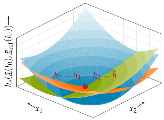
Figure 4. Quality function $h_s\left(\underline{\tilde{x}}\left(t_0\right),{\underline{\tilde{x}}}_{\mathrm{ref}}\left(t_0\right)\right)$ for all $s\in \mathcal{S}=$ {0,1,2} with $t_0>0$.

It can be imagined that the choice of each ${\underline{\underline{M}}}_s\left(t\right)$ is crucial for convergence. For instance, Figure 5 exemplifies an unfavorable and a well-designed parameterization. In both Figure 4 and Figure 5, the color gradient reflects the value of $h_s\left(\underline{\tilde{x}}\left(t_0\right),{\underline{\tilde{x}}}_{\mathrm{ref}}\left(t_0\right)\right)$, with lighter colors representing larger values.

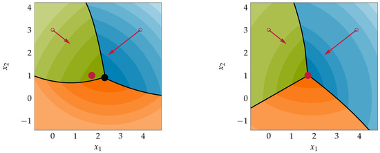
Figure 5. Topview of $h_s\left(\underline{\tilde{x}}\left(t_0\right),{\underline{\tilde{x}}}_{\mathrm{ref}}\left(t_0\right)\right)$ for all $s\in \mathcal{S}=$ {0, 1, 2}, intersection point (black dot) and reference trajectory ${\underline{\tilde{x}}}_{\mathrm{ref}}$ (red dot) with $t_0>0$.

If the switching sequence is created by (10), subsystem 0 or 1 is activated depending on the initial value $\underline{\tilde{x}}\left(0\right)$, marked as circles in Figure 5. As a decrease in $h_s\left(\underline{\tilde{x}}\left(t\right),{\underline{\tilde{x}}}_{\mathrm{ref}}\left(t\right)\right)$ is enforced by (14), when subsystem s is active, the shifted state trajectory $\underline{\tilde{x}}\left(t\right)$ moves in the direction of the arrows until another $h_s\left(\underline{\tilde{x}}\left(t\right),{\underline{\tilde{x}}}_{\mathrm{ref}}\left(t\right)\right)$ exceeds the value of the quality function of the currently active subsystem, marked as black lines in Figure 5. From this point on, the shifted state trajectory $\underline{\tilde{x}}\left(t\right)$ moves along this intersection line in the direction of decreasing $h_s\left(\underline{\tilde{x}}\left(t\right),{\underline{\tilde{x}}}_{\mathrm{ref}}\left(t\right)\right)$, and the system only switches between the subsystems whose quality functions $h_s\left(\underline{\tilde{x}}\left(t\right),{\underline{\tilde{x}}}_{\mathrm{ref}}\left(t\right)\right)$ coincide. The switching behavior along the intersection line is similar to that of a system in sliding mode. Sliding along the intersection line is interrupted only by reaching another intersection line. In Figure 5, this corresponds to the point were all $h_s\left(\underline{\tilde{x}}\left(t\right),{\underline{\tilde{x}}}_{\mathrm{ref}}\left(t\right)\right)$ are equal. At this point, the system switches between all subsystems, and the state trajectory remains in an area around this point. The size of the area represents a design parameter and depends on the maximum allowed switching frequency and the dynamics of the subsystems. In Figure 5a, the unfavorable parameterization of ${\underline{\underline{M}}}_s\left(t\right)$ leads to an intersection point unequal to ${\underline{\tilde{x}}}_{\mathrm{ref}}\left(t\right)$. Only if condition (13) is satisfied, i.e., all matrices ${\underline{\underline{M}}}_s\left(t\right)$ are chosen, such that all $h_s\left(\underline{\tilde{x}}\left(t\right),{\underline{\tilde{x}}}_{\mathrm{ref}}\left(t\right)\right)$ intersect in ${\underline{x}}_{\mathrm{ref}}\left(t\right)$, the convergence to ${\mathcal{R}}_{\delta }^n$ is given; see Figure 5b. The value $\widehat{h}$ of the quality functions at the intersection point is not important for convergence and is related to the choice of each individual ${\underline{\underline{M}}}_s\left(t\right)$. In this publication, it is proposed to define ${\underline{\underline{M}}}_s\left(t\right)$ by

$$\begin{array}{cc}\hfill {\underline{\underline{M}}}_s\left(t\right)& =\frac{\underline{\underline{M}}}{{\left({\underline{\tilde{x}}}_{\mathrm{ref}}\left(t\right)-{\underline{x}}_{\mathrm{eq},s}\right)}^T\underline{\underline{M}}\left({\underline{\tilde{x}}}_{\mathrm{ref}}\left(t\right)-{\underline{x}}_{\mathrm{eq},s}\right)}=\frac{\underline{\underline{M}}}{{\underline{\tilde{x}}}_{\mathrm{ref},s}^T\left(t\right)\underline{\underline{M}}{\underline{\tilde{x}}}_{\mathrm{ref},s}\left(t\right)},\forall s\in \mathcal{S}\hfill \end{array}$$

(16)

with the weighting matrix $\underline{\underline{M}}$ from (5). As ${\underline{\tilde{x}}}_{\mathrm{ref},s}^T\left(t\right)\underline{\underline{M}}{\underline{\tilde{x}}}_{\mathrm{ref},s}\left(t\right)>0,\forall {\underline{\tilde{x}}}_{\mathrm{ref}}\left(t\right)\ne {\underline{x}}_{\mathrm{eq},s},\forall t$ per definition (see (6) and (7)), the time-varying matrices ${\underline{\underline{M}}}_s\left(t\right)$ are positive definite and $h_s\left(\underline{\tilde{x}}\left(t\right),{\underline{\tilde{x}}}_{\mathrm{ref}}\left(t\right)\right)$ fulfills the conditions (11) and (12). With this choice of ${\underline{\underline{M}}}_s\left(t\right)$, the quality functions $h_s\left(\underline{\tilde{x}}\left(t\right),{\underline{\tilde{x}}}_{\mathrm{ref}}\left(t\right)\right)$ become the ratio of the weighted distance between ${\underline{x}}_{\mathrm{eq},s}$ and ${\underline{\tilde{x}}}_{\mathrm{ref}}\left(t\right)$ and $\underline{\tilde{x}}\left(t\right)$, respectively, which are all equal if $\underline{\tilde{x}}\left(t\right)={\underline{\tilde{x}}}_{\mathrm{ref}}\left(t\right)$.

If a switched system with only one subsystem is considered, the condition $h_0\left(\underline{\tilde{x}}\left(t\right),{\underline{\tilde{x}}}_{\mathrm{ref}}\left(t\right)\right)=\widehat{h}$ is given for an infinite number of combinations of ${\underline{\tilde{x}}}_{\mathrm{ref}}\left(t\right)$ and $\underline{\tilde{x}}\left(t\right)$. More precisely, the condition is fulfilled as long as ${\underline{\tilde{x}}}_{\mathrm{ref}}\left(t\right)$ and $\underline{\tilde{x}}\left(t\right)$ are on the same orbit around ${\underline{x}}_{\mathrm{eq},s}$, illustrated as blue curve around ${\underline{x}}_{\mathrm{eq},0}$ in Figure 6 for some $t_0>0$.

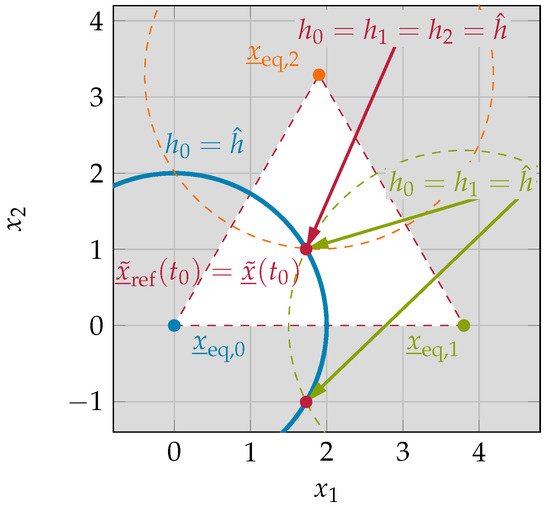
Figure 6. Intersection of $h_s\left(\underline{\tilde{x}}\left(t\right),{\underline{\tilde{x}}}_{\mathrm{ref}}\left(t\right)\right)=\widehat{h}$ for all $s\in \mathcal{S}=$ {0, 1, 2}.

Introducing a second subsystem, the set of solutions reduces to two possible equilibria, specified by the two intersections of the orbits around the two system equilibria ${\underline{x}}_{\mathrm{eq},0}$ and ${\underline{x}}_{\mathrm{eq},1}$, marked as red dots in Figure 6. Finally, again considering the exemplary system with three subsystems shown in Figure 4 or Figure 5b, the quality functions $h_s\left(\underline{\tilde{x}}\left(t\right),{\underline{\tilde{x}}}_{\mathrm{ref}}\left(t\right)\right)$ are all equal to $\widehat{h}$ only at ${\underline{\tilde{x}}}_{\mathrm{ref}}\left(t\right)=\underline{\tilde{x}}\left(t\right)$, i.e., ${\underline{x}}_{\mathrm{ref}}\left(t\right)=\underline{x}\left(t\right)$. Hence, defining the matrices ${\underline{\underline{M}}}_s\left(t\right)$ as suggested in (16), condition (13) is also satisfied for all $s\in \mathcal{S}$.

Taking a closer look at $h_s\left(\underline{\tilde{x}}\left(t\right),{\underline{\tilde{x}}}_{\mathrm{ref}}\left(t\right)\right)$, where all ${\underline{\underline{M}}}_s\left(t\right)$ are specified by (16) and defining

$$\begin{array}{cc}\hfill W_s\left({\underline{\tilde{x}}}_{\mathrm{ref},s}\left(t\right)\right)& ={\underline{\tilde{x}}}_{\mathrm{ref},s}^T\left(t\right)\underline{\underline{M}}{\underline{\tilde{x}}}_{\mathrm{ref},s}\left(t\right),\hfill \end{array}$$

(17)

the quality function becomes

$$\begin{array}{cc}\hfill h_s\left(\underline{\tilde{x}}\left(t\right),{\underline{\tilde{x}}}_{\mathrm{ref}}\left(t\right)\right)& =\frac{V_s({\underline{\tilde{x}}}_{\mathrm{eq},s}\left(t\right))}{W_s\left({\underline{\tilde{x}}}_{\mathrm{ref},s}\left(t\right)\right)}.\hfill \end{array}$$

(18)

Applying the quotient rule, the time derivative of the quality functions follows

$$\begin{array}{cc}\hfill {\dot{h}}_s\left(\underline{\tilde{x}}\left(t\right),{\underline{\tilde{x}}}_{\mathrm{ref}}\left(t\right)\right)& =\frac{{\dot{V}}_s\left({\underline{\tilde{x}}}_{\mathrm{eq},s}\left(t\right)\right)W_s\left({\underline{\tilde{x}}}_{\mathrm{ref},s}\left(t\right)\right)-{\dot{W}}_s\left({\underline{\tilde{x}}}_{\mathrm{ref},s}\left(t\right)\right)V_s\left({\underline{\tilde{x}}}_{\mathrm{eq},s}\left(t\right)\right)}{{\left(W_s\left({\underline{\tilde{x}}}_{\mathrm{ref},s}\left(t\right)\right)\right)}^2}.\hfill \end{array}$$

(19)

Thus, condition (14) is fulfilled as long as the inequality

$$\begin{array}{cc}\hfill \frac{{\dot{W}}_s\left({\underline{\tilde{x}}}_{\mathrm{ref},s}\left(t\right)\right)}{W_s\left({\underline{\tilde{x}}}_{\mathrm{ref},s}\left(t\right)\right)}& >\frac{{\dot{V}}_s\left({\underline{\tilde{x}}}_{\mathrm{eq},s}\left(t\right)\right)}{V_s\left({\underline{\tilde{x}}}_{\mathrm{eq},s}\left(t\right)\right)}\hfill \end{array}$$

(20)

holds. It can be noticed that both quotients in (20) are a measure for the convergence to the subsystem equlibria ${\underline{x}}_{\mathrm{eq},s}$. When $V_s\left({\underline{\tilde{x}}}_{\mathrm{eq},s}\left(t\right)\right)$ is a candidate Lyapunov function and a constant reference point ${\underline{x}}_{\mathrm{ref}}\left(t\right)=\mathrm{const}.$ as well as constant input $\underline{u}\left(t\right)=\mathrm{const}.$ are given, (20) simplifies to the classical Lyapunov stability criterion, where the time derivative of $V_s\left({\underline{\tilde{x}}}_{\mathrm{eq},s}\left(t\right)\right)$ must satisfy ${\dot{V}}_s\left({\underline{\tilde{x}}}_{\mathrm{eq},s}\left(t\right)\right)<0,\forall {\underline{\tilde{x}}}_{\mathrm{eq},s}\left(t\right)$.

2.4. Conditions for Convergence

In summary, the convergence of the state trajectory $x\left(t\right)$ to ${\mathcal{R}}_{\delta }^n$ is given for a switched system in ${\mathbb{R}}^n$, when the following conditions are fulfilled:

C.1

The system consists of subsystems having unique equlibria ${\underline{x}}_{\mathrm{eq},s}$;

C.2

The shifted reference trajectory lies in the subspace ${\mathcal{R}}_{\mathrm{ref}}^n$, i.e., ${\underline{\tilde{x}}}_{\mathrm{ref}}\left(t\right)\in {\mathcal{R}}_{\mathrm{ref}}^n\subset {\mathbb{R}}^n$;

C.3

The switching law $s\left(t\right)$ is given by (10);

C.4

The quality functions $h_s\left(\underline{\tilde{x}}\left(t\right),{\underline{\tilde{x}}}_{\mathrm{ref}}\left(t\right)\right)$ are defined by (18);

C.5

Inequality (20) holds.

3. Converter System Description and Analysis

The further aim of this paper is to describe how the proposed control method can be applied to a practical system. For this purpose, an exemplary power converter system is considered, consisting of a simple two-level VSC with ohmic-inductive filter and an additional sinusoidal voltage source. This system, often found in drive applications or power supply systems [7,13,23], is introduced and transferred to a switched system representation in the following section.

3.1. System Description

3.1.1. Two-Level Voltage Source Converter

Figure 7 shows the circuit diagram of the considered VSC. Assuming ideal switches, the converter output voltage $\underline{u}\left(t\right)={\left[\begin{array}{ccc}{u}_c\left(t\right)& u_b\left(t\right)& u_a\left(t\right)\end{array}\right]}^T$ is given by

$$\begin{array}{cc}\hfill \underline{u}\left(t\right)& =u_{\mathrm{DC}}\left(t\right)·\underline{p}\hfill \end{array}$$

(21)

and the corresponding phase voltage vector ${\underline{u}}_{\mathrm{P}}\left(t\right)={\left[\begin{array}{ccc}{u}_{\mathrm{P},c}\left(t\right)& u_{\mathrm{P},b}\left(t\right)& u_{\mathrm{P},a}\left(t\right)\end{array}\right]}^T$ by

$$\begin{array}{cc}\hfill {\underline{u}}_{\mathrm{P}}\left(t\right)& =\frac{u_{\mathrm{DC}}\left(t\right)}{3}\left[\begin{array}{ccc}2& -1& -1\\ -1& 2& -1\\ -1& -1& 2\end{array}\right]\underline{p}.\hfill \end{array}$$

(22)

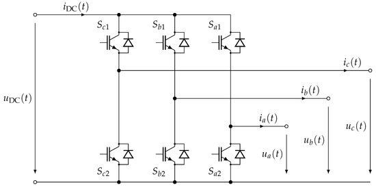
Figure 7. Circuit diagram of a two-level VSC.

Here, the normalized phase potential vector $\underline{p}={\left[\begin{array}{ccc}{p}_c& p_b& p_a\end{array}\right]}^T$, with $p_{c,b,a}\in \left[0,1\right]$, depends on the state of the switches $S_{c1,b1,a1}$ and $S_{c2,b2,a2}$.

Both the voltage space vector $\underline{u}\left(t\right)$ and the corresponding current space vector $\underline{i}\left(t\right)={\left[\begin{array}{ccc}{i}_c\left(t\right)& i_b\left(t\right)& i_a\left(t\right)\end{array}\right]}^T$ can be represented in different coordinate systems, where the most frequently used is the $120{}^{\circ }$ phase coordinate system with the three axes $c,b,a$ and the orthogonal coordinate system with two axes $(\alpha ,\beta )$, which is utilized in this paper. The $\alpha$-axis of this stationary reference system is aligned with the a-phase of the VSC, as shown in the converter hexagon in Figure 8. The converter hexagon is formed by the possible phase potentials $\underline{p}$.

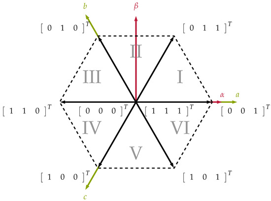
Figure 8. Hexagon of a two-level converter and stationary reference frames.

The unscaled transformation between variables in the $\left(c,b,a\right)$ phase coordinate system, i.e., $x_{c,b,a}\left(t\right)$, and variables in the $(\alpha ,\beta )$ reference frame, i.e., $x_{\alpha ,\beta }\left(t\right)$, is given by [24]

$$\begin{array}{cc}\hfill x_{\alpha }\left(t\right)& =x_a\left(t\right)-\frac{x_b\left(t\right)+x_c\left(t\right)}{2}\hfill \end{array}$$

(23)

$$\begin{array}{cc}\hfill x_{\beta }\left(t\right)& =\frac{\sqrt{3}\left(x_b\left(t\right)-x_c\left(t\right)\right)}{2}.\hfill \end{array}$$

(24)

Considering (21), (23), and (24), the voltage space vector ${\underline{u}}_{\mathrm{P}}\left(t\right)$ in $(\alpha ,\beta )$ reference frame is given by

$$\begin{array}{cc}\hfill u_{\alpha }\left(t\right)& =u_{\mathrm{DC}}\left(t\right)\left(p_a-\frac{p_b+p_c}{2}\right)\hfill \end{array}$$

(25)

$$\begin{array}{cc}\hfill u_{\beta }\left(t\right)& =\frac{\sqrt{3}{u}_{\mathrm{DC}}\left(t\right)\left(p_b-p_c\right)}{2}.\hfill \end{array}$$

(26)

3.1.2. Load Model

The converter load is described by an ohmic-inductive filter and a voltage source. The ohmic-inductive filter part shown in Figure 9 can be used to model the simple output filter plus grid impedance of an electrical power supply system or the stator windings of an electrical machine, where the voltage source corresponds to the grid voltage or the electro magnetic force (EMF), respectively; see, e.g., [7,13,23].

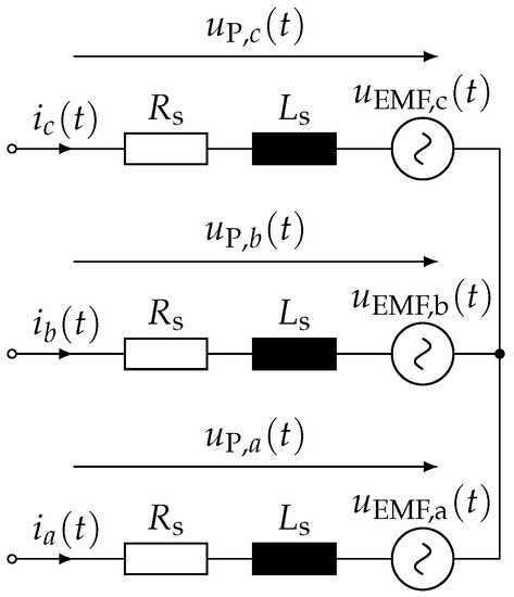
Figure 9. Circuit diagram of the converter load.

In this paper, the load should be given by a symmetrical permanent magnetic synchronous machine (PMSM), which can be modeled by the normalized $(\alpha ,\beta )$ frame voltage equations from [24]

$$\begin{array}{cc}\hfill \frac{d{i}_{\alpha }^{\prime }\left(t\right)}{dt}& =\frac{-1}{T_{\mathrm{s}}}\left(i_{\alpha }^{\prime }\left(t\right)-\frac{u_{\alpha }^{\prime }\left(t\right)}{R^{\prime }}+\frac{u_{\mathrm{EMF},\alpha }}{R^{\prime }}\right)=\frac{-1}{T_{\mathrm{s}}}\left(i_{\alpha }^{\prime }\left(t\right)-\frac{u_{\alpha }^{\prime }\left(t\right)}{R^{\prime }}-c_{\mathrm{EMF}}{\omega }^{\prime }\left(t\right)sin\left(\epsilon \left(t\right)\right)\right)\hfill \end{array}$$

(27)

$$\begin{array}{cc}\hfill \frac{d{i}_{\beta }^{\prime }\left(t\right)}{dt}& =\frac{-1}{T_{\mathrm{s}}}\left(i_{\beta }^{\prime }\left(t\right)-\frac{u_{\beta }^{\prime }\left(t\right)}{R^{\prime }}+\frac{u_{\mathrm{EMF},\beta }}{R^{\prime }}\right)=\frac{-1}{T_{\mathrm{s}}}\left(i_{\beta }^{\prime }\left(t\right)-\frac{u_{\beta }^{\prime }\left(t\right)}{R^{\prime }}+c_{\mathrm{EMF}}{\omega }^{\prime }\left(t\right)cos\left(\epsilon \left(t\right)\right)\right)\hfill \end{array}$$

(28)

using the normalized values

$$\begin{array}{ccccccccccc}\hfill u^{\prime }& =& \frac{u}{u_{\mathrm{nom}}}\hfill & ,& \hfill i^{\prime }& =& \frac{i}{i_{\mathrm{nom}}}\hfill & ,& \hfill {\omega }^{\prime }& =& \frac{\omega }{{\omega }_{\mathrm{nom}}}\hfill \\ \hfill R^{\prime }& =& \frac{R_{\mathrm{s}}·i_{\mathrm{nom}}}{u_{\mathrm{nom}}}\hfill & ,& \hfill L^{\prime }& =& \frac{L_{\mathrm{s}}·i_{\mathrm{nom}}}{u_{\mathrm{nom}}}\hfill & ,& \hfill T_{\mathrm{s}}& =& \frac{L^{\prime }}{R^{\prime }}\hfill \end{array}$$

(29)

where $u_{\mathrm{nom}}$ is the machine’s nominal voltage, $i_{\mathrm{nom}}$ is the machine’s nominal current, and $c_{\mathrm{EMF}}$ defines the EMF constant

$$\begin{array}{cc}\hfill c_{\mathrm{EMF}}& =\frac{z_p{\mathsf{\Phi }}_F{\omega }_{\mathrm{nom}}}{L^{\prime }{u}_{\mathrm{nom}}}{T}_{\mathrm{s}}.\hfill \end{array}$$

(30)

Here, $R_{\mathrm{s}}$ and $L_{\mathrm{s}}$ are the resistance and inductance of a stator winding, respectively, ${\omega }_{\mathrm{nom}}$ specifies the machine’s nominal angular frequency, ${\mathsf{\Phi }}_F$ is the permanent magnetic excitation, and $z_p$ is the number of pole pairs. The EMF constant $c_{\mathrm{EMF}}$ in combination with normalized angular frequency ${\omega }^{\prime }\left(t\right)$, i.e., the last term in (27) and (28), respectively, defines the normalized current caused by the EMF. The electrical angle, and thus, the position of the rotor, are represented by $\epsilon \left(t\right)$, specified by

$$\begin{array}{cc}\hfill \frac{d{\omega }^{\prime }\left(t\right)}{dt}& =\frac{2{\mathsf{\Phi }}_F{z}_p{i}_{\mathrm{nom}}}{3\mathsf{\Theta }{\omega }_{\mathrm{nom}}}\left(cos\left(\epsilon \left(t\right)\right)i_{\beta }^{\prime }\left(t\right)-sin\left(\epsilon \left(t\right)\right)i_{\alpha }^{\prime }\left(t\right)\right)-\frac{m_{\mathrm{L}}\left(t\right)}{\mathsf{\Theta }{\omega }_{\mathrm{nom}}}\hfill \end{array}$$

(31)

$$\begin{array}{cc}\hfill \frac{d\epsilon \left(t\right)}{dt}& =z_p{\omega }_{\mathrm{nom}}{\omega }^{\prime }\left(t\right),\hfill \end{array}$$

(32)

where $m_{\mathrm{L}}\left(t\right)$ and $\mathsf{\Theta }$ are the load torque and rotor inertia, respectively. Since the dynamics of the mechanical machine part are slow compared with the dynamics of the electrical part, the EMF is usually considered to be a slowly varying but independent disturbance in the current control loop; see, e.g., [4]. Moreover, (31) and (32) are not considered in the following. In this paper, the load and the VSC are analyzed as one system. By combining (25), (26), (27), and (28), the interconnected system can be described by

$$\begin{array}{cc}\hfill \frac{d{i}_{\alpha }^{\prime }\left(t\right)}{dt}& =\frac{-1}{T_{\mathrm{s}}}\left(i_{\alpha }^{\prime }\left(t\right)-\frac{p_a-\frac{p_b+p_c}{2}}{R^{\prime }}{u}_{\mathrm{DC}}^{\prime }\left(t\right)-c_{\mathrm{EMF}}{\omega }^{\prime }\left(t\right)sin\left(\epsilon \left(t\right)\right)\right)\hfill \end{array}$$

(33)

$$\begin{array}{cc}\hfill \frac{d{i}_{\beta }^{\prime }\left(t\right)}{dt}& =\frac{-1}{T_{\mathrm{s}}}\left(i_{\beta }^{\prime }\left(t\right)-\frac{\sqrt{3}\left(p_b-p_c\right)}{2R^{\prime }}{u}_{\mathrm{DC}}^{\prime }\left(t\right)+c_{\mathrm{EMF}}{\omega }^{\prime }\left(t\right)cos\left(\epsilon \left(t\right)\right)\right).\hfill \end{array}$$

(34)

All parameters mentioned above, as well as the DC link voltage $u_{\mathrm{DC}}^{\prime }$, are assumed to be constant in the following.

3.2. Switched System Representation

3.2.1. State Space Model

Observing (33) and (34), it becomes clear that the dynamics of the system depend on the vector $\underline{p}$, and thus, on the switching state of the inverter. Due to the control of the switches by a PWM, the system exhibits both switching behavior and continuous dynamics. To cope with this intrinsic switching behavior of the phase potentials, the system in (33) and (34) is described as a switched system with subsystems of the form in (2) with the state space vector

$$\begin{array}{cc}\hfill \underline{x}\left(t\right)& =\left[\begin{array}{c}{i}_{\alpha }^{\prime }\left(t\right)\\ i_{\beta }^{\prime }\left(t\right)\end{array}\right].\hfill \end{array}$$

(35)

Consequently, the system matrix $\underline{\underline{A}}$ is given by

$$\begin{array}{cc}\hfill \underline{\underline{A}}& =\left[\begin{array}{cc}-\frac{1}{T_{\mathrm{s}}}& 0\\ 0& -\frac{1}{T_{\mathrm{s}}}\end{array}\right],\hfill \end{array}$$

(36)

the subsystem equilibria ${\underline{x}}_{\mathrm{eq},s}$ by

$$\begin{array}{cc}\hfill {\underline{x}}_{\mathrm{eq},s}& =\frac{u_{\mathrm{DC}}^{\prime }}{R^{\prime }}\left[\begin{array}{c}{p}_a-\frac{p_b+p_c}{2}\\ \frac{\sqrt{3}\left(p_b-p_c\right)}{2}\end{array}\right],\hfill \end{array}$$

(37)

and, with $\underline{\underline{B}}=\underline{\underline{A}}$, the input $\underline{u}\left(t\right)$ is equal to the normalized current caused by the EMF. In case of a normal operation, where it can be assumed that the angular frequency ${\omega }^{\prime }$ is constant, it follows

$$\begin{array}{cc}\hfill \underline{u}\left(t\right)& ={\underline{i}}_{\mathrm{EMF}}^{\prime }\left(t\right)=c_{\mathrm{EMF}}{\omega }^{\prime }\left[\begin{array}{c}-sin(z_p{\omega }^{\prime }{\omega }_{\mathrm{nom}}t+{\epsilon }_0)\\ cos(z_p{\omega }^{\prime }{\omega }_{\mathrm{nom}}t+{\epsilon }_0)\end{array}\right],\hfill \end{array}$$

(38)

where it is assumed that the angular frequency ${\omega }^{\prime }$ is constant.

Within this system representation, each possible vector $\underline{p}$ defines one subsystem. The assignment of a given vector $\underline{p}$ to the respective subsystem is given by

$$\begin{array}{cc}\hfill s& =4·p_c+2·p_b+1·p_a.\hfill \end{array}$$

(39)

Due to the structure of the VSC, the vectors $\underline{p}={\left[\begin{array}{ccc}0& 0& 0\end{array}\right]}^T$ and $\underline{p}={\left[\begin{array}{ccc}1& 1& 1\end{array}\right]}^T$ imply the same voltage to the load. Under the condition that each subsystem has a unique equilibrium, both vectors are treated as subsystem 0, i.e., $s\in \mathcal{S}=\left\{0,1,\cdots ,6\right\}$.

3.2.2. Shifted State Trajectory

According to the definitions above and the state transformations of (3) and (6), it follows

$$\begin{array}{cc}\hfill {\underline{\tilde{x}}}_{\mathrm{eq},s}\left(t\right)& =\underline{x}\left(t\right)+{\underline{i}}_{\mathrm{EMF}}^{\prime }\left(t\right)-{\underline{x}}_{\mathrm{eq},s}\hfill \\ \hfill & = \left[\begin{array}{c}{i}_{\alpha }^{\prime }\left(t\right)\\ i_{\beta }^{\prime }\left(t\right)\end{array}\right] + c_{\mathrm{EMF}}{\omega }^{\prime }\left[\begin{array}{c}-sin(z_p{\omega }^{\prime }{\omega }_{\mathrm{nom}}t+{\epsilon }_0)\\ cos(z_p{\omega }^{\prime }{\omega }_{\mathrm{nom}}t+{\epsilon }_0)\end{array}\right]-\frac{u_{\mathrm{DC}}^{\prime }}{R^{\prime }}\left[\begin{array}{c}{p}_a-\frac{p_b+p_c}{2}\\ \frac{\sqrt{3}\left(p_b-p_c\right)}{2}\end{array}\right].\hfill \end{array}$$

(40)

Furthermore, its time derivative is given by

$$\begin{array}{cc}\hfill {\dot{\underline{\tilde{x}}}}_{\mathrm{eq},s}\left(t\right)& =\dot{\underline{x}}\left(t\right)+{\dot{{\underline{i}}^{\prime }}}_{\mathrm{EMF}}\left(t\right)-{\dot{\underline{x}}}_{\mathrm{eq},s}\hfill \\ \hfill & =\underline{\underline{A}}{\underline{\tilde{x}}}_{\mathrm{eq},s}\left(t\right)+{\underline{\underline{A}}}_{\mathrm{EMF}}{\underline{i}}_{\mathrm{EMF}}^{\prime }\left(t\right)-\underline{0},\hfill \end{array}$$

(41)

where ${\underline{\underline{A}}}_{\mathrm{EMF}}$ is given by

$$\begin{array}{cc}\hfill {\underline{\underline{A}}}_{\mathrm{EMF}}& =\left[\begin{array}{cc}0& -z_p{\omega }^{\prime }{\omega }_{\mathrm{nom}}\\ z_p{\omega }^{\prime }{\omega }_{\mathrm{nom}}& 0\end{array}\right].\hfill \end{array}$$

(42)

Since a quadratic function of the form given by (9) is assigned to each subsystem for all $s\in \mathcal{S}$,

$$\begin{array}{cc}\hfill {\dot{V}}_s\left({\underline{\tilde{x}}}_{\mathrm{eq},s}\left(t\right)\right)& ={\underline{\tilde{x}}}_{\mathrm{eq},s}^T\left(t\right)\underline{\underline{M}}{\dot{\underline{\tilde{x}}}}_{\mathrm{eq},s}\left(t\right)+{\dot{\underline{\tilde{x}}}}_{\mathrm{eq},s}^T\left(t\right)\underline{\underline{M}}{\underline{\tilde{x}}}_{\mathrm{eq},s}\left(t\right)\hfill \end{array}$$

(43)

applies. Including (36), (41), and (42) and introducing $\underline{\underline{M}}$ as a diagonal matrix, it follows

$$\begin{array}{cc}\hfill {\dot{V}}_s\left({\underline{\tilde{x}}}_{\mathrm{eq},s}\left(t\right)\right)& ={\underline{\tilde{x}}}_{\mathrm{eq},s}^T\left(t\right)\left(\underline{\underline{M}}\underline{\underline{A}}+{\underline{\underline{A}}}^T\underline{\underline{M}}\right){\underline{\tilde{x}}}_{\mathrm{eq},s}\left(t\right)\hfill \\ & \phantom{=}+{\underline{\tilde{x}}}_{\mathrm{eq},s}^T\left(t\right)\underline{\underline{M}}{\underline{\underline{A}}}_{\mathrm{EMF}}{\underline{i}}_{\mathrm{EMF}}^{\prime }\left(t\right)+{\underline{i}}_{\mathrm{EMF}}^T\left(t\right){\underline{\underline{A}}}_{\mathrm{EMF}}^T\underline{\underline{M}}{\underline{\tilde{x}}}_{\mathrm{eq},s}\left(t\right)\hfill \end{array}$$

(44)

$$=-\frac{2}{T_{\mathrm{s}}}{\underline{\tilde{x}}}_{\mathrm{eq},s}^T\left(t\right)\underline{\underline{M}}{\underline{\tilde{x}}}_{\mathrm{eq},s}\left(t\right)+2{\underline{\tilde{x}}}_{\mathrm{eq},s}^T\left(t\right)\underline{\underline{M}}{\underline{\underline{A}}}_{\mathrm{EMF}}{\underline{i}}_{\mathrm{EMF}}^{\prime }\left(t\right).$$

(45)

3.2.3. Reference Trajectory

As a circle around the origin in the $(\alpha ,\beta )$-plane is a common reference trajectory of the system under consideration, ${\underline{x}}_{\mathrm{ref}}\left(t\right)$ can usually be defined by

$$\begin{array}{cc}\hfill {\underline{x}}_{\mathrm{ref}}\left(t\right)& ={\widehat{x}}_{\mathrm{ref}}\left[\begin{array}{c}-sin\left(z_p{\omega }_{\mathrm{ref}}^{\prime }{\omega }_{\mathrm{nom}}t+{\epsilon }_{\mathrm{ref},0}\right)\\ cos\left(z_p{\omega }_{\mathrm{ref}}^{\prime }{\omega }_{\mathrm{nom}}t+{\epsilon }_{\mathrm{ref},0}\right)\end{array}\right],\hfill \end{array}$$

(46)

and thus, the shifted reference trajectory ${\underline{\tilde{x}}}_{\mathrm{ref}}\left(t\right)$ becomes

$$\begin{array}{cc}{\underline{\tilde{x}}}_{\mathrm{ref}}\left(t\right)\hfill & ={\underline{x}}_{\mathrm{ref}}\left(t\right)+{\underline{i}}_{\mathrm{EMF}}^{\prime }\left(t\right).\hfill \end{array}$$

(47)

By choosing this reference trajectory, its derivative is given by

$$\begin{array}{cc}\hfill {\dot{\underline{\tilde{x}}}}_{\mathrm{ref}}\left(t\right)& =\left[\begin{array}{cc}0& -z_p{\omega }_{\mathrm{ref}}^{\prime }{\omega }_{\mathrm{nom}}\\ z_p{\omega }_{\mathrm{ref}}^{\prime }{\omega }_{\mathrm{nom}}& 0\end{array}\right]{\underline{x}}_{\mathrm{ref}}\left(t\right)+\left[\begin{array}{cc}0& -z_p{\omega }^{\prime }{\omega }_{\mathrm{nom}}\\ z_p{\omega }^{\prime }{\omega }_{\mathrm{nom}}& 0\end{array}\right]{\underline{i}}_{\mathrm{EMF}}^{\prime }\left(t\right)\hfill \\ \hfill & ={\underline{\underline{A}}}_{\mathrm{ref}}{\underline{x}}_{\mathrm{ref}}\left(t\right)+{\underline{\underline{A}}}_{\mathrm{EMF}}{\underline{i}}_{\mathrm{EMF}}^{\prime }\left(t\right).\hfill \end{array}$$

(48)

Furthermore, the energy function of the reference trajectory $W_s\left({\underline{\tilde{x}}}_{\mathrm{ref},s}\left(t\right)\right)$ is given by (17). With (7) and (48), its time derivative ${\dot{W}}_s\left({\underline{\tilde{x}}}_{\mathrm{ref},s}\left(t\right)\right)$ is defined by

$$\begin{array}{cc}\hfill {\dot{W}}_s\left({\underline{\tilde{x}}}_{\mathrm{ref},s}\left(t\right)\right)& ={\underline{\tilde{x}}}_{\mathrm{ref},s}^T\left(t\right)\underline{\underline{M}}{\dot{\underline{\tilde{x}}}}_{\mathrm{ref},s}\left(t\right)+{\dot{\underline{\tilde{x}}}}_{\mathrm{ref},s}^T\left(t\right)\underline{\underline{M}}{\underline{\tilde{x}}}_{\mathrm{ref},s}\left(t\right)\hfill \\ \hfill & ={\underline{\tilde{x}}}_{\mathrm{ref},s}^T\left(t\right)\underline{\underline{M}}\left({\dot{\underline{\tilde{x}}}}_{\mathrm{ref}}\left(t\right)-\underline{0}\right)+{\left({\dot{\underline{\tilde{x}}}}_{\mathrm{ref}}\left(t\right)-\underline{0}\right)}^T\underline{\underline{M}}{\underline{\tilde{x}}}_{\mathrm{ref},s}\left(t\right)\hfill \\ \hfill & ={\underline{\tilde{x}}}_{\mathrm{ref},s}^T\left(t\right)\underline{\underline{M}}\left({\underline{\underline{A}}}_{\mathrm{ref}}{\underline{x}}_{\mathrm{ref}}\left(t\right)+{\underline{\underline{A}}}_{\mathrm{EMF}}{\underline{i}}_{\mathrm{EMF}}^{\prime }\left(t\right)\right)\hfill \\ \hfill & \phantom{=}+{\left({\underline{\underline{A}}}_{\mathrm{ref}}{\underline{x}}_{\mathrm{ref}}\left(t\right)+{\underline{\underline{A}}}_{\mathrm{EMF}}{\underline{i}}_{\mathrm{EMF}}^{\prime }\left(t\right)\right)}^T\underline{\underline{M}}{\underline{\tilde{x}}}_{\mathrm{ref},s}\left(t\right).\hfill \end{array}$$

(49)

Choosing $\underline{\underline{M}}$ as diagonal matrix, it follows

$$\begin{array}{cc}\hfill {\dot{W}}_s\left({\underline{\tilde{x}}}_{\mathrm{ref},s}\left(t\right)\right)& =2{\underline{\tilde{x}}}_{\mathrm{ref},s}^T\left(t\right)\underline{\underline{M}}\left({\underline{\underline{A}}}_{\mathrm{ref}}{\underline{x}}_{\mathrm{ref}}\left(t\right)+{\underline{\underline{A}}}_{\mathrm{EMF}}{\underline{i}}_{\mathrm{EMF}}^{\prime }\left(t\right)\right).\hfill \end{array}$$

(50)

3.3. Analysis of Convergence Conditions

In the following section, the conditions C.1 to C.5 given in Section 2 are checked for the given system.

3.3.1. System Preconditions

Due to the switched system representation described above, C.1 is given. Furthermore, the subspace ${\mathcal{R}}_{\mathrm{ref}}^2$ spanned by the ${\underline{x}}_{\mathrm{eq},s}$ is a hexagon in the $(\alpha ,\beta )$-plane with an edge length of $\frac{u_{\mathrm{DC}}^{\prime }}{R^{\prime }}$; see Figure 10.

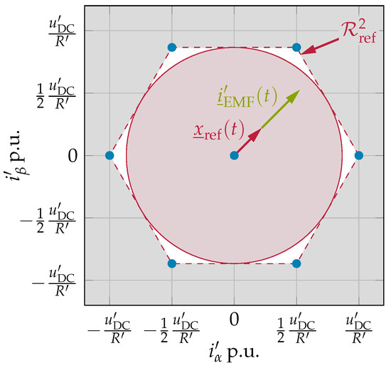
Figure 10. Location of ${\underline{x}}_{\mathrm{eq},s}\forall s\in \mathcal{S}$ with ${\underline{i}}_{\mathrm{EMF}}^{\prime }\left(t\right)$ in the $(\alpha ,\beta )$-plane, corresponding ${\mathcal{R}}_{\mathrm{ref}}^2$ and one possible ${\underline{x}}_{\mathrm{ref}}\left(t\right)$.

In the following, the shifted reference trajectory ${\underline{\tilde{x}}}_{\mathrm{ref}}\left(t\right)$ is bounded by

$$\begin{array}{cc}\hfill \left|\left|{\underline{\tilde{x}}}_{\mathrm{ref}}\left(t\right)\right|\right|& \le {\widehat{x}}_{\mathrm{ref}}+c_{\mathrm{EMF}}{\omega }^{\prime }\le \frac{\sqrt{3}}{2}\frac{u_{\mathrm{DC}}^{\prime }}{R^{\prime }}\hfill \end{array}$$

(51)

on the red circle shown in Figure 10. This boundary ensures that ${\underline{\tilde{x}}}_{\mathrm{ref}}\left(t\right)\in {\mathcal{R}}_{\mathrm{ref}}^2$ is given at any time. Thus, C.2 is satisfied.

Furthermore, C.3 is given by applying the switching law (10) to the system under consideration and with $h_s\left(\underline{\tilde{x}}\left(t\right),{\underline{\tilde{x}}}_{\mathrm{ref}}\left(t\right)\right)$ defined by (19) for all $s\in \mathcal{S}$, C.4 is also fulfilled.

3.3.2. Derivation of the Quality Function

Finally, it is necessary to check whether (20) is given, to ensure that C.5 is also true.

Substituting (9), (17), (45), and (50) in (20) yields

$$\begin{array}{cc}\hfill \frac{{\dot{W}}_s\left({\underline{\tilde{x}}}_{\mathrm{ref},s}\left(t\right)\right)}{W_s\left({\underline{\tilde{x}}}_{\mathrm{ref},s}\left(t\right)\right)}& >\frac{{\dot{V}}_s\left({\underline{\tilde{x}}}_{\mathrm{eq},s}\left(t\right)\right)}{V_s\left({\underline{\tilde{x}}}_{\mathrm{eq},s}\left(t\right)\right)}\hfill \\ \hfill \frac{2{\underline{\tilde{x}}}_{\mathrm{ref},s}^T\left(t\right)\underline{\underline{M}}\left({\underline{\underline{A}}}_{\mathrm{ref}}{\underline{x}}_{\mathrm{ref}}\left(t\right)+{\underline{\underline{A}}}_{\mathrm{EMF}}{\underline{i}}_{\mathrm{EMF}}^{\prime }\left(t\right)\right)}{{\underline{\tilde{x}}}_{\mathrm{ref},s}^T\left(t\right)\underline{\underline{M}}{\underline{\tilde{x}}}_{\mathrm{ref},s}\left(t\right)}& >\frac{-\frac{2}{T_{\mathrm{s}}}{\underline{\tilde{x}}}_{\mathrm{eq},s}^T\left(t\right)\underline{\underline{M}}{\underline{\tilde{x}}}_{\mathrm{eq},s}\left(t\right)+2{\underline{\tilde{x}}}_{\mathrm{eq},s}^T\left(t\right)\underline{\underline{M}}{\underline{\underline{A}}}_{\mathrm{EMF}}{\underline{i}}_{\mathrm{EMF}}^{\prime }\left(t\right)}{{\underline{\tilde{x}}}_{\mathrm{eq},s}^T\left(t\right)\underline{\underline{M}}{\underline{\tilde{x}}}_{\mathrm{eq},s}\left(t\right)}.\hfill \end{array}$$

(52)

An analytical solution of (52) that is valid in the entire state space is possible under certain conditions, but it is very complex and usually not necessary. Especially when, as in the present system, the state trajectory is limited by physical constraints and superimposed control circuits to a small region of the total state space. Therefore, it is not pursued further here and (52) is selectively verified for the relevant cases.

If ${\underline{i}}_{\mathrm{EMF}}^{\prime }\left(t\right)$ and ${\underline{x}}_{\mathrm{ref}}\left(t\right)$ are given by (38) and (46), respectively, where

$$\begin{array}{cc}\hfill {\omega }_{\mathrm{ref}}^{\prime }& ={\omega }^{\prime }\hfill \end{array}$$

(53)

$$\begin{array}{cc}\hfill {\epsilon }_{\mathrm{ref},0}& ={\epsilon }_0\hfill \end{array}$$

(54)

$$\begin{array}{cc}\hfill \left|\left|\underline{x}\left(t\right)\right|\right|& <<\frac{u_{\mathrm{DC}}^{\prime }}{R^{\prime }},\hfill \end{array}$$

(55)

with (53), (54), (55) and the definitions of ${\underline{\underline{A}}}_{\mathrm{ref}}$, the convergence condition in (52) simplifies to

$$\begin{array}{cc}\hfill \frac{2{\underline{\tilde{x}}}_{\mathrm{ref},s}^T\left(t\right)\underline{\underline{M}}\left({\underline{\underline{A}}}_{\mathrm{ref}}{\underline{x}}_{\mathrm{ref}}\left(t\right)+{\underline{\underline{A}}}_{\mathrm{EMF}}{\underline{i}}_{\mathrm{EMF}}^{\prime }\left(t\right)\right)}{{\underline{\tilde{x}}}_{\mathrm{ref},s}^T\left(t\right)\underline{\underline{M}}{\underline{\tilde{x}}}_{\mathrm{ref},s}\left(t\right)}& >\frac{-\frac{2}{T_{\mathrm{s}}}{\underline{\tilde{x}}}_{\mathrm{eq},s}^T\left(t\right)\underline{\underline{M}}{\underline{\tilde{x}}}_{\mathrm{eq},s}\left(t\right)+2{\underline{\tilde{x}}}_{\mathrm{eq},s}^T\left(t\right)\underline{\underline{M}}{\underline{\underline{A}}}_{\mathrm{EMF}}{\underline{i}}_{\mathrm{EMF}}^{\prime }\left(t\right)}{{\underline{\tilde{x}}}_{\mathrm{eq},s}^T\left(t\right)\underline{\underline{M}}{\underline{\tilde{x}}}_{\mathrm{eq},s}\left(t\right)}\hfill \\ \hfill \frac{2\left(\frac{{\widehat{x}}_{\mathrm{ref}}}{c_{\mathrm{EMF}}{\omega }^{\prime }}+1\right){\underline{\tilde{x}}}_{\mathrm{ref},s}^T\left(t\right)\underline{\underline{M}}{\underline{\underline{A}}}_{\mathrm{EMF}}{\underline{i}}_{\mathrm{EMF}}^{\prime }\left(t\right)}{{\underline{\tilde{x}}}_{\mathrm{ref},s}^T\left(t\right)\underline{\underline{M}}{\underline{\tilde{x}}}_{\mathrm{ref},s}\left(t\right)}& >\frac{-\frac{2}{T_{\mathrm{s}}}{\underline{\tilde{x}}}_{\mathrm{eq},s}^T\left(t\right)\underline{\underline{M}}{\underline{\tilde{x}}}_{\mathrm{eq},s}\left(t\right)+2{\underline{\tilde{x}}}_{\mathrm{eq},s}^T\left(t\right)\underline{\underline{M}}{\underline{\underline{A}}}_{\mathrm{EMF}}{\underline{i}}_{\mathrm{EMF}}^{\prime }\left(t\right)}{{\underline{\tilde{x}}}_{\mathrm{eq},s}^T\left(t\right)\underline{\underline{M}}{\underline{\tilde{x}}}_{\mathrm{eq},s}\left(t\right)}\hfill \\ \hfill 2\left(\frac{{\widehat{x}}_{\mathrm{ref}}}{c_{\mathrm{EMF}}{\omega }^{\prime }}+1\right)\frac{{\underline{\tilde{x}}}_{\mathrm{ref},s}^T\left(t\right)\underline{\underline{M}}{\underline{\underline{A}}}_{\mathrm{EMF}}{\underline{i}}_{\mathrm{EMF}}^{\prime }\left(t\right)}{{\underline{\tilde{x}}}_{\mathrm{ref},s}^T\left(t\right)\underline{\underline{M}}{\underline{\tilde{x}}}_{\mathrm{ref},s}\left(t\right)}& >-\frac{2}{T_{\mathrm{s}}}+2\frac{{\underline{\tilde{x}}}_{\mathrm{eq},s}^T\left(t\right)\underline{\underline{M}}{\underline{\underline{A}}}_{\mathrm{EMF}}{\underline{i}}_{\mathrm{EMF}}^{\prime }\left(t\right)}{{\underline{\tilde{x}}}_{\mathrm{eq},s}^T\left(t\right)\underline{\underline{M}}{\underline{\tilde{x}}}_{\mathrm{eq},s}\left(t\right)}.\hfill \end{array}$$

(56)

Choosing $\underline{\underline{M}}=\underline{\underline{I}}$, to weight all state variables equally, and inserting ${\underline{\underline{A}}}_{\mathrm{EMF}}$ and ${\underline{i}}_{\mathrm{EMF}}^{\prime }\left(t\right)$, after some transformations, it follows

$$\begin{array}{c}\hfill \frac{\left(\frac{{\widehat{x}}_{\mathrm{ref}}}{{\omega }^{\prime }{c}_{\mathrm{EMF}}}+1\right)\frac{u_{\mathrm{DC}}^{\prime }}{R^{\prime }}{\omega }^{{\prime }^2}{z}_p{\omega }_{\mathrm{nom}}{c}_{\mathrm{EMF}}\left(p_{\alpha }cos\left(\epsilon \left(t\right)\right)+p_{\beta }sin\left(\epsilon \left(t\right)\right)\right)}{{\left|\left|{\underline{\tilde{x}}}_{\mathrm{ref},s}\left(t\right)\right|\right|}^2}\\ \hfill >\\ \hfill -\frac{1}{T_{\mathrm{s}}}+\frac{\frac{u_{\mathrm{DC}}^{\prime }}{R^{\prime }}{\omega }^{{\prime }^2}{z}_p{\omega }_{\mathrm{nom}}{c}_{\mathrm{EMF}}}{{\left|\left|{\underline{\tilde{x}}}_{\mathrm{eq},s}\left(t\right)\right|\right|}^2}\left(p_{\alpha }cos\left(\epsilon \left(t\right)\right)+p_{\beta }sin\left(\epsilon \left(t\right)\right)\right)\end{array}$$

(57)

with $p_{\alpha }$ from (A1) and $p_{\beta }$ from (A2). By inserting $p_{\alpha }$ and $p_{\beta }$ from Table A1 for $s=0$, (57) simplifies to

$$\begin{array}{cc}\hfill 0& >-\frac{1}{T_{\mathrm{s}}}\hfill \end{array}$$

(58)

for subsystem 0. As $T_{\mathrm{s}}>0$, (58) holds independently of system parameters and reference trajectory. For all other subsystems, i.e., $s\in \mathcal{S}\backslash 0$, (57) can be simplified to

$$\begin{array}{cc}\hfill \frac{{\left({\widehat{x}}_{\mathrm{ref}}+{\omega }^{\prime }{c}_{\mathrm{EMF}}-\frac{u_{\mathrm{DC}}^{\prime }}{R^{\prime }}\right)}^2}{\left|{\omega }^{\prime }\right|\left|{\widehat{x}}_{\mathrm{ref}}\right|}& >\frac{T_{\mathrm{s}}{u}_{\mathrm{DC}}^{\prime }{z}_p{\omega }_{\mathrm{nom}}}{R^{\prime }}\hfill \end{array}$$

(59)

using the transformations shown in Appendix A. The condition in (59) is valid for all $s\in \mathcal{S}\backslash 0$. Subsystem 0 still has no constraints; consequently, (59) is the only constraint among the possible reference trajectories.

In summary, C.5 is true for all reference trajectories ${\underline{x}}_{\mathrm{ref}}\left(t\right)$ according to (47) with parameters ${\omega }^{\prime }$, ${\omega }_{\mathrm{ref}}^{\prime }$, ${\epsilon }_0$, ${\epsilon }_{\mathrm{ref},0}$, and ${\widehat{x}}_{\mathrm{ref}}$ satisfying (53), (54), (55), and (59).

4. Simulative Verification

In order to verify the proposed control method, the converter system from Section 3 is simulated in MATLAB/Simulink^®. The linear system in (33) and (34) is transformed into the $\left(c,b,a\right)$ phase coordinate system and implemented. A time variant reference trajectory ${\underline{x}}_{\mathrm{ref}}\left(t\right)$, as defined in (47), is transferred to the presented hysteresis current control. This set-up is simulated with the aim to assess the current ripple and the switching frequency behavior. Since the maximum switching frequency in the practical application is limited by the semiconductors of the inverter, it is utilized as design criterion. The simulation set-up is implemented with the simulation parameters listed in Table 1.

Table 1. Simulation parameter.

Parameter	Value
MATLAB® version	9.3
Simulink® version	9.0
solver type	variable step
solver name	ode23s

4.1. Simulation Set Up

Figure 11 shows the simulation block diagram implemented with the values from Table 2.

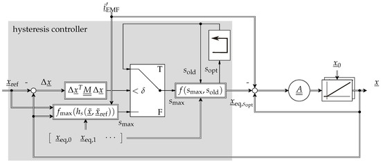
Figure 11. Implemented simulation set-up.

Table 2. System constants and exemplary normalized values for simulative verification.

System Constant	Symbol	Value	Unit
normalized DC Link voltage	$u_{\mathrm{DC}}^{\prime }$	$2.273$	−
number of pole pair	$z_p$	2	−
nominal speed	${\omega }_{\mathrm{nom}}$	$3.142\times {10}^2$	$\frac{1}{s}$
flux leakage	${\mathsf{\Phi }}_F$	$0.587$	$Vs$
normalized stator resistance	$R^{\prime }$	$0.334\times {10}^{-2}$	−
normalized stator inductance	$L^{\prime }$	$9.155\times {10}^{-5}$	s
normalized stator time constant	$T_{\mathrm{s}}$	$2.744\times {10}^{-2}$	s
EMF constant	$c_{\mathrm{EMF}}$	$2.957\times {10}^2$	−

The utilized switching law $f_{\max }\left(h_s\left(\underline{\tilde{x}},{\underline{\tilde{x}}}_{\mathrm{ref}}\right)\right)$ is defined by

$$\begin{array}{cc}\hfill f_{\max }\left(h_s\left(\underline{\tilde{x}},{\underline{\tilde{x}}}_{\mathrm{ref}}\right)\right)& =\left\{\begin{array}{cc}arg\left(\underset{s\in \mathcal{S}}{max}\left(h_s\left(\underline{\tilde{x}}\left(t\right),{\underline{\tilde{x}}}_{\mathrm{ref}}\left(t\right)\right)\right)\right),& \forall t>t_{\delta ,1}\\ arg\left({maxhyst}_{s\in \mathcal{S}}\left(h_s\left(\underline{\tilde{x}}\left(t\right),{\underline{\tilde{x}}}_{\mathrm{ref}}\left(t\right)\right)\right)\right),& \forall t\le t_{\delta ,1}\end{array}\right.\hfill \end{array}$$

(60)

where $t_{\delta ,1}$ denotes the first time $\underline{x}\left(t\right)$ moves into ${\mathcal{R}}_{\delta }^2$. The function $maxhyst\left(·\right)$ represents a $max\left(·\right)$-function extended by a hysteresis with the hysteresis threshold ${\delta }_{\mathrm{hyst}}$. Thus, a change of the output only takes place when the previous maximum value is exceeded by ${\delta }_{\mathrm{hyst}}$. This prevents high frequency switching along the intersection lines. Both hysteresis thresholds where heuristically set such that the switching frequency $f_{\mathrm{SW},c,b,a}$ of the phases are in the common frequency range of a VSC from $40$ Hz to $40$ kHz [6]. Furthermore, the function $f\left(s_{\max },s_{\mathrm{old}}\right)$ with two outputs $s_{\mathrm{opt}}$ and ${\underline{x}}_{\mathrm{eq},s_{\mathrm{opt}}}$ is utilized to distinguish between the two vectors $\underline{p}={\left[\begin{array}{ccc}0& 0& 0\end{array}\right]}^T$ and $\underline{p}={\left[\begin{array}{ccc}1& 1& 1\end{array}\right]}^T$ and generate the corresponding subsystem equilibrium ${\underline{x}}_{\mathrm{eq},s_{\mathrm{opt}}}$. Depending on the previous subsystem $s_{\mathrm{old}}$, $s_{\mathrm{opt}}$ is defined by

$$\begin{array}{cc}\hfill s_{\mathrm{opt}}& =\left\{\begin{array}{cc}{s}_{\max },& \forall s_{\max }\ne 0\\ 0,& \forall s_{\max }=0 \wedge \left(s_{\mathrm{old}}=0\vee s_{\mathrm{old}}=1\vee s_{\mathrm{old}}=2\vee s_{\mathrm{old}}=4\right)\\ 7,& \forall s_{\max }=0 \wedge \left(s_{\mathrm{old}}=3\vee s_{\mathrm{old}}=5\vee s_{\mathrm{old}}=6\vee s_{\mathrm{old}}=7\right)\end{array}\right..\hfill \end{array}$$

(61)

The subsystem equilibrium ${\underline{x}}_{\mathrm{eq},s_{\mathrm{opt}}}$ is given by (37), where $\underline{p}$ and $s_{\mathrm{opt}}$ fulfill (39).

In a first simulation, the transient behavior of the presented approach is demonstrated. For this purpose, the reference trajectory is defined by

$$\begin{array}{cc}\hfill {\underline{x}}_{\mathrm{ref}}\left(t\right)& =1.5·\left[\begin{array}{c}-sin\left(z_p{\omega }_{\mathrm{nom}}t\right)\\ cos\left(z_p{\omega }_{\mathrm{nom}}t\right)\end{array}\right],\hfill \end{array}$$

(62)

and the initial value by

$$\begin{array}{cc}\hfill {\underline{x}}_0& =\left[\begin{array}{c}0\\ 0\end{array}\right].\hfill \end{array}$$

(63)

Additional simulations are performed with the reference trajectory ${\underline{x}}_{\mathrm{ref}}\left(t\right)$ defined in (47), initial values specified by

$$\begin{array}{cccc}\hfill {\underline{x}}_0& ={\widehat{x}}_{\mathrm{ini}}{\left[\begin{array}{cc}-sin\left(\frac{\pi }{6}k\right)& cos\left(\frac{\pi }{6}k\right)\end{array}\right]}^T\hfill & \hfill & \forall k=0,1,\dots ,11\hfill \end{array}$$

(64)

and the constants listed in Table 3.

Table 3. Parameters for the reference trajectory, initial values, and hysteresis control.

Constant	Symbol	Value	Unit
normalized reference speed	${\omega }_{\mathrm{ref}}^{\prime }$	1	−
normalized actual speed	${\omega }^{\prime }$	1	−
normalized reference amplitude	${\widehat{x}}_{\mathrm{ref}}$	$1.5$	−
initial reference angle	${\epsilon }_{\mathrm{ref},0}$	0	$\mathrm{rad}$
normalized initial amplitude	${\widehat{x}}_{\mathrm{ini}}$	$2.5$	−
hysteresis threshold of ${\mathcal{R}}_{\delta }^2$	$\delta$	$3.24\times {10}^{-2}$	−
hysteresis threshold of $maxhyst\left(·\right)$	${\delta }_{\mathrm{hyst}}$	$0.10\times {10}^{-2}$	−

According to Section 3.3.2, the convergence is given if and only if (53), (54), (55), and (59) hold with the values from Table 3. Inserting the corresponding values in (59) leads to

$$\begin{array}{cc}\hfill \frac{{\left({\widehat{x}}_{\mathrm{ref}}+{\omega }^{\prime }{c}_{\mathrm{EMF}}-\frac{u_{\mathrm{DC}}^{\prime }}{R^{\prime }}\right)}^2}{\left|{\omega }^{\prime }\right|\left|{\widehat{x}}_{\mathrm{ref}}\right|}& >\frac{T_{\mathrm{s}}{u}_{\mathrm{DC}}^{\prime }{z}_p{\omega }_{\mathrm{nom}}}{R^{\prime }}\hfill \\ \hfill \frac{{\left(1.5+\left(2.957-\frac{2.273}{0.334}\right)·{10}^2\right)}^2}{1.5}& >\frac{3.142·2·2.744·2.273}{0.334}·{10}^2\hfill \\ \hfill 9.797·{10}^4& >1.173·{10}^4.\hfill \end{array}$$

(65)

Thus, the convergence to ${\mathcal{R}}_{\delta }^2$ is theoretically given.

4.2. Simulation Results

4.2.1. Trajectory Convergence

The results of the first simulation shown in Figure 12 indicate a fast transient response of the state trajectory $\underline{x}\left(t\right)$ to the reference trajectory ${\underline{x}}_{\mathrm{ref}}\left(t\right)$. Due to the selected initial value ${\underline{x}}_0$, the state trajectory $\underline{x}\left(t\right)$ moves along the $\beta$-axis in the direction of the reference trajectory ${\underline{x}}_{\mathrm{ref}}\left(t\right)$ and reaches the target environment ${\mathcal{R}}_{\delta }^2$ after a few switching events; see Figure 12a. From Figure 12b, it can be seen that the entire transient process is completed after $0.15 \mathrm{m}\mathrm{s}$.

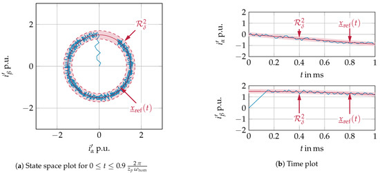
Figure 12. State trajectory $\underline{x}\left(t\right)$ for reference trajectory ${\underline{x}}_{\mathrm{ref}}\left(t\right)$ by (62) and initial value ${\underline{x}}_0$ by (63).

The results of the other simulations are shown in Figure 13. In Figure 13a, the state trajectories for all initial values are given in the state space. In addition, Figure 13b shows the trajectories of the state variables $i_{\alpha }^{\prime }$ and $i_{\beta }^{\prime }$ over time t with one representative initial value $\left(k=11\right)$.

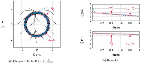
Figure 13. State trajectories $x\left(t\right)$ for different initial values ${\underline{x}}_0$ and same reference trajectory ${\underline{x}}_{\mathrm{ref}}\left(t\right)$.

As can be verified, the hysteresis current controller is able to guarantee the convergence of the state trajectories $\underline{x}\left(t\right)$ into ${\mathcal{R}}_{\delta }^2$ regardless of the initial values ${\underline{x}}_0$; see Figure 13a. In addition, the fast transient response typical for the hysteresis processes is shown. The state trajectory enters ${\mathcal{R}}_{\delta }^2$ at $t_{\delta ,1}=0.05 \mathrm{m}\mathrm{s}$; see Figure 13b.

4.2.2. Current Ripple

For the evaluation of the current ripple, the current in the $\left(c,b,a\right)$ phase coordinate system is examined. Figure 14 shows both the deviation of the phase current from the respective reference frame $\mathsf{\Delta }{i}_{c,b,a}^{\prime }$ and the corresponding spectrum.

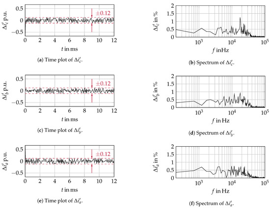
Figure 14. Time plot and spectra of phase current ripple.

It can be seen from Figure 14a,c,e that the ripples of the phase currents are at no time greater than 12% of the nominal current. In addition, Figure 14b,d,f shows a broad spectrum with values smaller than the 2% nominal current. The total harmonic distortion (THD) of the currents, defined by

$$\begin{array}{cc}\hfill {\mathrm{THD}}_I& =\sqrt{{\left(\frac{I}{I_1}\right)}^2-1}\hfill \end{array}$$

(66)

according to [25], is used as a quality criterion. Here, I denotes the sum of root mean square values (RMS) of the current harmonics and $I_1$ the RMS of its fundamental component, considering harmonic components up to the 50th order [26]. The values listed in Table 4 are below the limit of 5% nominal current required in [26] for all phases.

Table 4. Phase current THD for all phases.

System Constant	Symbol	Value			Unit
phase number		c	b	a	−
current THD	${\mathrm{THD}}_{I,c,b,a}$	$3.201$	$3.123$	$3.119$

4.3. Switching Behavior

For the practical application of the hysteresis controller, the maximum switching frequency is an important parameter, since it is limited by the semiconductors used in the converter. Here, not the frequency of switching between the subsystems but the switching frequency of the individual phases of the converter is critical. Since this is equivalent to a change of the potential of the corresponding element of the vector $\underline{p}$, the instantaneous switching frequency $f_{\mathrm{SW},c,b,a}$ of the phases is determined by a period measurement between two positive edges of $p_{c,b,a}$. As with all hysteresis-based methods, the switching frequency is not constant. The switching frequency behavior can be characterized by the maximum ${\widehat{f}}_{\mathrm{SW},c,b,a}$, average ${\overline{f}}_{\mathrm{SW},c,b,a}$, and minimum switching frequency ${\check{f}}_{\mathrm{SW},c,b,a}$; see Table 5.

Table 5. Switching frequency values for all phases.

System Constant	Symbol	Value			Unit
phase number		c	b	a	−
maximum switching frequency	${\widehat{f}}_{\mathrm{SW},c,b,a}$	$38.760$	$32.787$	$32.787$	$\mathrm{kHz}$
average switching frequency	${\overline{f}}_{\mathrm{SW},c,b,a}$	$18.662$	$16.432$	$18.117$	$\mathrm{kHz}$
minimum switching frequency	${\check{f}}_{\mathrm{SW},c,b,a}$	$1.810$	$1.861$	$2.013$	$\mathrm{kHz}$

On the one hand, it can be seen that the required frequency band is maintained on all three phases. On the other hand, the different values on the individual phases indicate different loads on the corresponding semiconductors.

Since these values only represent the switching frequency behavior to a limited extent, the time curves of the instantaneous switching frequencies $f_{\mathrm{SW},c,b,a}$ are shown in Figure 15.

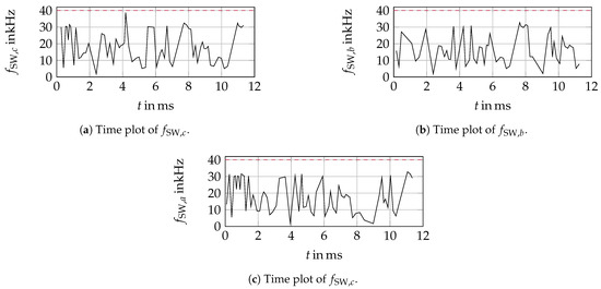
Figure 15. Switching frequency $f_{\mathrm{SW},c,b,a}$ of positive potential on each phase.

The curves show a similar behavior on all three phases, which are also shifted by $120{}^{\circ }$ to each other due to the $120{}^{\circ }$ phase shift between the currents.

5. Discussion

In this paper, a novel hysteresis-based current control approach was presented. The basis of the developed control approach is the theory of switching systems, in particular, the system class of switching systems with multiple equilibria. The special feature of this system class is that each stable subsystem converges to its own equilibrium when it is active. This property allows the state trajectory $\underline{x}\left(t\right)$ to converge to a reference trajectory ${\underline{x}}_{\mathrm{ref}}\left(t\right)$ by an appropriate switching between these subsystems. In the first part of this paper, it was shown that the presented approach minimizes the quality functions $h_s\left(\underline{\tilde{x}}\left(t\right),{\underline{\tilde{x}}}_{\mathrm{ref}}\left(t\right)\right)$ for all $s\in \mathcal{S}$ by applying the switching law (10). Furthermore, it was shown that reaching the minimum $\widehat{h}$ is equivalent to the convergence of the state trajectory $\underline{x}\left(t\right)$ to the reference trajectory ${\underline{x}}_{\mathrm{ref}}\left(t\right)$. To prevent high-frequency switching at the reference trajectory, an environment ${\mathcal{R}}_{\delta }^n$ around ${\underline{x}}_{\mathrm{ref}}\left(t\right)$ was introduced where no switching occurs. To illustrate the applicability of the presented approach to a practical system, an example application consisting of a voltage source converter plus load was introduced in the second part of the paper. After adapting the system to the above-mentioned system class, the applicability of the presented approach was shown by verifying the conditions established in Section 2.2. In the simulations subsequently shown, the control approach was extended by the additional hysteresis threshold ${\delta }_{\mathrm{hyst}}$. This is necessary to prevent the high-frequency switching along the intersection curves of two subsystems discussed in Section 2.2. However, the simulations shown confirm that the sliding mode, and thus, the use of the second hysteresis, occur only for a very short period. Thus, the state trajectory is within the target environment ${\mathcal{R}}_{\delta }^2$ after a very short time. Consequently, the switching behavior of the control approach is largely determined by the introduced hysteresis width $\delta$. The presented approach also shows a reasonable current ripple and current oscillation range while maintaining a low average switching frequency compared with other well-known control strategies.

However, a reduction of the hysteresis width, and thus, the current oscillation range are not possible due to the large oscillation range of the switching frequencies, which limits the applicability of the new controller. The variable switching frequency is a challenge for EMI investigations. On the one hand, the switching energy is distributed over a broad spectrum so that peaks do not occur at individual frequencies. On the other hand, an exact switching frequency prediction is necessary to exclude the fact that the expected switching frequencies do not scatter into blocked frequency ranges. A meaningful EMI analysis can therefore only be performed after developing an algorithm to observe or to predict the switching frequency during runtime. As with all hysteresis-based methods, a fast sampling rate of the ADCs and an equally fast clock rate of the controller are necessary to precisely maintain the hysteresis limits in practical implementations. Especially, the need to calculate all quality functions in each sampling step increases the computational power requirements of the approach. By using an FPGA with a sufficient number of mutlipliers, this computation can be paralleled, thus reducing the cycle time of the algorithm. The maximal search can then be performed by simple logical operations.

References

- Kim, H.G.; Sul, S.K.; Park, M.H. Optimal Efficiency Drive of a Current Source Inverter Fed Induction Motor by Flux Control. IEEE Trans. Ind. Appl. 1984, IA-20, 1453–1459. [Google Scholar] [CrossRef]
- Mademlis, C.; Kioskeridis, I.; Margaris, N. Optimal Efficiency Control Strategy for Interior Permanent-Magnet Synchronous Motor Drives. IEEE Trans. Energy Convers. 2004, 19, 715–723. [Google Scholar] [CrossRef]
- Ta, C.M.; Hori, Y. Convergence improvement of efficiency-optimization control of induction motor drives. IEEE Trans. Ind. Appl. 2001, 37, 1746–1753. [Google Scholar] [CrossRef]
- Hans, F.; Schumacher, W.; Chou, S.F.; Wang, X. Design of Multifrequency Proportional-Resonant Current Controllers for Voltage-Source Converters. IEEE Trans. Power Electron. 2020. [Google Scholar] [CrossRef]
- Suul, J.A.; Ljokelsoy, K.; Midtsund, T.; Undeland, T. Synchronous Reference Frame Hysteresis Current Control for Grid Converter Applications. IEEE Trans. Ind. Appl. 2011, 47, 2183–2194. [Google Scholar] [CrossRef]
- Homann, M. Hochdynamische Strom- und Spannungsregelung von Permanenterregten Synchronmaschinen auf Basis vonDelta-Sigma Bitströmen. Ph.D. Thesis, TU Braunschweig, Braunschweig, Germany, 2016. [Google Scholar]
- Thielmann, M.; Klein, A.; Homann, M.; Schumacher, W. Analysis of instantaneous switching frequency of a hysteresis based PWM for control of power electronics. In PCIM Europe 2017; International Exhibition and Conference for Power Electronics, Intelligent Motion, Renewable Energy and Energy Management; VDE VERLAG GMBH: Berlin, Germany, 2017; pp. 390–397. [Google Scholar]
- Mohseni, M.; Islam, S.M. A New Vector-Based Hysteresis Current Control Scheme for Three-Phase PWM Voltage-Source Inverters. IEEE Trans. Power Electron. 2010, 25, 2299–2309. [Google Scholar] [CrossRef]
- Ho, C.M.; Cheung, V.; Chung, H.H. Constant-Frequency Hysteresis Current Control of Grid-Connected VSI Without Bandwidth Control. IEEE Trans. Power Electron. 2009, 24, 2484–2495. [Google Scholar] [CrossRef]
- Klarmann, K.; Thielmann, M.; Schumacher, W. Comparison of Hysteresis Based PWM Schemes ΔΣ-PWM and Direct Torque Control. Appl. Sci. 2021, 11, 2293. [Google Scholar] [CrossRef]
- Hans, F.; Oeltze, M.; Schumacher, W. A Modified ZOH Model for Representing the Small-Signal PWM Behavior in Digital DC-AC Converter Systems. In Proceedings of the IECON 2019-45th Annual Conference of the IEEE Industrial Electronics Society, Lisbon, Portugal, 14–17 October 2019; Volume 1, pp. 1514–1520. [Google Scholar]
- Holmes, D.G. Pulse Width Modulation for Power Converters: Principles and Practice by D. Grahame Homes and Thomas A. Lipo; IEEE Series on Power Engineering; Wiley/Blackwell: Hoboken, NJ, USA, 2003. [Google Scholar]
- Hans, F. Input Admittance Modeling and Passivity-Based Stabilization of Digitally Current-Controlled Grid-Connected Converters. Ph.D. Thesis, Technische Universität Braunschweig, Braunschweig, Germany, 25 June 2021. [Google Scholar]
- Liberzon, D. Switching in Systems and Control; Systems & Control, Birkhäuser: Boston, MA, USA, 2003. [Google Scholar]
- Daafouz, J.; Riedinger, P.; Iung, C. Stability analysis and control synthesis for switched systems: A switched Lyapunov function approach. IEEE Trans. Autom. Control 2002, 47, 1883–1887. [Google Scholar] [CrossRef]
- Lin, H.; Antsaklis, P.J. Stability and Stabilizability of Switched Linear Systems: A Survey of Recent Results. IEEE Trans. Autom. Control 2009, 54, 308–322. [Google Scholar] [CrossRef]
- Yang, G.; Liberzon, D. Input-to-state stability for switched systems with unstable subsystems: A hybrid Lyapunov construction. In Proceedings of the 2014 IEEE 53rd Annual Conference on Decision and Control (CDC), Los Angeles, CA, USA, 15–17 December 2014; pp. 6240–6245. [Google Scholar] [CrossRef]
- Veer, S.; Poulakakis, I. Switched Systems With Multiple Equilibria Under Disturbances: Boundedness and Practical Stability. IEEE Trans. Autom. Control 2020, 65, 2371–2386. [Google Scholar] [CrossRef]
- Mastellone, S.; Stipanovic, D.M.; Spong, M.W. Stability and convergence for systems with switching equilibria. In Proceedings of the 2007 46th IEEE Conference on Decision and Control, New Orleans, LA, USA, 12–14 December 2007; pp. 4013–4020. [Google Scholar] [CrossRef]
- Yuan, S.; Lv, M.; Baldi, S.; Zhang, L. Lyapunov-equation-based stability analysis for switched linear systems and its application to switched adaptive control. IEEE Trans. Autom. Control. 2020. [Google Scholar] [CrossRef]
- Sun, J.; Chen, J. A survey on Lyapunov-based methods for stability of linear time-delay systems. Front. Comput. Sci. 2017, 11, 555–567. [Google Scholar] [CrossRef]
- Cao, Y.; Xu, Y.; Li, Y.; Yu, J.; Yu, J. A Lyapunov Stability Theory-Based Control Strategy for Three-Level Shunt Active Power Filter. Energies 2017, 10, 112. [Google Scholar] [CrossRef] [Green Version]
- Brüske, S. Bauleistungsvergleich und Neutralpunkt-Balancierung für 3-Level-Wechselrichtertopologien für den Einsatz in Elektrofahrzeugen. Ph.D. Thesis, Christian-Albrechts-Universität zu Kiel, Kiel, Germany, 15 September 2016. [Google Scholar]
- Leonhard, W. Control of Electrical Drives, 3rd ed.; Power Systems; Springer: Berlin, Germany, 2001. [Google Scholar]
- IEEE Standard Definitions for the Measurement of Electric Power Quantities Under Sinusoidal, Nonsinusoidal, Balanced, or Unbalanced Conditions. Revis. IEEE Std. 2010, 1459–2000. [CrossRef] [Green Version]
- IEEE Recommended Practice and Requirements for Harmonic Control in Electric Power Systems; University of Campania “Luigi Vanvitelli”: Caserta, Italy, 2014. [CrossRef]
Publisher’s Note: MDPI stays neutral with regard to jurisdictional claims in published maps and institutional affiliations. |
© 2021 by the authors. Licensee MDPI, Basel, Switzerland. This article is an open access article distributed under the terms and conditions of the Creative Commons Attribution (CC BY) license (https://creativecommons.org/licenses/by/4.0/).