EAR-Net: Efficient Atrous Residual Network for Semantic Segmentation of Street Scenes Based on Deep Learning

Abstract

Segmentation of street scenes is a key technology in the field of autonomous vehicles. However, conventional segmentation methods achieve low accuracy because of the complexity of street landscapes. Therefore, we propose an efficient atrous residual network (EAR-Net) to improve accuracy while maintaining computation costs. First, we performed feature extraction and restoration, utilizing depthwise separable convolution (DSConv) and interpolation. Compared with conventional methods, DSConv and interpolation significantly reduce computation costs while minimizing performance degradation. Second, we utilized residual learning and atrous spatial pyramid pooling (ASPP) to achieve high accuracy. Residual learning increases the ability to extract context information by preventing the problem of feature and gradient losses. In addition, ASPP extracts additional context information while maintaining the resolution of the feature map. Finally, to alleviate the class imbalance between the image background and objects and to improve learning efficiency, we utilized focal loss. We evaluated EAR-Net on the Cityscapes dataset, which is commonly used for street scene segmentation studies. Experimental results showed that the EAR-Net had better segmentation results and similar computation costs as the conventional methods. We also conducted an ablation study to analyze the contributions of the ASPP and DSConv in the EAR-Net.

1. Introduction

Nowadays, segmentation and object detection are primarily used in such fields as machine vision, remote sensing images, and medical image analysis, and play an important role in many applications [1,2,3]. The segmentation of street scenes is a key technology in the field of autonomous vehicles, especially in advanced driver assistance systems [4]. There are various types of segmentation, such as semantic segmentation and instance segmentation [5]. In this study, we focus on semantic segmentation, which is a technique for classifying categories of objects and pixels constituting the objects in an image. However, semantic segmentation does not distinguish objects of the same category from each other, and a technique to further classify them is called panoptic segmentation [6].

The complex landscape, different textures, and ambient light in the images pose a challenge to these segmentation techniques. Since the introduction of deep learning algorithms, semantic segmentation has developed rapidly [7]. Deep learning-based semantic segmentation methods using convolutional neural networks (CNNs) have been extensively studied. Representative methods include fully convolutional networks (FCNs) [8], U-Net [9,10,11,12], and DeepLab [13,14,15,16]; these are designed with an encoder–decoder [17,18] structure. The encoder extracts features from the input image and compresses them to generate context information, and the decoder expands the feature map, including context information, and outputs a segmentation map. The context information is essential for classifying object categories, and the segmentation map indicates the category to which each pixel in the image corresponds.

FCN was first proposed as a deep learning-based semantic segmentation method and presented a strategy for using a network for classification in segmentation. However, in FCN, the outline or detailed information is lost in the process of generating the segmentation map; thus, the objects in the image are inaccurately divided. Therefore, various methods, such as U-Net, SegNet, and DeepLab, were proposed to solve this problem. The U-Net is a concatenation operation [19], which minimizes information loss by utilizing the intermediate feature information of the encoder in the decoder. As a result, segmentation accuracy is improved, compared to the FCN. However, U-Net has a problem in that object segmentation is incorrect or fails due to a lack of context information extracted from the encoder. This problem hinders the recognition of the position and motion of the objects in the application field of autonomous vehicles and increases the error of the position and size of lesions when applied to medical image analysis. To improve the segmentation accuracy, four versions (V1, V2, V3, V3+) of DeepLab were developed, and DeepLab continues to be studied: DeepLabv1 proposed an atrous convolution that can increase the kernel size while maintaining the computation costs and applied it to a CNN; DeepLabv2 proposed atrous spatial pyramid pooling (ASPP) to utilize multi-scale features by applying atrous convolution; DeepLabv3 improved the segmentation accuracy by analyzing and improving the previously proposed methods; and DeepLabv3+ improved the decoder and used a modified Xception [20] network as its backbone network.

However, the above methods focus on accuracy and are difficult to use in mobile or embedded devices because of their high computation costs. To solve this problem, ENet [21], ICNet [22], and others are used to minimize the computation costs. In the ENet, a tiny encoder–decoder was designed to achieve very small computation costs. However, as there is a trade-off between accuracy and computation costs, the accuracy was significantly reduced. The accuracy reduction due to the trade-off was minimized in the ICNet by using a multi-scale input strategy and cascaded network. A method proposed by Han et al. [4] achieved a good balance between accuracy and computational complexity by proposing an attention mechanism and class-aware edge information utilization.

In this study, we propose an efficient atrous residual network (EAR-Net) to improve the segmentation accuracy while maintaining the computation costs of previous studies [8,9,22,23]. Our model consists of three modules (residual learning, lightweight ASPP and decoder). First, we achieved high accuracy by utilizing residual learning that enhances the context information extraction ability. The implementation of residual learning is ResNet [24], and we prevented feature map resolution reduction by removing a pooling layer from a stem block pre-processing the input image of the ResNet. This method improves the accuracy with a simple operation, and maintains the residual learning structure, allowing reuse of pre-trained weights on ImageNet. In addition, there is an advantage that this method can be simply applied to other segmentation models. Second, we utilized lightweight ASPP to minimize computation costs. The conventional ASPP greatly contributes to the improvement of segmentation accuracy, but has a disadvantage in that the computation costs are large. Therefore, we minimized the computation costs by replacing traditional convolution with depthwise separable convolution (DSConv) [25] in ASPP. ASPP using DSConv has the advantage that there is almost no decrease in accuracy, which is a trade-off for reducing the computation costs. Third, we proposed a new decoder combining DSConv and interpolation to minimize the computation costs. The decoder performs feature restoration to generate a segmentation map, and a good balance between accuracy and computation costs is important. DSConv and interpolation significantly reduce computation costs while minimizing performance degradation. The decoder consists of three decoding blocks, and aims to further improve accuracy by gradually performing feature map expansion and restoration. Finally, we adopted focal loss [26] to alleviate the class imbalance between the background and the objects. The focal loss increased learning efficiency. The experimental results showed high accuracy with computation costs similar to those in the conventional segmentation methods. In an ablation study, we analyzed the contributions of the ASPP and DSConv in the EAR-Net. The main contributions of this paper are as follows.

• We propose an encoder, utilizing residual learning with improved stem block. This method improves accuracy with a simple operation, can reuse pre-trained weights, and is applicable to other segmentation models;
• We propose a lightweight ASPP utilizing DSConv to minimize the computation costs without degrading accuracy;
• We propose a new efficient decoder combining DSConv and interpolation to achieve a good balance between accuracy and computation costs.

2. Related Work

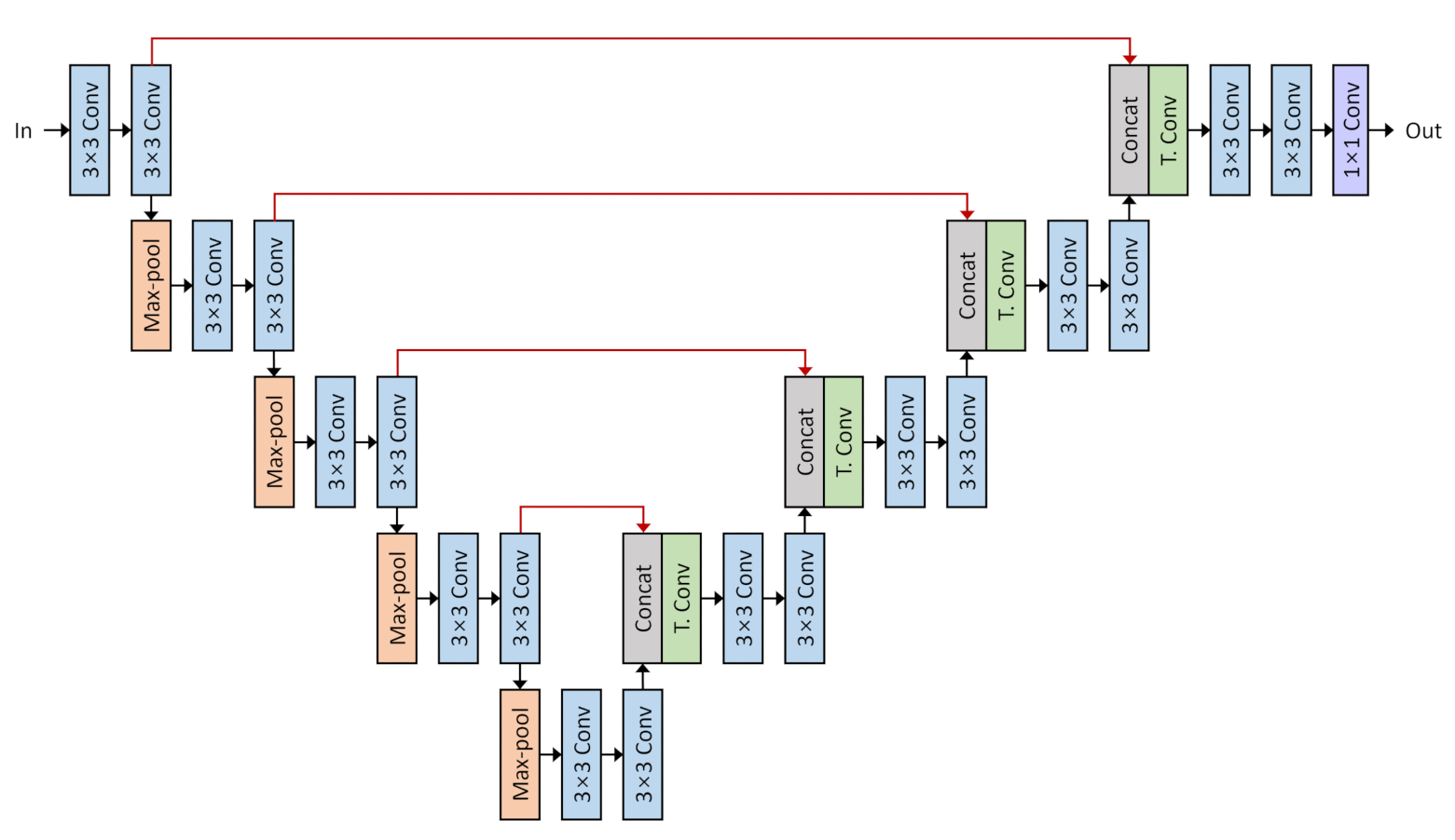
2.1. U-Net

U-Net is a U-shaped network designed for segmentation, which has an encoder–decoder structure. To solve the problem of the FCN, U-Net utilizes the feature information of each step with the concatenation operation and refines the feature information with the subsequent convolution operation. Figure 1 shows the structure of a U-Net. In Figure 1, the left part is the encoder, and the right part is the decoder. The encoder consists of two convolutions and one pooling for each step, and the decoder consists of one transposed convolution and two convolutions. In the concatenation operation, the feature map of each step is connected with the feature map of the corresponding step in the decoder that has undergone transposed convolution to form one feature map. U-Net has significantly fewer convolutions compared to other networks (e.g., ResNet [24] and Xception); there are only 10 convolutions in the encoder, 2 for each step. This causes segmentation inaccuracy because the encoder’s ability to extract context information is low.

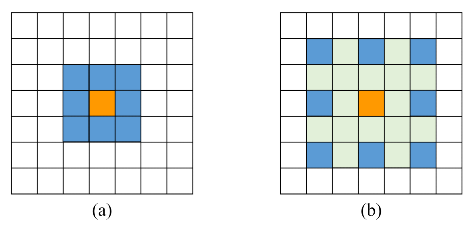
2.2. Atrous Convolution

Atrous convolution is a method to expand the receptive field and was proposed in the DeepLab [14]. The receptive field is an area that a convolution kernel can process in a single operation. When the receptive field is expanded, the area processed by the kernel, that is, the field-of-view, is expanded, which is advantageous for extracting context information. However, for this, the kernel size must be expanded, so the number of parameters and the amount of computation increase. Therefore, atrous convolution, which can expand the receptive field while maintaining the number of parameters and the amount of computation, was studied. Atrous convolution can effectively have a wide receptive field by treating the space between the kernel that is extended (e.g., the light green area in Figure 2b), according to the rate being 0. Figure 2 shows a diagram of atrous convolution. In Figure 2b, only blue and orange pixels are used for the actual convolution operation, and the remaining pixels are treated as 0. Therefore, the computation costs are equal to Figure 2a, but the receptive field is expanded to 5 × 5. Equation (1) represents atrous convolution. In Equation (1), $x,y,w,i,r$ are the input, output, kernel, kernel position, and rate, respectively.

$$y\left[i\right]=\sum _{k}x[i+r·k]w\left[k\right]$$

(1)

2.3. Depthwise Separable Convolution

Depthwise separable convolution (DSConv) is an operation that significantly reduces the computation costs and parameters while minimizing performance degradation, compared to traditional convolution. This computation was adopted in many recent deep learning models and contributes to the intelligence of mobile devices [23,27,28,29]. In traditional convolution, the kernel handles the channel and spatial dimensions simultaneously. However, the DSConv processes the two dimensions separately, and multiple kernels share the parameters required for spatial dimension processing. The DSConv consists of depthwise and pointwise convolution. Depthwise convolution processes spatial dimensions by performing convolution for each channel independently. In contrast, the pointwise convolution processes the channel dimension by combining the outputs of the depthwise convolution into a 1 × 1 kernel. Figure 3 shows a diagram of DSConv.

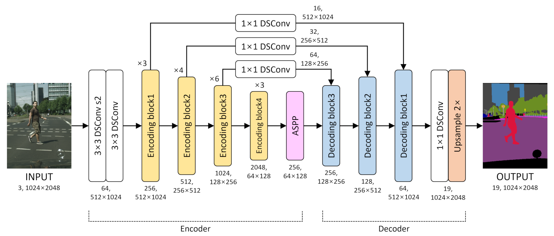
3. Proposed Method

The EAR-Net is composed of an encoder to extract context information and a decoder to generate a precise segmentation map. Figure 4 shows the structure of the EAR-Net.

The encoder consists of 16 encoding blocks with residual learning and 1 ASPP, and the decoder consists of 3 decoding blocks with 1 concatenation operation and 2 consecutive convolutions. The resolution of the feature map output from the decoder is $\frac{1}{2}$ smaller than that of an input image. Moreover, the number of channels in the corresponding feature map exceeds the number of categories in the dataset. Therefore, after matching the number of channels in the feature map using a 1 × 1 convolution, the final segmentation map was generated by upsampling twice. The details of each layer in EAR-Net are introduced in Section 3.1, Section 3.2 and Section 3.3.

3.1. Encoder for Extracting Features

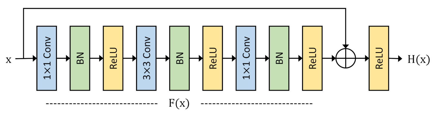
3.1.1. Residual Learning

As shown in Figure 4, the EAR-Net is an encoder–decoder structure. The EAR-Net adopts ResNet with residual learning applied from the encoder to the backbone network. Residual learning prevents the feature loss that occurs during feature extraction and compression of continuous convolutions. Further, it prevents the vanishing gradient problem, which tends to occur as the network becomes deeper. There are several types of ResNets, such as ResNet-18, ResNet-50, and ResNet-101. In ResNet-n, n is the number of layers in the network, and as n increases, the computation cost increases and the performance improves. In this study, we adopted ResNet-50, considering the trade-off between the segmentation performance and speed.

In Figure 4, the backbone network was divided into four blocks (encoding block1, encoding block2, encoding block3, and encoding block4), according to the resolution of the feature map. The blocks have $\frac{1}{2},\frac{1}{4},\frac{1}{8},\frac{1}{16}$ resolution of the input image, respectively. The structure of each encoding block is the same, and Equation (2) and Figure 5 show the encoding block.

$$H\left(x\right)=F\left(x\right)+x$$

(2)

A typical CNN proceeds with stem blocks before proceeding with encoding blocks. A stem block reduces the resolution of the input image and extracts features, such as contours, to reduce the amount of computation of the subsequent convolution. A conventional ResNet reduces the resolution of the feature map to $\frac{1}{4}$ by performing a 7 × 7 traditional convolution with stride 2 and max-pooling. In addition, several semantic segmentation methods perform this down-sampling process while using the ResNet as a backbone. However, this process causes loss of the spatial information included in the feature map. Therefore, the EAR-Net reduces the resolution of the feature map by half by removing max-pooling. Moreover, a 7 × 7 traditional convolution requires much computation due to the large kernel. Therefore, the proposed method replaces the 7 × 7 traditional convolution with two 3 × 3 traditional convolutions. Unless noted otherwise, batch normalization and rectified linear unit (ReLU) layers are included after the convolution layer.

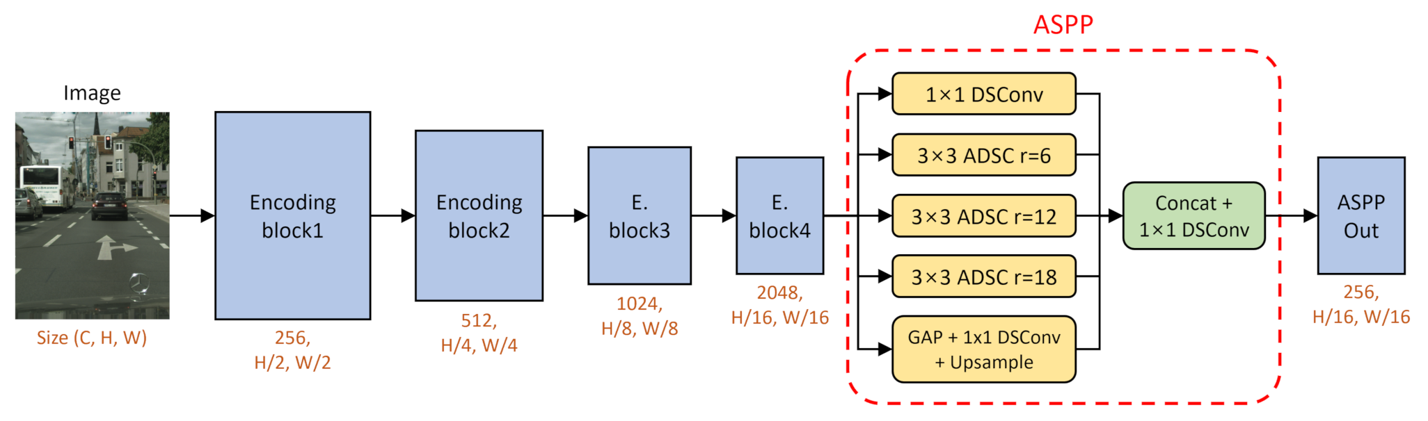
3.1.2. Atrous Spatial Pyramid Pooling

A general CNN reduces the spatial resolution of the feature map by using max-pooling or stride in the continuous convolution process to extend the receptive field and reduce the computation costs. However, this process causes loss of spatial information in the deep layer, thereby reducing the accuracy in pixel unit prediction (e.g., semantic segmentation). Therefore, the EAR-Net utilizes ASPP at the end of the encoder to extend the receptive field without reducing the resolution of the feature map. The ASPP was first presented in DeepLab, and it used several atrous convolutions with different rates in parallel. This allowed the CNN to have a receptive field of various sizes while expanding the receptive field.

In addition, the EAR-Net combines depthwise separable convolution with atrous convolution (named ADSC) to minimize the amount of computation and parameters of newly added ASPP and replaced the 1 × 1 convolution with 1 × 1 DSConv. ADSC is an operation that applies the atrous rate to depthwise convolution and significantly reduces the computation costs and parameters while maintaining performance. Figure 6 shows the structure of the ASPP.

The ASPP is processed in parallel with a total of 5 branches: 1 × 1 DSConv; 3 × 3 ADSC with rates of 6, 12, and 18; and global average pooling with 1 × 1 DSConv and upsampling. Then, the feature map of each branch is concatenated, and the combined feature map is reconstructed by 1 × 1 convolution. Equation (3) represents the ASPP.

$$ASPP=W_1^1(W_1^1\left(x\right)·W_3^6\left(x\right)·W_3^{12}\left(x\right)·W_3^{18}\left(x\right)·\theta W_1^1\sigma \left(x\right))$$

(3)

Here, $x,W_{kernel}^{rate},\theta ,\sigma$ represent input, DSConv (ADSC if rate is greater than 1), global average pooling, and upsampling, respectively.

3.2. Decoder for Precise Segmentation

Decoding is a process of expanding and restoring the feature map output from the encoder to the size of the input image. In EAR-Net, the basic decoder structure consists of a transposed convolution, 3 × 3 convolution, and a concatenation (Figure 1). The transposed convolution upsamples the size of the feature map, and the 3 × 3 convolution reconstructs the feature map. The concatenation uses the intermediate feature maps extracted from the encoder to reconstruct detailed parts, such as contour lines. This decoder operation process significantly improves the segmentation accuracy. In this case, the transposed convolution and 3 × 3 convolution involve a large amount of computation. Therefore, the EAR-Net replaces the transposed convolution with a bilinear interpolation and the 3 × 3 convolution with a 3 × 3 DSConv.

First, the transposed convolution achieves excellent performance because the model can learn the upsampling process. However, the number of parameters and the computation costs are significantly increased. Bilinear interpolation is a method of filling values between adjacent pixels by interpolation and achieves slightly lower performance than transposed convolution. However, it does not use parameters and requires less computation. After considering the trade-off between the performance and computation costs, we adopt interpolation in our model. Second, we replace the 3 × 3 convolution with a 3 × 3 depthwise separable convolution to minimize the computation costs and parameters.

The decoder of EAR-Net consists of three decoding blocks. Each decoding block doubles the input feature map by bilinear interpolation and reduces the number of channels by 1 × 1 convolution of the intermediate feature map of the encoder with the same resolution as the extended feature map. Then, the two feature maps are concatenated. Figure 7a shows a diagram of concatenation, and Equation (4) represents concatenation.

$$Concat(2c,h,w)=[T{\left(x\right)}_{c,h,w};E{\left(y\right)}_{c,h,w}]$$

(4)

$$DecodingBlock=f_{dsconv}^{3\times 3}\left(f_{dsconv}^{3\times 3}\left([T{\left(x\right)}_{c,h,w};E{\left(x\right)}_{c,h,w}]\right)\right)$$

(5)

In Equations (4) and (5), $T\left(x\right)$ is a feature map extended by transposed convolution, and $E\left(y\right)$ is an intermediate feature map taken from the encoding block; $c,h,w$ represent the number of channels, height, and width, respectively.

Finally, 3 × 3 depthwise separable convolution, batch normalization, and ReLU are repeated twice on the combined feature map to reconstruct the feature map. Figure 7b shows the structure of the decoding block, and Equation (5) represents the decoding block. The number of channels of the combined feature map is doubled, according to Equation (4), and the number of channels of the reconstructed feature map is reduced two times again to maintain the number of channels before combining (Figure 7b).

3.3. Loss Function

The loss function compares the segmentation map generated by the deep learning model with the groundtruth and outputs the error. The EAR-Net uses focal loss as the loss function. Small and thin objects in segmentation are difficult to learn because of the small number of pixels. In particular, when a large object that is easy to learn in an image occupies most of the area, the sample that is easy to segment dominates the learning. Therefore, we utilize focal loss with improved standard cross entropy to direct focus on the difficult-to-learn samples. Equation (6) represents the cross-entropy loss function.

$$CE(p,y)=\left\{\begin{array}{cc}-log\left(p\right)\hfill & ify=1\hfill \\ -log(1-p)\hfill & otherwise.\hfill \end{array}\right.$$

(6)

Here, $p,y$ are the groundtruth and output of the proposed method, respectively. The cross-entropy loss function compares the segmentation map generated by the proposed method with the groundtruth and outputs the error. In this case, if the standard cross-entropy loss function is used, the easily divided samples dominate the overall loss. Therefore, the loss function is improved to reduce the loss of well-segmented samples and to relatively increase the loss of difficult-to-segment samples. Equations (7) and (8) represent the focal loss.

$$p_t=\left\{\begin{array}{c}p\hfill \\ 1-p\hfill \end{array}\right.$$

(7)

$$FL\left(p_t\right)=-{\alpha }_t{(1-p_t)}^{\gamma }log\left(p_t\right)$$

(8)

As for the focal loss, when $p_t$ is correct or close to 1, it is significantly smaller than the conventional cross-entropy loss function. Conversely, when $p_t$ is close to 0, the loss increases again. $\alpha ,\gamma$ are hyperparameters that control the contribution of the focal loss in the loss function. If $\gamma$ is 0, it is the same as the existing cross-entropy loss function. We set the optimal value $\alpha =\gamma =1.0$ based on the data analyzed by Doi and Iwasaki [26] and our experimental data.

4. Results and Discussion

4.1. Implementation Details

In all experiments, the following hyperparameters, hardware, and software are used. For the EAR-Net, the batch size is set to 8, epoch to 120, and learning rate to 0.001, and the AdamW optimizer [30] is used. In addition, a poly learning rate scheduler [14] is used to approach the lowest point. The following data augmentation are applied: a random crop that cuts out an area of 1024 × 512 resolution from an input image at a random location, a random horizontal flip that flips the image horizontally with a probability of $\frac{1}{2}$, and a color jitter that randomly changes the brightness, contrast, and saturation of the image. In addition, we use a model pre-trained with ImageNet in our experiments. The hardware and software used in the experiment are shown in

Table 1. Hardware and software environment.

Items	Descriptions
CPU	AMD Ryzen 3700x
GPU	NVIDIA RTX 3090 2×
RAM	64 GB
OS	Ubuntu 21.04
Framework	PyTorch 1.9

. Code is available at https://github.com/synml/segmentation-pytorch (accessed on 30 September 2021).

Experimental results are compared and analyzed, using mean intersection over union (MIoU). MIoU is an evaluation metric for measuring accuracy in semantic segmentation and is defined in Equation (9).

$$MIoU=\frac{1}{k}\sum _{i=0}^k\frac{TP}{TP+FP+FN}$$

(9)

Here, $TP,FP,FN,k$ represent true positive, false positive, false negative, and class number, respectively.

4.2. Dataset and Experiment Results

The Cityscapes dataset [31] is widely used for semantic segmentation studies. This dataset contains 5000 street scenes images collected from 50 different cities. These are divided into 2975 images for training, 500 images for verification, and 1525 images for testing. The Cityscapes dataset contains 19 categories, and all images have a resolution of 2048 × 1024 pixels. We use images with reduced resolution for training to reduce the training time, but we use images with the original resolution for evaluation.

We compare several conventional methods and the EAR-Net in terms of accuracy (MIoU) and number of parameters.

Table 2. The results on Cityscapes dataset. “-” means the result is unavailable.

Method	Params (M)	MIoU (%)
FCN [8]	35.3	65.3
U-Net [9]	31.0	55.8
SegNet [32]	29.5	57.0
ENet [21]	0.4	57.0
ESNet [33]	1.7	69.1
LEDNet [34]	0.9	69.2
DeepLabv2 [14]	262.1	70.4
ICNet [22]	26.5	70.6
FasterSeg [35]	4.4	71.5
FRRN [36]	-	71.8
DeepLabv3 [15]	58.0	72.0
STDC1 [37]	8.4	72.2
DeepLabv3+ [16]	54.7	72.3
EAR-Net	26.8	72.3

MIoU: mean intersection over union; Params: number of parameters.

shows the accuracy and number of parameters of the EAR-Net and the other methods used with the Cityscapes dataset. The EAR-Net achieves an MIoU of approximately 72.3%, which is higher than that of the other methods. EAR-Net improves MIoU by approximately 16.5%, compared with U-Net, and shows the same value as DeepLabv3+. This proves that residual learning and ASPP used in EAR-Net contribute to the improvement in accuracy.

Figure 8 shows the comparison of the segmentation results of the EAR-Net and the U-Net in complex scenes using the Cityscapes dataset. The conventional U-Net lacks the features necessary to classify object categories, resulting in low segmentation accuracy in various objects such as people and traffic structures. In particular, a part of the object is not divided. However, the EAR-Net shows more precise segmentation results, compared to the U-Net because additional features are extracted, using residual learning and the ASPP. Furthermore, in the orange box area in Figure 8, the missing pixels of various objects are minimized and divided.

Figure 9 shows the comparison of the segmentation results of EAR-Net and U-Net in multiple objects. The U-Net shows low segmentation accuracy in various objects, such as buses, people, and trucks. In particular, some of the objects are classified into different classes. However, EAR-Net shows high accuracy by completely dividing various objects. In Figure 9, buses, people, and trucks are partitioned with few missing pixels.

4.3. Ablation Study

4.3.1. ASPP Analysis

Table 3. The ablation study for the ASPP analysis on the Cityscapes validation set.

Method	Params (M)	MIoU (%)
BS	24.3	67.0
BS + ASPP (rate = 4, 8, 12)	26.8	71.0
BS + ASPP (rate = 6, 12, 18)	26.8	72.3
BS + ASPP (rate = 8, 16, 24)	26.8	71.0

MIoU: mean intersection over union; Params: number of parameters; BS: baseline model without atrous spatial pyramid pooling (ASPP); BS + ASPP: baseline model with ASPP; rates set in atrous convolution are sequentially indicated.

shows the analysis of the accuracy contribution of ASPP used in the EAR-Net and the change in accuracy, according to the rate. From the table results, it can be seen that ASPP contributes greatly to improving segmentation accuracy. Moreover, the highest accuracy is shown when the rate is set to (6, 12, 18). The lower the rate, the narrower the reception area, but there are few checkerboard artifacts because the number of pixels that perform the operation is large. The checkerboard artifact is a phenomenon in which a grid pattern appears on the feature map because adjacent pixels are not processed. Conversely, the higher the rate, the larger the receptive area, but the higher the tendency for checkerboard artifacts. Therefore, it is important to find the optimal rate value, which is achieved in this ablation study.

Moreover, the number of parameters is shown in Table 3. The difference between the number of parameters of the model with and without the ASPP is approximately 2.5 M. For models with different rates, the number of parameters does not change. This proves that the number of parameters of ASPP is about 2.5 M and that atrous convolution only increases the empty space of the kernel, even if the rates are different.

4.3.2. DSConv Analysis

Table 4. The ablation study for DSConv analysis on the Cityscapes validation set.

Method	Params (M)	MIoU (%)
EAR-Net w/ traditional conv	41.0	70.6
EAR-Net	26.8	72.3

MIoU: mean intersection over union; Params: number of parameters; EAR-Net: baseline model equal to proposed method; EAR-Net w/ traditional conv: EAR-Net with traditional convolution in Figure 2a.

shows the results of the analysis of the DSConv used in the EAR-Net in terms of the number of parameters and MIoU. It can be seen that DSConv makes a significant contribution to reducing the number of parameters. We prove that DSConv can reduce the number of parameters by about $\frac{2}{3}$. Furthermore, when the DSConv is used, MIoU is improved by about 1.7%. In general, using DSConv results in the same or slightly lower accuracy than when using traditional convolution. However, the EAR-Net shows higher accuracy. It is assumed that the reason is that the hyperparameters that have a large influence on the learning are not suitable for the model that uses traditional convolution, so the learning is not performed smoothly.

5. Conclusions

In this paper, we proposed an efficient atrous residual network, named EAR-Net, that achieved high accuracy while maintaining the computation cost of previous models. First, we aimed to minimize the amount of computation: DSConv was applied to all traditional convolutions, except encoding blocks in the feature extraction process, and interpolation was applied instead of transposed convolution in the feature restoration process. Second, the proposed EAR-Net achieved high accuracy. It improved the context information extraction ability by using residual learning and ASPP in the encoder. Finally, to alleviate the class imbalance between the background and the object, the learning efficiency was improved by utilizing focal loss. The experimental results on the Cityscapes dataset showed high accuracy with a similar amount of computation when compared with the conventional segmentation methods. Through this, EAR-Net can be used in applications, such as autonomous vehicles and machine vision, where both processing speed and accuracy are important. Future research is necessary to apply EAR-Net in various fields.

References

- Shin, S.; Han, H.; Lee, S.H. Improved YOLOv3 with duplex FPN for object detection based on deep learning. Int. J. Electr. Eng. Educ. 2021. [Google Scholar] [CrossRef]
- Shang, G.; Liu, G.; Zhu, P.; Han, J.; Xia, C.; Jiang, K. A Deep Residual U-Type Network for Semantic Segmentation of Orchard Environments. Appl. Sci. 2020, 11, 322. [Google Scholar] [CrossRef]
- Ciprián-Sánchez, J.; Ochoa-Ruiz, G.; Rossi, L.; Morandini, F. Assessing the Impact of the Loss Function, Architecture and Image Type for Deep Learning-Based Wildfire Segmentation. Appl. Sci. 2021, 11, 7046. [Google Scholar] [CrossRef]
- Han, H.-Y.; Chen, Y.-C.; Hsiao, P.-Y.; Fu, L.-C. Using Channel-Wise Attention for Deep CNN Based Real-Time Semantic Segmentation With Class-Aware Edge Information. IEEE Trans. Intell. Transp. Syst. 2021, 22, 1041–1051. [Google Scholar] [CrossRef]
- Sun, Y.; Gao, W.; Pan, S.; Zhao, T.; Peng, Y. An Efficient Module for Instance Segmentation Based on Multi-Level Features and Attention Mechanisms. Appl. Sci. 2021, 11, 968. [Google Scholar] [CrossRef]
- Kirillov, A.; He, K.; Girshick, R.; Rother, C.; Dollár, P. Panoptic segmentation. In Proceedings of the IEEE/CVF Conference on Computer Vision and Pattern Recognition, Long Beach, CA, USA, 15–20 June 2019; pp. 9404–9413. [Google Scholar]
- Garcia-Garcia, A.; Orts-Escolano, S.; Oprea, S.; Villena-Martinez, V.; Martinez-Gonzalez, P.; Garcia-Rodriguez, J. A survey on deep learning techniques for image and video semantic segmentation. Appl. Soft Comput. 2018, 70, 41–65. [Google Scholar] [CrossRef]
- Shelhamer, E.; Long, J.; Darrell, T. Fully Convolutional Networks for Semantic Segmentation. IEEE Trans. Pattern Anal. Mach. Intell. 2017, 39, 640–651. [Google Scholar] [CrossRef] [PubMed]
- Ronneberger, O.; Fischer, P.; Brox, T. U-Net: Convolutional Networks for Biomedical Image Segmentation. In Medical Image Computing and Computer-Assisted Intervention—MICCAI 2015, Proceedings of the International Conference on Medical Image Computing and Computer-Assisted Intervention, Munich, Germany, 5–9 October 2015; Springer: Cham, Switzerland, 2015; pp. 234–241. [Google Scholar]
- Lv, Y.; Ma, H.; Li, J.; Liu, S. Attention Guided U-Net With Atrous Convolution for Accurate Retinal Vessels Segmentation. IEEE Access 2020, 8, 32826–32839. [Google Scholar] [CrossRef]
- Dong, R.; Pan, X.; Li, F. DenseU-Net-Based Semantic Segmentation of Small Objects in Urban Remote Sensing Images. IEEE Access 2019, 7, 65347–65356. [Google Scholar] [CrossRef]
- Luo, Z.; Zhang, Y.; Zhou, L.; Zhang, B.; Luo, J.; Wu, H. Micro-Vessel Image Segmentation Based on the AD-UNet Model. IEEE Access 2019, 7, 143402–143411. [Google Scholar] [CrossRef]
- Chen, L.; Papandreou, G.; Kokkinos, I.; Murphy, K.; Yuille, A.L. Semantic Image Segmentation with Deep Convo-lutional Nets and Fully Connected CRFs. arXiv 2014, arXiv:1412.7062. [Google Scholar]
- Chen, L.-C.; Papandreou, G.; Kokkinos, I.; Murphy, K.; Yuille, A.L. DeepLab: Semantic Image Segmentation with Deep Convolutional Nets, Atrous Convolution, and Fully Connected CRFs. IEEE Trans. Pattern Anal. Mach. Intell. 2018, 40, 834–848. [Google Scholar] [CrossRef] [PubMed]
- Chen, L.; Papandreou, G.; Schroff, F.; Adam, H. Rethinking Atrous Convolution for Semantic Image Segmentation. arXiv 2017, arXiv:1706.05587. [Google Scholar]
- Chen, L.-C.; Zhu, Y.; Papandreou, G.; Schroff, F.; Adam, H. Encoder-Decoder with Atrous Separable Convolution for Semantic Image Segmentation. Intell. Robot. Appl. 2018, 34, 833–851. [Google Scholar]
- Sovetkin, E.; Achterberg, E.J.; Weber, T.; Pieters, B.E. Encoder–Decoder Semantic Segmentation Models for Electroluminescence Images of Thin-Film Photovoltaic Modules. IEEE J. Photovolt. 2021, 11, 444–452. [Google Scholar] [CrossRef]
- Yasutomi, S.; Arakaki, T.; Matsuoka, R.; Sakai, A.; Komatsu, R.; Shozu, K.; Dozen, A.; Machino, H.; Asada, K.; Kaneko, S.; et al. Shadow Estimation for Ultrasound Images Using Auto-Encoding Structures and Synthetic Shadows. Appl. Sci. 2021, 11, 1127. [Google Scholar] [CrossRef]
- Estrada, S.; Conjeti, S.; Ahmad, M.; Navab, N.; Reuter, M. Competition vs. Concatenation in Skip Connections of Fully Convolutional Networks. In Machine Learning in Medical Imaging, Proceedings of the International Workshop on Machine Learning in Medical Imaging, Granada, Spain, 16 September 2018; Springer: Cham, Switzerland, 2018; pp. 214–222. [Google Scholar]
- Chollet, F. Xception: Deep Learning with Depthwise Separable Convolutions. In Proceedings of the IEEE Conference on Computer Vision and Pattern Recognition (CVPR), Honolulu, HI, USA, 21–26 July 2017; pp. 1251–1258. [Google Scholar]
- Paszke, A.; Chaurasia, A.; Kim, S.; Culurciello, E. ENet: A Deep Neural Network Architecture for Real-Time Se-mantic Segmentation. arXiv 2016, arXiv:1606.02147. [Google Scholar]
- Zhao, H.; Qi, X.; Shen, X.; Shi, J.; Jia, J. ICNet for Real-Time Semantic Segmentation on High-Resolution Images. In Proceedings of the European Conference on Computer Vision, Munich, Germany, 8–14 September 2018; pp. 418–434. [Google Scholar]
- Tan, M.; Le, Q.V. Efficientnet: Rethinking model scaling for convolutional neural networks. arXiv 2019, arXiv:1905.11946. [Google Scholar]
- He, K.M.; Zhang, X.Y.; Ren, S.Q.; Sun, J. Deep Residual Learning for Image Recognition. In Proceedings of the 2016 IEEE Conference on Computer Vision and Pattern Recognition (CVPR), Las Vegas, NV, USA, 27–30 June 2016; pp. 770–778. [Google Scholar]
- Guo, Y.; Li, Y.; Wang, L.; Rosing, T. Depthwise Convolution Is All You Need for Learning Multiple Visual Domains. Proc. AAAI Conf. Artif. Intell. 2019, 33, 8368–8375. [Google Scholar] [CrossRef]
- Doi, K.; Iwasaki, A. The Effect of Focal Loss in Semantic Segmentation of High Resolution Aerial Image. In Proceedings of the 2018 IEEE International Geoscience and Remote Sensing Symposium (IGARSS 2018), Valencia, Spain, 22–27 July 2018; pp. 6919–6922. [Google Scholar]
- Sandler, M.; Howard, A.; Zhu, M.; Zhmoginov, A.; Chen, L.-C. MobileNetV2: Inverted Residuals and Linear Bottlenecks. In Proceedings of the 2018 IEEE/CVF Conference on Computer Vision and Pattern Recognition, Salt Lake City, UT, USA, 18–23 June 2018; pp. 4510–4520. [Google Scholar] [CrossRef] [Green Version]
- Howard, A.; Sandler, M.; Chen, B.; Wang, W.; Chen, L.-C.; Tan, M.; Chu, G.; Vasudevan, V.; Zhu, Y.; Pang, R.; et al. Searching for MobileNetV3. In Proceedings of the International Conference on Computer Vision, Seoul, Korea, 27 October–2 November 2019; pp. 1314–1324. [Google Scholar] [CrossRef]
- Tan, M.; Le, Q.V. EfficientNetV2: Smaller Models and Faster Training. arXiv 2021, arXiv:2104.00298. [Google Scholar]
- Loshchilov, I.; Hutter, F. Decoupled Weight Decay Regularization. In Proceedings of the 7th International Conference on Learning Representations, ICLR 2019, New Orleans, LA, USA, 6–9 May 2019. [Google Scholar]
- Cordts, M.; Omran, M.; Ramos, S.; Rehfeld, T.; Enzweiler, M.; Benenson, R.; Franke, U.; Roth, S.; Schiele, B. The Cityscapes Dataset for Semantic Urban Scene Understanding. In Proceedings of the 2016 IEEE Conference on Computer Vision and Pattern Recognition (CVPR), Las Vegas, NV, USA, 27–30 June 2016; pp. 3213–3223. [Google Scholar] [CrossRef] [Green Version]
- Badrinarayanan, V.; Kendall, A.; Cipolla, R. SegNet: A Deep Convolutional Encoder-Decoder Architecture for Image Segmentation. IEEE Trans. Pattern Anal. Mach. Intell. 2017, 39, 2481–2495. [Google Scholar] [CrossRef] [PubMed]
- Wang, Y.; Zhou, Q.; Xiong, J.; Wu, X.; Jin, X. ESNet: An Efficient Symmetric Network for Real-Time Semantic Segmentation. In Pattern Recognition and Computer Vision, Proceedings of the Chinese Conference on Pattern Recognition and Computer Vision (PRCV), Xi’an, China, 8–11 November 2019; Springer International Publishing: Cham, Switzerland, 2019; Volume 11858, pp. 41–52. [Google Scholar]
- Wang, Y.; Zhou, Q.; Liu, J.; Xiong, J.; Gao, G.; Wu, X.; Latecki, L.J. Lednet: A Lightweight Encoder-Decoder Network for Real-Time Semantic Segmentation. In Proceedings of the 2019 IEEE International Conference on Image Processing (ICIP), Taipei, Taiwan, 22–25 September 2019; pp. 1860–1864. [Google Scholar] [CrossRef] [Green Version]
- Chen, W.; Gong, X.; Liu, X.; Zhang, Q.; Li, Y.; Wang, Z. FasterSeg: Searching for Faster Real-time Semantic Segmentation. arXiv 2019, arXiv:1912.10917. [Google Scholar]
- Pohlen, T.; Hermans, A.; Mathias, M.; Leibe, B. Full-Resolution Residual Networks for Semantic Segmentation in Street Scenes. In Proceedings of the 2017 IEEE Conference on Computer Vision and Pattern Recognition (CVPR), Honolulu, HI, USA, 21–26 July 2017; pp. 3309–3318. [Google Scholar] [CrossRef] [Green Version]
- Fan, M.; Lai, S.; Huang, J.; Wei, X.; Chai, Z.; Luo, J.; Wei, X. Rethinking BiSeNet for Real-time Semantic Segmentation. In Proceedings of the IEEE/CVF Conference on Computer Vision and Pattern Recognition (CVPR), Nashville, TN, USA, 21–24 June 2021; pp. 9716–9725. [Google Scholar]