Abstract
When the shearer is cutting, the sound signal generated by the cutting drum crushing coal and rock contains a wealth of cutting status information. In order to effectively process the shearer cutting sound signal and accurately identify the cutting mode, this paper proposed a shearer cutting sound signal recognition method based on an improved complete ensemble empirical mode decomposition with adaptive noise (ICCEMDAN) and an improved grey wolf optimizer (IGWO) algorithm-optimized support vector machine (SVM). First, the approach applied ICEEMDAN to process the cutting sound signal and obtained several intrinsic mode function (IMF) components. It used the correlation coefficient to select the characteristic component. Meanwhile, this paper calculated the composite multi-scale permutation entropy (CMPE) of the characteristic components as the eigenvalue. Then, the method introduced a differential evolution algorithm and nonlinear convergence factor to improve the GWO algorithm. It used the improved GWO algorithm to realize the adaptive selection of SVM parameters and established a cutting sound signal recognition model. According to the proportioning plan, the paper made several simulation coal walls for cutting experiments and collected cutting sound signals for cutting pattern recognition. The experimental results show that the method proposed in this paper can effectively process the cutting sound signal of the shearer, and the average accuracy of the cutting pattern recognition model reached 97.67%.
1. Introduction
The distribution of coal and rock in coal mines is intricate. Improper cutting operations will affect the process of coal mining. Coal and rock identification technology is a prerequisite for the realization of shearer automation, which is vital to ensure the safety of personnel and to improve the efficiency of coal mining [1]. Traditional coal and rock identification technologies mainly include γ-ray, image recognition, infrared, and radar detection [2,3,4,5]. These methods are affected by harsh mining environments and immature detection technology. Therefore, there are problems such as difficulty in signal acquisition, low recognition accuracy, and small application range. Because the physical properties of coal and rock are different, there are apparent differences in the sound signals generated by shearer cutting. In the actual process, experienced workers will reasonably adjust the shearer according to the different sound signals generated during cutting. People can collect cutting sound signals in a non-contact way through the sensors [6]. It is conducive to the acquisition and processing of cutting signals. However, the traditional processing methods are not applicable due to the nonlinear and non-stationary characteristics of the collected sound signal [7]. In order to effectively extract information from sound signals, a large number of experts and scholars have proposed many time–frequency domain analysis methods such as wavelet transform (WT), empirical mode decomposition (EMD), and ensemble empirical mode decomposition (EEMD) [8,9,10]. Xu applied the wavelet packet decomposition method to process the cutting sound signal and used the fuzzy C-means method for recognition [11]. Meanwhile, she proposed a cutting sound signal recognition method based on EEMD and neural networks [12].
Subject to the selection of wavelet basis, WT is essentially a non-adaptive analysis method. EMD avoids the problem of wavelet basis selection. It is a widely used nonlinear signal processing method. However, this method lacks a rigorous theoretical basis, and the decomposed intrinsic mode function (IMF) has a severe mode mixing problem [13]. The same IMF contains different frequency components. Alternatively, the same frequency component is reflected in different IMFs. The authors of [14] eliminated the mode aliasing problem of EMD by mixing and reconstructing IMF. However, it had not been applied to the actual processing of noisy signals. Aiming at the shortcomings of EMD, the EEMD method suppresses mode mixing by adding white noise in the decomposition process [15]. Fu used EEMD to process the collected vibration signals to realize the fault diagnosis of rolling bearing under random noise [16]. This method has achieved good results to a certain extent. Nevertheless, it can not eliminate the influence of introduced noise, and the effect of signal reconstruction is poor [17]. Complete ensemble empirical mode decomposition with adaptive noise (CEEMDAN) adds adaptive noise to the processing process. It obtains the IMF components by calculating the unique residual signal [18]. Huang applied CEEMDAN to process the arc signal generated by welding and obtained a series of IMF components [19]. When the CEEMDAN method handles signals, the IMF component is easily affected by noise. Therefore, Wang proposed a noise reduction strategy through the reweighting and reconstruction of IMF components [20]. The CEEMDAN algorithm effectively reduces the signal reconstruction error. However, it still has the problems of residual noise and false mode components. Therefore, this paper adopts an improved CEEMDAN (ICEEMDAN) algorithm [21]. This method can effectively solve the problems in the decomposition process and obtain better IMF components.
In recent years, nonlinear dynamic methods such as fuzzy entropy, energy entropy, and permutation entropy can effectively extract the characteristic information of the signals. By extracting the fuzzy entropy of the vibration signal as the characteristic value, Deng effectively improved the accuracy of the motor-bearing fault diagnosis [22]. Wu calculated the energy entropy after EMD decomposition of the current signal and used a support vector machine (SVM) to identify fault types [23]. Shen adopted permutation entropy to detect weak data mutations [24]. However, these entropy methods can only measure the complexity of time series on a single scale. For the cutting sound signal, considering the non-uniformity of the cutting medium and the complexity of drum pick distribution, it is difficult to ensure the accuracy of the cutting pattern recognition for the single time scale feature extraction of the cutting sound signal [25]. Therefore, to make up for the lack of single-scale accuracy, Costa proposed multi-scale entropy to measure the complexity of time series on different scales [26,27]. Jia detected microseismic events by extracting the multi-scale permutation entropy of signals [28]. The multi-scale permutation entropy (MPE) calculates the permutation entropy of the signal at multiple scales. Compared with single-scale permutation entropy, MPE reflects more abundant signal feature information. Meanwhile, MPE has a strong anti-noise ability [29]. However, in the MPE calculation process, as the scale factor increases, the limitations of the time series coarse-graining process cause the time series to shorten, resulting in the loss of feature information [30]. Therefore, to improve the accuracy of the shearer cutting pattern recognition, this paper proposes the use of a composite multi-scale permutation entropy (CMPE) as the characteristic value of the cutting sound signal.
The SVM has a simple algorithm structure and good generalization performance, effectively solving small sample pattern recognition [31]. The essence of the shearer cutting pattern is pattern recognition. The SVM has been widely used in the field of pattern recognition, and the recognition effect is good. Especially when there are few data samples, it can also carry out accurate classification and recognition research. Nevertheless, in the algorithm, the penalty parameter c and the kernel function parameter g significantly impact the learning performance [32,33]. Therefore, it is necessary to optimize its parameters. The use of swarm intelligence optimization algorithms to optimize the parameters of support vector machines is a current research hotspot. Some scholars have applied the particle swarm optimization (PSO) algorithm, the genetic algorithm, and the artificial bee colony (ABC) algorithm to the parameter optimization process of the SVM [34,35,36]. However, the above optimization algorithm quickly falls into the local optimum, and the algorithm is time-consuming. This paper used a grey wolf optimizer (GWO) to optimize the parameters of the SVM. The GWO is an ideal SVM parameter optimization algorithm with a simple structure, easy implementation, and few control parameters [37].
Nevertheless, the GWO algorithm easily falls into the local optimum, and the later convergence speed is slow [38]. Thus, this paper proposed an improved grey wolf optimization algorithm (IGWO) to promote the recognition accuracy and efficiency of the SVM. The IGWO improves the global search capability of the algorithm by introducing the differential evolution (DE) algorithm and the nonlinear convergence factor. The method helps the algorithm jump out of the local optimum and improves the later convergence speed of the algorithm.
This paper proposed a cutting sound signal recognition method based on the ICEEMDAN, IGWO, and SVM algorithms on the basis of previous research. First, the method applied ICEEMDAN to process the cutting sound signal. It selected the characteristic IMF components through the correlation coefficient and calculated its CMPE as the characteristic value. Then, this paper introduced differential evolution algorithm and nonlinear convergence factor to improve the GWO algorithm. It optimized the parameters of the SVM and established an IGWO–SVM cutting pattern recognition model. Finally, the effectiveness of the proposed method was verified by establishing a shearer simulation cutting experimental system. The experimental results show that the method proposed in this paper can accurately identify the cutting mode of the shearer, which provides a new research idea for the recognition of the shearer’s cutting pattern based on the cutting sound signal.
The novelty of this paper lies in the following four aspects. (1) It first established a combined model based on ICEMDAN–IGWO–SVM for shearer cutting pattern recognition. (2) Based on permutation entropy and multi-scale entropy, it proposed a composite multi-scale permutation entropy as the feature of the cutting mode. (3) The paper built a cutting pattern recognition model based on the SVM combined with the cutting sound signal data. It introduced the DE algorithm and nonlinear convergence factor to improve the GWO algorithm and optimized the identification model parameters. (4) Meanwhile, it established several different cutting recognition models and analyzed the experimental results to reflect the performance of the proposed method.
The rest of the paper is arranged as follows. Section 2 introduces the theoretical basis for feature extraction of the cutting sound signals. Furthermore, Section 3 proposes the IGWO algorithm and the method of optimizing SVM parameters. Section 4 establishes the cutting pattern recognition model of the shearer. Moreover, Section 5 describes the design and analysis of the shearer simulation cutting experiment. Finally, Section 6 contains some conclusions.
2. Feature Extraction of Cutting Sound Signal
2.1. ICEEMDAN Algorithm Principle
In order to overcome the shortcomings of modal decomposition methods such as EEMD, Torres proposed a CEEMDAN method [39]. The algorithm adds a limited number of adaptive white noise to the processing. It ensures that the reconstruction error of the signal is close to zero under the condition of fewer integration times. However, residual noise and false components are still in the components processed by CEEMDAN [40]. Hence, Colominas improved it and proposed the ICEEMDAN algorithm.
Compared with the Gaussian white noise added in the CEEMDAN method, ICEEMDAN introduces a unique white noise Ek(w(i)) when decomposing the k-th IMF component. It uses EMD to decompose Gaussian white noise to obtain the k-th IMF component [41]. This method subtracts the mean value of the residuals in this iteration from the residuals calculated in the previous iteration. It defines the result as the IMF component generated in each iteration [42]. The ICEEMDAN method effectively reduces the influence of residual noise in the original algorithm and optimizes the defect that false modal components are prone to appear in the decomposition process. It effectively inhibits the mode mixing problem caused by the initial stage of signal decomposition and obtains better processing results.
The algorithm assumes that the k-th IMF component generated after EMD decomposition is represented as Ek(·), the obtained local mean value is M(·), and the i-th white noise added is w(i). The specific process of the ICEEMDAN algorithm is as follows.
- (1)
- There is the original signal y, add noise and build the signal as:
It calculates the first residual r1 as follows.
- (2)
- When k = 1, calculate the value IMF1 of the first IMF component.
- (3)
- When k = 2, calculate the value IMF2 of the second IMF component.
- (4)
- Similarly, calculate the value IMFk of the k-th IMF component.
- (5)
- Repeat step 4 until the decomposition is complete.
2.2. Correlation Coefficient Selection Principle
ICEEMDAN can obtain several IMF components by processing the cutting sound signal. Meanwhile, the correlation coefficient can reflect the correlation between the IMF component and the cutting sound signal [43]. The IMF component with important features has a more significant correlation coefficient with the original cutting sound signal. On the contrary, irrelevant components contain smaller correlation coefficients. Therefore, the IMF component with the most significant correlation coefficient can be extracted as the characteristic component of the cutting sound signal. The calculation formula of the correlation coefficient is:
where Rk is the correlation coefficient of the k-th IMF component, and yc represents the cutting sound signal.
The paper selects the IMF component of the maximum correlation coefficient as the characteristic component of the cutting signal.
2.3. Composite Multi-Scale Permutation Entropy
Composite multi-scale permutation entropy is a nonlinear dynamic method that can reflect the randomness and complexity of time series. It can effectively deal with information loss caused by multi-scale permutation entropy with the increase in scale factor. The calculation steps of the CMPE are as follows.
- (1)
- According to the formula (9), the original time series {y(i), i = 1, 2, …, N} is coarse-grained to obtain the coarse-grained sequence .
- (2)
- Calculate the permutation entropy of τ coarse-grained sequences according to the scale factor τ.
- (3)
- Calculate the mean value of the permutation entropy of τ coarse-grained sequences, and obtain the CMPE as:
CMPE adopts a composite multi-scale method, which reduces the dependence on the length of the original time series in the calculation process. It can reflect the abundant characteristic information contained in the cutting sound signal at multiple scales.
3. Improved Grey Wolf Optimizer Algorithm to Optimize Support Vector Machine
3.1. Support Vector Machine
The SVM is essentially a supervised machine learning method that combines statistical learning and structural risk minimization [44]. The algorithm has apparent advantages in dealing with the classification and recognition of nonlinear and small samples. The SVM is used initially to solve linearly separable binary classification problems. It assumes that in a specific feature space, there is a sample training set (xi, yi) i = 1, 2, …, M, xi∈Rm, yi∈{1,−1}. M is the number of samples in the training set, m is the dimension of any sample, and yi represents the sample category. The key of the SVM algorithm is to find an optimal classification hyperplane that can meet the requirements of classification and recognition. Solve the function:
where w is the normal vector of the optimal classification hyperplane, b is its offset, and wx + b = 0 is the hyperplane.
The SVM algorithm can use the nonlinear mapping method to transform the linearly inseparable samples into a linearly separable problem on the high-dimensional space structure. Establish the optimal classification surface expression as:
where c is the penalty factor, which has an essential influence on the learning accuracy and generalization ability of the SVM algorithm, and is the slack variable.
The method introduced the Lagrange multiplication operator to process the above Formula (12) and obtained the optimal classification surface function as:
where is the Lagrange multiplier and is the kernel function.
The commonly used kernel functions mainly include the radial basis kernel, the polynomial, the linear kernel, and the Sigmoid kernel. Because the radial basis kernel function has few parameters, fast convergence speed, and convenient optimization, it was chosen to construct the SVM algorithm model. The expression of the radial basis function is:
where x is the center of the kernel function, and g is the radial basis radius.
3.2. Grey Wolf Optimizer
The Grey wolf optimizer algorithm is a meta-heuristic algorithm that simulates the living habits of grey wolf populations. Compared with other algorithms, the GWO has the advantages of simple algorithm structure, fewer parameter settings, and robust searchability [45]. The algorithm divides the grey wolf population into four levels: α, β, δ, and ω from high to low. Through the control decision of α wolves, the entire wolf pack completes an optimized search process, including tracking, chasing, and capturing targets [46].
In the optimization process, the calculation formula of the distance D between the grey wolf individual and the target is:
where C is the coefficient vector, and t is the current iteration times of the algorithm. XP represents the current target position, and X is the current grey wolf position.
It obtains the position update formula between grey wolf individuals.
where A is also the coefficient vector.
It can calculate A and C according to Formula (17).
where a is the convergence factor, q1 and q2 are random quantities in the range of [0, 1].
The calculation formula of a is as follows.
where Itermax is the maximum number of iterations of the algorithm.
In order to better search the target, the α, β, and δ wolves guide other grey wolves to update their positions through continuous iteration. It can describe the process as follows.
where Dα, Dβ, and Dδ are the distances between wolves and other wolves, Xα, Xβ, and Xδ represent the current positions, X1, X2, and X3 refer to the positions of other wolves, and A1, A2, A3 and C1, C2, C3 are the corresponding coefficient vectors.
Finally, it obtains the grey wolf position.
3.3. Improved GWO Algorithm
In catching the target, the value of coefficient vector A changes with the constant change of convergence factor a. When |A| ≤ 1, the wolves will begin to concentrate on capturing the target. When |A| > 1, the grey wolf abandons the target and starts to find the next best solution. This is the local optimum solution [47]. Therefore, in the optimization process’s late stage, the GWO algorithm easily falls into the local optimum solution and slows down the optimization process [48].
In order to solve the problem that the algorithm is easy to fall into local optimization in the later stage, this paper proposes the improvement of the GWO algorithm through the use of the DE algorithm. The GWO algorithm is prompted to jump out of local optimization using mutation, crossover, and selection in the DE algorithm. Furthermore, the excellent searchability of the DE algorithm can also promote the convergence speed and optimization accuracy of the GWO algorithm.
The variation mode of the DE algorithm is:
where vi,G+1 is the variant gray wolf individual generated by the G-th iteration, γ1, γ2, and γ3 are completely different random individuals, xr1,G is the corresponding individual value, xr2,G and xr3,G have the same meaning, and F represents the scaling factor.
There is a crossover model.
where ui,G+1 is the new variant generated by the G-th iteration crossover, and PCR is the crossover probability factor.
Finally, it uses the greedy criterion to select the individuals of the grey wolf variation.
Meanwhile, this paper proposes a nonlinear convergence factor a’ to handle the premature problem of the GWO algorithm caused by the linear decrease in convergence factor a.
Furthermore, it establishes the exponential convergence factor a1, the cosine convergence factor a2, and the logarithmic convergence factor a3, as shown in Formula (25).
The trend comparison of five convergence factors is obtained, as drawn in Figure 1.
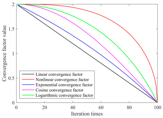
Figure 1.
Comparison of the convergence trends of the convergence factors.
Figure 1 demonstrates that, compared with the linear convergence factor of the traditional GWO algorithm, the other four convergence factors show the convergence trend of the convex function. In the early iteration, the time of the nonlinear convergence factor that is greater than 1 is significantly more than other convergence factors, which helps to enrich the diversity of the grey wolf population and improves the algorithm’s global searchability. At the end of the iteration, the nonlinear convergence factor decreases in an obvious manner, which accelerates the convergence speed of the algorithm.
This paper applies the IGWO algorithm to optimize the SVM parameters. The primary process of optimization is as follows.
- (1)
- Set the initial scale and related parameters of the IGWO algorithm, and initialize the parameters of the SVM model [c, g].
- (2)
- Randomly initialize the parent, mutation, and offspring gray wolf populations, and determine the α, β and δ wolves in the parent grey wolf population.
- (3)
- Update the parent population, generate mutations and offspring grey wolf populations, and perform crossover operations.
- (4)
- Compare the fitness value of the parent population and the offspring variant population. If the offspring population is preferable, replace the parent population fitness value and update the parent population. Otherwise, it should remain unchanged.
- (5)
- Update a′, A, and C according to Formulas (11) and (18).
- (6)
- When the number of iterations reaches the set maximum value, terminate the iteration, and the SVM model’s optimal [c, g] parameter combination will be output. Otherwise, return to step 3 and continue the iteration.
The pseudocode of the IGWO optimization process is shown in Algorithm 1.
| Algorithm 1. The pseudocode of the IGWO optimization process. |
| Initialize n, Itermax, and other parameters, |
| Initialize the location of parent population, mutant population and offspring population, and calculate the corresponding individual target fitness value, |
| Identify α, β, δ wolves in the parent population, |
| [~,sort_index] = sort (parent_wolf); |
| parent_α_Position = parent_Position (sort_index (1), :); |
| parent_α_wolf = parent_wolf (sort_index (1)); |
| parent_β_Position = parent_Position (sort_index (2), :); |
| parent_δ_Position = parent_Position (sort_index (3), :); |
| Fitness = zeros (1, Itermax); |
| Fitness (1) = parent_α_wolf; |
| for t = 1:Itermax |
| Calculate the value of the nonlinear convergence factor according to formula (24); |
| for p = 1:n |
| Update the parent individual location according to Formulas (15)–(21); |
| Calculate the fitness value of the parent individual; |
| end |
| Generate the mutant population according to Formula (22) |
| Generate the offspring population, and perform the crossover operation according to Formula (23); |
| Calculate the fitness value of new offspring; |
| for p = 1:n |
| if offspring_wolf (p) < parent_wolf (p) |
| parent_wolf (p) = offspring_wolf (p) |
| Fitnessbest = parent_wolf (p) |
| end |
| end |
| [~,sort_index] = sort (parent_wolf); |
| parent_α_Position = parent_Position (sort_index (1), :); |
| parent_α_wolf = parent_wolf (sort_index (1)); |
| parent_β_Position = parent_Position (sort_index(2), :); |
| parent_δ_Position = parent_Position (sort_index(3), :); |
| Fitness (t) = parent_α_wolf; |
| end |
| cbest = parent_α_Position (1,1); |
| gbest = parent_α_Position (1,2); |
| Postprocess the results and visualization. |
4. Establishment of the Cutting Pattern Recognition Model
This paper proposes a cutting pattern recognition model based on ICEEMDAN–IGWO–SVM to improve the recognition accuracy of cutting sound signals. It divides the model into sound signal processing, model parameter optimization, and cutting pattern recognition.
- (1)
- Sound signal processing: Aiming at the shearer cutting sound signal, it processes the signal through the ICEEMDAN method and extracts the CMPE of the IMF component as the eigenvalue.
- (2)
- Model parameter optimization: The paper initializes the parameters. Then, it uses the DE algorithm and nonlinear convergence factors to optimize the GWO algorithm and search for the optimal parameter combination of the SVM.
- (3)
- Cutting pattern recognition: The optimal parameter combination determines the SVM model, which can perform cutting pattern recognition research based on the eigenvalues.
The cutting pattern recognition model, based on ICEEMDAN–IGWO–SVM, is shown in Figure 2.
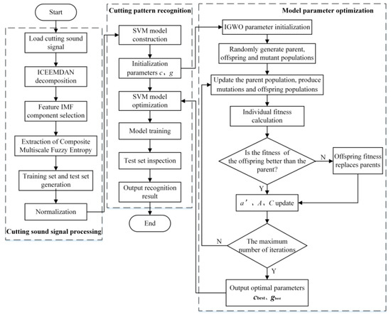
Figure 2.
Flow chart of the cutting pattern recognition model.
5. Experiment and Analysis
5.1. Cutting Sound Signal Acquisition
The experimental data of this paper came from the shearer simulating cutting experimental system made by the research group, as shown in Figure 3.
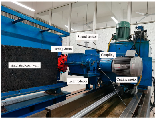
Figure 3.
Shearer simulating cutting experimental system.
The system was based on the MG2X160/710WD thin shearer as the prototype. It took the cutting drum as the research object. Meanwhile, a similarity coefficient of ¼ was applied to develop the system [49]. According to the existing data, the compressive strength of artificial coal samples is about 2.5 times that of natural coal samples. This indicates that a simulated coal sample with a compressive strength of 1MPa is equivalent to a natural coal sample with a compressive strength of 2.5 MPa.
The experiment determined the compressive strength calculation formula between the simulated and natural coal samples.
where σm is the compressive strength of the simulated coal wall, σ represents the compressive strength of the natural coal sample, μ refers to the similarity coefficient, and φ is the strength coefficient.
σm=σ·μ·φ
According to Formula (26), the compressive strength relationship between the simulated coal sample and the natural coal sample in this experimental system was 1/10. This indicates that the simulated coal sample with a compressive strength of 1 MPa was similar to a natural coal sample with a compressive strength of 10 MPa. Thus, the experiment involved the pouring of three simulated coal walls with a length × width × height of 700 mm × 200 mm × 500 mm according to the proportioning scheme. These strengths were 1 MPa, 2 MPa, and 3 MPa, and the corresponding natural coal sample strengths were 10 MPa, 20 MPa, and 30 MPa. Meanwhile, the shearer cut the simulated coal walls of 1 MPa, 2 MPa, and 3 MPa, which were marked as cutting mode 1, cutting mode 2, and cutting mode 3, respectively.
When cutting, the cutting drum forward speed was set to 0.5 m/min. It inputted a frequency of 30 Hz through the inverter so that the cutting motor speed was 858 r/min. The cutting motor was connected with the gear reducer through the coupling and finally drove the cutting drum for rotary cutting. According to the calculation, the cutting drum speed was 111.4 r/min. The cutting effect is reflected in Figure 4.
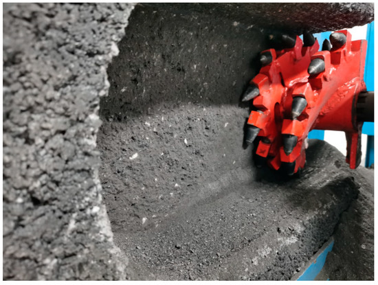
Figure 4.
Shearer cutting experiment.
The pick collided and impacted on the simulated coal sample when the cutting drum runs, producing a cutting sound signal. The experiment used the sound sensor to collect the cutting sound signal and transmit it to the acquisition system. The hardware list of the sound signal acquisition system is listed in Table 1.

Table 1.
Hardware details of the sound signal acquisition system.
The sampling frequency of the cutting sound signal was set to 48KHz, and the number of sampling points was set to 4800. Figure 5 indicates the sound signals of the three cutting modes.
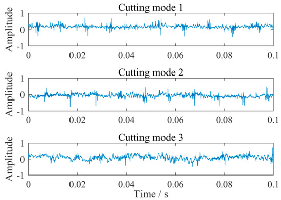
Figure 5.
The waveform of the cutting sound signal.
Figure 5 reflects that the difference in the waveform of the sound signals generated by the three cutting modes was relatively tiny, and it is difficult to distinguish them significantly. Meanwhile, the three cutting sound signals all had obvious non-stationarity. Therefore, this study used the proposed method to process and recognize the cutting sound signal.
5.2. Processing and Feature Extraction of the Cutting Sound Signal
This study took cutting mode 1 as an example and applied the ICEEMDAN method to process the cutting sound signal. The decomposed IMF components are shown in Figure 6.
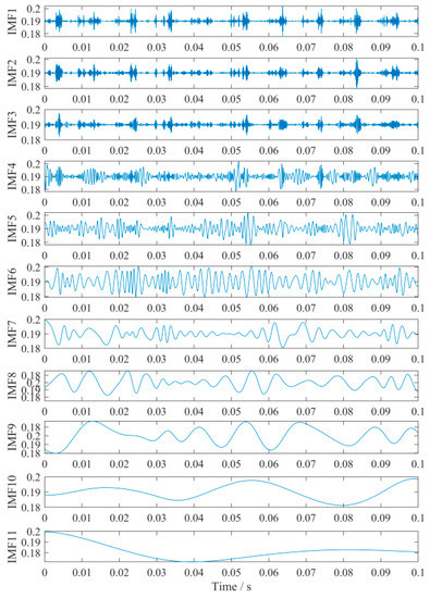
Figure 6.
Decomposition results of the cutting sound signal.
Figure 6 shows that the sound signal of cutting mode 1 was processed to obtain 11 IMF components. In order to select the IMF components that contained the main characteristics of the cutting sound signal, the method calculated the correlation coefficient between the IMF component and the original cutting sound signal. It obtained the correlation coefficients of 11 IMF components, and the results are listed in Table 2.
Table 2.
The correlation coefficient of the IMF component.
Table 2 reflects that the correlation coefficient of IMF5 was the largest, with a value is 0.4616. According to the selection principle of the correlation coefficient, the larger the correlation coefficient of the IMF component, the wealthier the characteristic information. IMF5 had the most significant correlation coefficient and contained the most cutting feature information. Therefore, IMF5 was defined as the characteristic IMF component of the sound signal generated by cutting mode 1. Meanwhile, the sound signals of cutting mode 2 and cutting mode 3 were processed to obtain the corresponding characteristic IMF components. Then, the CMPE of the characteristic IMF component was calculated. Under the three cutting modes, this study obtained 20 sets of sound signals and calculated the mean and standard deviation curves of the CMPE, as shown in Figure 7.
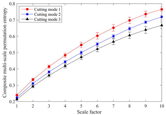
Figure 7.
The mean value and standard deviation curve of composite multi-scale permutation entropy.
Figure 7 shows that as the strength of the simulated coal wall increased, the looseness of the coal sample decreased. This weakened the irregularity of the sound signal generated by the cutting, thereby reducing the CMPE. Moreover, the CMPE of the sound signals of the three cutting modes had the same changing trend with the scale factor. Meanwhile, as the scale factor increased, the difference between entropy values gradually became more considerable. Therefore, it was practical to use the CMPE of the characteristic IMF component as the feature of cutting pattern recognition.
5.3. Cutting Pattern Recognition
The experiment established three cutting modes and collected the sound signals generated during cutting. A total of 200 sets of data were randomly selected for each cut mode. The training set and test set were divided at a ratio of 7:3. Meanwhile, the paper applied the ICEEMDAN method to process the cutting sound signal. It used the correlation coefficient method to select the characteristic IMF component and calculated its CMPE as the characteristic value. Furthermore, this method took the CMPE of the signal as the input of the cutting pattern recognition model based on IGWO–SVM after normalization, and took the shearer cutting pattern as the output.
The parameters of the IGWO–SVM cutting pattern recognition model were set as follows. The grey wolf population size was 20. The maximum number of iterations was 100. Meanwhile, the lower and upper bounds of the scaling factor were 0.2 and 0.8. The crossover probability was set to 0.2. Moreover, the value ranges of the SVM model parameters c and g were both [0.01, 100]. The mean square error was selected as the fitness function of the IGWO–SVM model. When the mean square error value reached the minimum, the target parameter value was close to the optimal value. The optimization curve of the IGWO–SVM model is shown in Figure 8.
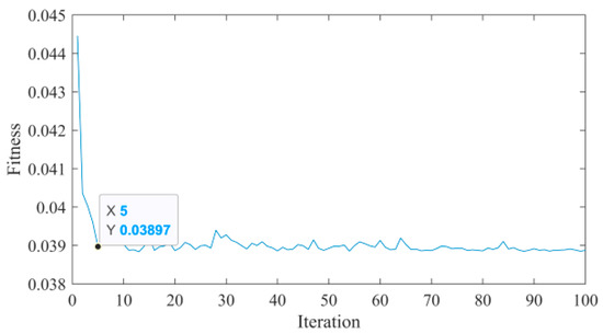
Figure 8.
Fitness optimization curve.
Figure 8 indicates that the IGWO–SVM model tended to converge around the fifth generation. The fitness fluctuated in a small range in the optimization process to avoid the model falling into the local optimum. It could thus be determined that the best parameter combination of c and g was [2.92, 92.06]. Using the optimized parameter IGWO–SVM model for cutting pattern recognition, the recognition accuracy reached 97.78%. The cutting pattern recognition result is shown in Figure 9.
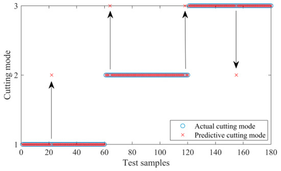
Figure 9.
Cutting pattern recognition results.
In order to verify the performance of the proposed IGWO–SVM model, this study applied ABC, PSO, GWO, and IGWO to optimize the SVM. The initial population size of the four models was set to 20 and the maximum number of iterations was set to 100. The number of honey sources in the ABC algorithm was 10. Meanwhile, the maximum number of searches was 20. Furthermore, the learning factors of the PSO algorithm were 1.5 and 1.6, respectively, and the inertia weights were 0.4 and 0.9. The identification and comparison results of the four models obtained by the ten-fold cross-validation method are listed in Table 3. The accuracy error was the highest accuracy minus the lowest accuracy. Similarly, the time-consuming error was the maximum recognition time − the minimum recognition time.
Table 3.
Performance comparison of four cutting pattern recognition models.
Table 3 shows that using the CMPE as the feature value, the cutting pattern recognition rate of the four models was relatively high. The average recognition rate of the PSO–SVM model was 95.61%, which was the lowest. Meanwhile, the accuracy error was the largest, reaching 3.84%. Furthermore, the average recognition time was 0.74s, which was the highest. The PSO–SVM model had the most unstable performance. The average accuracy of the ABC–SVM and GWO–SVM models was 96.11%. However, the accuracy error of the ABC–SVM model was 3.34%, while that of the GWO–SVM model was 0. The average accuracy of the IGWO–SVM model was the highest, reaching 97.67. Its accuracy error was 0.56%. Meanwhile, the average recognition time and time-consuming error of the IGWO–SVM model were the lowest. The above results show that the IGWO–SVM recognition model proposed in this paper demonstrated excellent performance for shearer cutting pattern recognition.
6. Conclusions
This paper proposed a method of sound signal recognition for shearer cutting based on the ICEEMDAN and IGWO–SVM models. It applied the ICEEMDAN method to process the cutting sound signal of the shearer and extracted the characteristic IMF component through the correlation coefficient. Moreover, the extension of the CMPE model, based on permutation entropy, made it possible to effectively extract the characteristic information of the cutting sound signal, which helped to improve the accuracy of the shearer cutting pattern recognition. The paper established the IGWO–SVM cutting pattern recognition model by introducing the DE algorithm and the nonlinear convergence factor. Furthermore, it improved the global search capability of GWO, avoided the problem of the algorithm falling into the local optimum in the later stage, and promoted the convergence speed at the same time. On this foundation, the cutting experiment was carried out through the simulation cutting experiment system. The average recognition rate of the cutting pattern reached 97.67%, which was better than the commonly used classification and recognition models. Therefore, this method provided a new research idea for precisely recognizing shearer cutting patterns based on cutting sound signals.
However, the method in this paper also had some shortcomings. On the one hand, it did not consider the influence of noise on the experimental results. The underground environments of coal mines are harsh, and the intense noise will affect the accuracy of the cutting sound signal acquisition and analysis. On the other hand, the experiment only analyzed the discrete data and did not recognize the continuous cutting sound signal. Therefore, the authors plan to conduct theoretical analyses and experimental research on sound signal denoising and on-line cutting pattern recognition systems in future research.
Author Contributions
Conceptualization, T.P. and C.L.; methodology, T.P. and C.L.; software, C.L.; validation, T.P., C.L. and Y.Z.; formal analysis, C.L.; resources, T.P.; data curation, C.L.; writing—original draft preparation, C.L.; writing—review and editing, T.P.; project administration, T.P.; funding acquisition, T.P. All authors have read and agreed to the published version of the manuscript.
Funding
This research was funded by the National Natural Science Foundation of China (No. 51475001).
Institutional Review Board Statement
Not applicable.
Informed Consent Statement
Not applicable.
Data Availability Statement
The data present in this study are available on request from the corresponding author.
Conflicts of Interest
The authors declare no conflict of interest.
References
- Chen, X.; Yang, Z.; Cheng, G. Research on coal-rock recognition based on sound signal analysis. MATEC Web Conf. 2018, 232, 04075. [Google Scholar] [CrossRef]
- Bessinger, S.L.; Nelson, M.G. Remnant roof coal thickness measurement with passive gamma ray instruments in coal mines. IEEE Trans. Ind. Appl. 1993, 29, 562–565. [Google Scholar] [CrossRef]
- Kuenzer, C.; Bachmann, M.; Mueller, A.; Lieckfeld, L.; Wagner, W. Partial unmixing as a tool for single surface class detection and time series analysis. Int. J. Remote Sens. 2008, 29, 3233–3255. [Google Scholar] [CrossRef]
- Ralston, J.; Reid, D.; Hargrave, C.; Hainsworth, D. Sensing for advancing mining automation capability: A review of underground automation technology development. Int. J. Min. Sci. Technol. 2014, 24, 305–310. [Google Scholar] [CrossRef]
- Miao, S.; Liu, X. Free Radical Characteristics and Classification of Coals and Rocks Using Electron Spin Resonance Spectroscopy. J. Appl. Spectrosc. 2019, 86, 345–352. [Google Scholar] [CrossRef]
- Si, L.; Wang, Z.-B.; Jiang, G. Fusion Recognition of Shearer Coal-Rock Cutting State Based on Improved RBF Neural Network and D-S Evidence Theory. IEEE Access 2019, 7, 122106–122121. [Google Scholar] [CrossRef]
- Si, L.; Wang, Z.; Liu, X.; Tan, C. A sensing identification method for shearer cutting state based on modified multi-scale fuzzy entropy and support vector machine. Eng. Appl. Artif. Intell. 2019, 78, 86–101. [Google Scholar] [CrossRef]
- Vamsi, I.; Sabareesh, G.; Penumakala, P. Comparison of condition monitoring techniques in assessing fault severity for a wind turbine gearbox under non-stationary loading. Mech. Syst. Signal Process. 2019, 124, 1–20. [Google Scholar] [CrossRef]
- Amarnath, M.; Praveen Krishna, I.R. Local fault detection in helical gears via vibration and acoustic signals using EMD based statistical parameter analysis. Measurement 2014, 58, 154–164. [Google Scholar] [CrossRef]
- Ji, L.; Cheng, D.; Yi, C.; Zick, S. The separation of aircraft background acoustic blindness based on EEMD-ICA. J. Intell. Fuzzy Syst. 2019, 37, 509–516. [Google Scholar] [CrossRef]
- Xu, J.; Wang, Z.; Tan, C.; Si, L.; Zhang, L.; Liu, X. Adaptive Wavelet Threshold Denoising Method for Machinery Sound Based on Improved Fruit Fly Optimization Algorithm. Appl. Sci. 2016, 6, 199. [Google Scholar] [CrossRef] [Green Version]
- Xu, J.; Wang, Z.; Tan, C.; Si, L.; Liu, X. A Novel Denoising Method for an Acoustic-Based System through Empirical Mode Decomposition and an Improved Fruit Fly Optimization Algorithm. Appl. Sci. 2017, 7, 215. [Google Scholar] [CrossRef] [Green Version]
- Huang, H.B.; Li, R.X.; Yang, M.L.; Lim, T.C.; Ding, W.P. Evaluation of vehicle interior sound quality using a continuous restricted Boltzmann machine-based DBN. Mech. Syst. Signal Process. 2017, 84, 245–267. [Google Scholar] [CrossRef] [Green Version]
- Damaševičius, R.; Napoli, C.; Sidekerskienė, T.; Woźniak, M. IMF mode demixing in EMD for jitter analysis. J. Comput. Sci. 2017, 22, 240–252. [Google Scholar] [CrossRef]
- Singh, D.S.; Zhao, Q. Pseudo-fault signal assisted EMD for fault detection and isolation in rotating machines. Mech. Syst. Signal Process. 2016, 81, 202–218. [Google Scholar] [CrossRef]
- Fu, Q.; Jing, B.; He, P.; Si, S.; Wang, Y. Fault Feature Selection and Diagnosis of Rolling Bearings Based on EEMD and Optimized Elman_AdaBoost Algorithm. IEEE Sens. J. 2018, 18, 5024–5034. [Google Scholar] [CrossRef]
- Lu, Y.; Xie, R.; Liang, S.Y. CEEMD-assisted kernel support vector machines for bearing diagnosis. Int. J. Adv. Manuf. Technol. 2020, 106, 3063–3070. [Google Scholar] [CrossRef]
- Li, Y.; Chen, X.; Yu, J. A Hybrid Energy Feature Extraction Approach for Ship-Radiated Noise Based on CEEMDAN Combined with Energy Difference and Energy Entropy. Processes 2019, 7, 69. [Google Scholar] [CrossRef] [Green Version]
- Huang, Y.; Yang, D.; Wang, K.; Wang, L.; Fan, J. A quality diagnosis method of GMAW based on improved empirical mode decomposition and extreme learning machine. J. Manuf. Process. 2020, 54, 120–128. [Google Scholar] [CrossRef]
- Wang, L.; Shao, Y. Fault feature extraction of rotating machinery using a reweighted complete ensemble empirical mode decomposition with adaptive noise and demodulation analysis. Mech. Syst. Signal Process. 2020, 138, 106545. [Google Scholar] [CrossRef]
- Colominas, M.A.; Schlotthauer, G.; Torres, M.E. Improved complete ensemble EMD: A suitable tool for biomedical signal processing. Biomed. Signal Process. Control. 2014, 14, 19–29. [Google Scholar] [CrossRef]
- Deng, X.; Xu, T.; Wang, R. Risk Evaluation Model of Highway Tunnel Portal Construction Based on BP Fuzzy Neural Network. Comput. Intell. Neurosci. 2018, 2018, 8547313. [Google Scholar] [CrossRef] [PubMed] [Green Version]
- Wu, Y.; Zhang, Z.; Li, Y.; Sun, Q. Open-circuit fault diagnosis of six-phase permanent magnet synchronous motor drive system based on empirical mode decomposition energy entropy. IEEE Access 2021, 9, 91137–91147. [Google Scholar] [CrossRef]
- Chen, Q.-Q.; Dai, S.-W.; Dai, H.-D. A Rolling Bearing Fault Diagnosis Method Based on EMD and Quantile Permutation Entropy. Math. Probl. Eng. 2019, 2019, 3089417. [Google Scholar] [CrossRef] [Green Version]
- Si, L.; Wang, Z.; Tan, C.; Liu, X.; Xu, X. A Feature Extraction Method for Shearer Cutting Pattern Recognition Based on Improved Local Mean Decomposition and Multi-Scale Fuzzy Entropy. Curr. Sci. 2017, 112, 2243. [Google Scholar] [CrossRef]
- Costa, M.; Goldberger, A.L.; Peng, C.-K. Multiscale Entropy Analysis of Complex Physiologic Time Series. Phys. Rev. Lett. 2002, 89, 068102. [Google Scholar] [CrossRef] [Green Version]
- Costa, M.; Goldberger, A.L.; Peng, C.-K. Multiscale entropy analysis of biological signals. Phys. Rev. E 2005, 71, 021906. [Google Scholar] [CrossRef] [Green Version]
- Jia, R.-S.; Sun, H.-M.; Peng, Y.-J.; Liang, Y.-Q.; Lu, X.-M. Automatic event detection in low SNR microseismic signals based on multi-scale permutation entropy and a support vector machine. J. Seism. 2016, 21, 735–748. [Google Scholar] [CrossRef]
- Dong, Z.; Zheng, J.; Huang, S.; Pan, H.; Liu, Q. Time-Shift Multi-scale Weighted Permutation Entropy and GWO-SVM Based Fault Diagnosis Approach for Rolling Bearing. Entropy 2019, 21, 621. [Google Scholar] [CrossRef] [Green Version]
- Xu, F.; Tse, P.W.T.; Fang, Y.-J.; Liang, J.-Q. A fault diagnosis method combined with compound multiscale permutation entropy and particle swarm optimization–support vector machine for roller bearings diagnosis. Proc. Inst. Mech. Eng. Part J J. Eng. Tribol. 2019, 233, 615–627. [Google Scholar] [CrossRef]
- Xie, X.; Chen, W.; Chen, B.; Cheng, J.; Tan, L. Comprehensive fatigue estimation and fault diagnosis based on Refined Generalized Multi-Scale Entropy method of centrifugal fan blades. Measurement 2020, 166, 108224. [Google Scholar] [CrossRef]
- Dou, D.; Qiu, Z.; Yang, J. Parameter optimization of an industrial water injection hydrocyclone in the Taixi coal preparation plant. Int. J. Coal Prep. Util. 2020, 1–9. [Google Scholar] [CrossRef]
- Gupta, S.; Deep, K. Random walk grey wolf optimizer for constrained engineering optimization problems. Comput. Intell. 2018, 34, 1025–1045. [Google Scholar] [CrossRef]
- Tan, X.; Yu, F.; Zhao, X. Support vector machine algorithm for artificial intelligence optimization. Clust. Comput. 2019, 22, 15015–15021. [Google Scholar] [CrossRef]
- Tao, Z.; Huiling, L.; Wenwen, W.; Xia, Y. GA-SVM based feature selection and parameter optimization in hospitalization expense modeling. Appl. Soft Comput. 2019, 75, 323–332. [Google Scholar] [CrossRef]
- Lu, J.; Liao, X.; Li, S.; Ouyang, H.; Chen, K.; Huang, B. An Effective ABC-SVM Approach for Surface Roughness Prediction in Manufacturing Processes. Complexity 2019, 2019, 3094670. [Google Scholar] [CrossRef] [Green Version]
- Mirjalili, S.; Mirjalili, S.M.; Lewis, A. Grey Wolf Optimizer. Adv. Eng. Softw. 2014, 69, 46–61. [Google Scholar] [CrossRef] [Green Version]
- Gupta, S.; Deep, K. Enhanced leadership-inspired grey wolf optimizer for global optimization problems. Eng. Comput. 2019, 36, 1777–1800. [Google Scholar] [CrossRef]
- Torres, M.E.; Colominas, M.A.; Schlotthauer, G.; Flandrin, P. A complete ensemble empirical mode decomposition with adaptive noise. In Proceedings of the 2011 IEEE International Conference on Acoustics, Speech and Signal Processing (ICASSP), Prague, Czech Republic, 22–27 May 2011; pp. 4144–4147. [Google Scholar] [CrossRef]
- Chaabi, L.; Lemzadmi, A.; Djebala, A.; Bouhalais, M.L.; Ouelaa, N. Fault diagnosis of rolling bearings in non-stationary running conditions using improved CEEMDAN and multivariate denoising based on wavelet and principal component analyses. Int. J. Adv. Manuf. Technol. 2020, 107, 3859–3873. [Google Scholar] [CrossRef]
- Ali, M.; Prasad, R. Significant wave height forecasting via an extreme learning machine model integrated with improved complete ensemble empirical mode decomposition. Renew. Sustain. Energy Rev. 2019, 104, 281–295. [Google Scholar] [CrossRef]
- Guo, R.; Zhao, Z.; Wang, T.; Liu, G.; Zhao, J.; Gao, D. Degradation State Recognition of Piston Pump Based on ICEEMDAN and XGBoost. Appl. Sci. 2020, 10, 6593. [Google Scholar] [CrossRef]
- Zhang, X.; Miao, Q.; Zhang, H.; Wang, L. A parameter-adaptive VMD method based on grasshopper optimization algorithm to analyze vibration signals from rotating machinery. Mech. Syst. Signal Process. 2018, 108, 58–72. [Google Scholar] [CrossRef]
- Xiao, R.; Hu, Q.; Li, J. Leak detection of gas pipelines using acoustic signals based on wavelet transform and Support Vector Machine. Measurement 2019, 146, 479–489. [Google Scholar] [CrossRef]
- Miao, D.; Hossain, S. Improved gray wolf optimization algorithm for solving placement and sizing of electrical energy storage system in micro-grids. ISAT 2020, 102, 376–387. [Google Scholar] [CrossRef] [PubMed]
- Al-Betar, M.A.; Awadallah, M.A.; Faris, H.; Aljarah, I.; Hammouri, A.I. Natural selection methods for Grey Wolf Optimizer. Expert Syst. Appl. 2018, 113, 481–498. [Google Scholar] [CrossRef]
- Singh, N.; Singh, S. A novel hybrid GWO-SCA approach for optimization problems. Eng. Sci. Technol. Int. J. 2017, 20, 1586–1601. [Google Scholar] [CrossRef]
- Zhang, X.; Zhang, Y.; Ming, Z. Improved dynamic grey wolf optimizer. Front. Inf. Technol. Electron. Eng. 2021, 22, 877–890. [Google Scholar] [CrossRef]
- Peng, T.; Li, C.; Zhu, Y. Design and Application of Simulating Cutting Experiment System for Drum Shearer. Appl. Sci. 2021, 11, 5917. [Google Scholar] [CrossRef]
Publisher’s Note: MDPI stays neutral with regard to jurisdictional claims in published maps and institutional affiliations. |
© 2021 by the authors. Licensee MDPI, Basel, Switzerland. This article is an open access article distributed under the terms and conditions of the Creative Commons Attribution (CC BY) license (https://creativecommons.org/licenses/by/4.0/).