A Compact Wideband Active Two-Dipole HF Phased Array

Abstract

The design and construction of an upgraded HF quarter-wavelength two-dipole active array with 90° difference feed was implemented in the course of a research project to perform a directional (azimuthal) investigation of interference at HF. The lack of affordable compact antennas to meet the project requirements was the incentive to develop a compact unidirectional antenna, with the maximum possible front-to-back ratio at frequencies of 20–30 MHz, where the dimensions of traditional passive antennas are enormous. By installing a low-noise very-high-input impedance amplifier in each dipole of the array, the effect of the mutual coupling between the two dipoles was reduced, improving the front-to-back (F/B) ratio over a wide frequency range. Electronic steering, easy polarization adjustment, and fast and easy deployment were the key requirements for the construction of the antenna. Therefore, a light and compact design was of the utmost importance to meet the space limitations at the monitoring site, which did not allow the deployment of a traditional HF directional antenna that employs a very long boom and elements.

1. Introduction

In the context of radio-interference mitigation in the HF spectrum, it is important to monitor HF spectral occupancy characteristics on a systematic basis, which can facilitate the development of relevant prediction models [1,2,3]. In the course of a research project to characterize the HF interference environment over the eastern Mediterranean region, the design and development of phased arrays, in the form of HF quarter-wavelength two-dipole active phased-array antennas with 90° phase difference feeds, was undertaken in an effort to incorporate an azimuthal dimension in the existing measurement system [4]. The phased arrays have been developed and optimized under certain specification requirements, such as limited array size, and the demand for electronic rotation capability. The drawbacks and weaknesses of other traditional arrays’ performance, derived from literature review and antenna design principles, have been considered. For example, two very widely used configurations, Yagi-Uda and log-periodic directional antennas, are usually considered for directional monitoring in HF [3]. The log periodic is an excellent broadband antenna that is traditionally used for monitoring HF signals. It is constituted by end-fire half-wave resonance dipoles, installed side by side at the proper distance along a boom. To operate across the entire HF band with low VSWR, many dipoles installed on a heavy long structure are required [4]. Therefore, an HF log-periodic antenna must be installed on a very stable mast. Furthermore, a heavy-duty rotator is required for steering. Another popular HF monitor antenna is the Yagi-Uda, but with a narrower band response compared to the log periodic [5]. Even a multiband Yagi-Uda antenna that employs traps to operate in several wavelengths across the HF band has a much inferior VSWR response than the log-periodic antenna. The Yagi-Uda antenna’s mechanical specifications are also characterized by their long boom and very heavy structures. On the other hand, phased arrays can be constructed more compactly than the Yagi-Uda and log-periodic antennas because they consist of driven elements whose phase difference does not depend on their size. For example, the passive phased array, which is very widely used in the HF and in other bands, is a quarter-wavelength two-vertical-monopole array, with a 90° phase difference feed [5,6,7]. This array can produce a directional pattern with a very high F/B ratio but only under certain conditions. For instance, constructing the array without taking into account the effect of mutual coupling between the two driven elements produces an array radiation pattern in real conditions quite different from the simulated one based on Equation (6) below [5]. This occurs because the mutual coupling disturbs the phase difference between the two driven elements as well as their current balance, as it is discussed later. A traditional method to compensate for the effect of mutual coupling, but only at a certain frequency of operation, is to adjust the phasing of the array’s elements by lumped-element phase shifters or delay lines. Another approach is to fine tune both driven elements to a 50 Ω purely resistive impedance to ensure 0° phase shift between the voltage and current. Furthermore, the current magnitudes can be balanced by adjusting the length and the distance between the two driven elements [8,9,10]. For all these reasons, a passive phased array is not suitable for broadband operation and radiation patterns, as simulated in ideal conditions and discussed in the next chapter. For an F/B ratio broadband response, the phase difference and the current balance of the two driven elements of the array should be kept as undisturbed as possible throughout the entire frequency operating range. This has been implemented by the use of a very-high-input-impedance, two-stage, low-noise amplifier, which has been installed in each of the two driven elements of the array. The innovative aspect of this approach centres on the mutual coupling isolation that enables a compact array to operate over a wide range with a high sensitivity and F/B ratio. This linear directional antenna is very compact and light and does not require a boom. It can be programmed to steer at the desired direction by the use of a traditional relay switch. The array can be installed in a vertical or horizontal configuration as it employs elements with short size dimensions. Therefore, this HF active phased array has been designed and developed for monitoring sites that do not allow the deployment of a traditional HF directional antenna with a very long boom and elements. In Section 2, we discuss the underlying principles of the phased array; in Section 3, we provide information on specific design considerations and provide preliminary testing results; and in Section 4, we conclude the paper.

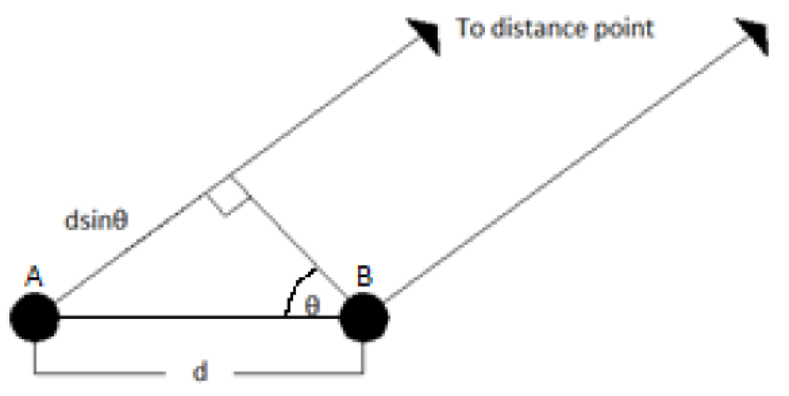
2. Theoretical Model of the Antenna Array

Without minimizing the mutual coupling between the two driven elements of a traditional quarter wavelength phased array with 90° phase difference feed may cause a serious deviation from the expected specifications. For the aforementioned, this fact is manifested in the different simulated and real radiation patterns as discussed below. It can be demonstrated by modelling the array first in ideal conditions by assuming that both driven elements maintain a 50 Ω constant impedance across the entire band, as illustrated in the equivalent circuit in Figure 1. The two driven elements of the array are denoted by the two equal unity voltage sources V1 and V2, both of which have a 50 Ω purely resistive impedance. Furthermore, both antennas are connected to a 90° hybrid that employs three ports of a 50 Ω purely resistive impedance and acts as a beamformer.

At the input ports of the hybrid illustrated in Figure 1, V1 and V2 can then be expressed by Equation (1), where A is the sum of their voltages at the output of the 90° hybrid:

$$A=\sqrt{{\left(1+cos90\right)}^2+{\left(sin0+sin90\right)}^2}=\sqrt{2}$$

(1)

The current magnitudes I₁ and I₂ can be computed by the use of Kirchhoff’s law, where R1 and R2 are the 50 Ω output impedance of each driven element that is terminated at the 50 Ω input ports of the combiner, as given by Equations (2) and (3) below:

V1 = I₁ (R1 + 50)

(2)

V2 = I₂ (R2 + 50)

(3)

Since currents I₁ and I₂ are of identical magnitude, the radiation pattern of the array (assuming that the two driven elements are isotropic radiators) can be plotted by adding vectors using Equations (4) and (5), which have been derived from Figure 2 as follows:

$$\mathsf{\Psi }=\frac{\pi }{2}sin\theta +\mathsf{\Delta }\mathsf{\Phi }$$

(4)

$$AF=\sqrt{{\left(1+cos\psi \right)}^2+{\left(sin\psi \right)}^2}$$

(5)

where:

• AF = Array factor
• θ = The radiation angle
• d = $\frac{\pi }{2}$
• ΔΦ = The phase difference feed

According to Kraus [10], the normalized value of the total field of two isotropic sources referred to as the ‘array factor’ can also be expressed by Equation (6) as follows [6]:

$$\mathrm{E}=\frac{sin\left(2\psi /2\right)}{2sin\left(\psi /2\right)}$$

(6)

Under the condition that both driven elements have a 50 Ω purely resistive impedance and a constant 90° phase difference feed across the desired band, the only parameter that affects the array’s radiation pattern, based on the above given equations, is the element’s spacing because varies according to the wavelength which the antenna is tuned. It is illustrated in Figure 3, where the radiation patterns of two isotropic sources spaced from 0.05 λ to 0.5 λ with a 90° phase difference feed have been simulated. The radiation patterns below have been simulated at different wavelengths using Equations (4) and (5) in order to determine the range at which the array has a usable F/B. In this regard, the mutual coupling between the two elements of the array has not been considered as it affects the active impedance of the array’s driven elements and consequently the array factor, as discussed in the next section.

It is important to note that the value of the self-impedance of an isolated driven element changes under the following conditions. Particularly, according to Balanis, it is defined as the active impedance when two driven elements which are excited installed side by side as a phased array [11,12,13,14]. The mutual resistance and reactance for the case of two parallel, side-by-side antennas, as a function of spacing, was also demonstrated by Kraus. It is based on the integral equation method presented by King and Harrison and by Tai [15]. For the aforementioned, the effect of the mutual coupling on the radiation pattern between two parallel driven elements is modelled in Figure 4. Two isolated driven elements with 50 Ω purely resistive impedance, installed as a phased array, now exhibit an active impedance of 35 − j20 Ω and 65 + j20 Ω, respectively. In this case, both dipoles are in phase and terminated at the 50 Ω 0° combiner input ports. The reason for a 0° instead of 90° hybrid combiner is due to the phase error that is more evident on the oscilloscope screen.

Based on Figure 4, the phasing error and the current imbalance can be calculated by the use of Equations (7) and (8):

$${\mathrm{I}}_1=\frac{\mathrm{V}1}{85-\mathrm{j}20}{\mathsf{\Theta }}_1={\mathrm{Tan}}^{-1}\frac{20}{\left(85\right)}$$

(7)

$${\mathrm{I}}_2=\frac{\mathrm{V}2}{115+\mathrm{j}20}\mathsf{\Theta }{2}_{}={\mathrm{Tan}}^{-1}\frac{20}{\left(115\right)}$$

(8)

The simulation results are demonstrated in Figure 5 as computed at the input ports of the combiner. The first two waveforms, at the top, present the voltages at the input ports of the 50 Ω combiner. Based on Figure 5, a current imbalance and a small phase shift occurs between the first two waveforms. This is caused by the coupling between the two driven elements of the array. The other two waveforms at the bottom of Figure 5 demonstrate the two driven elements when terminated into a very high input impedance port; therefore, no phase error and current imbalance occurs.

The impact of the above is presented in Figure 6 by applying the current values and phase shift in Equation (5). The brown color cardioid radiation pattern reflects ideal conditions. The mutual coupling between the two driven elements of the array affects the radiation pattern as presented by the blue color diagram. It has a small back lobe and a slightly different form. As a result, if the current imbalance and phase error goes far beyond ideal values, then the radiation pattern of the array is expected to be less directional and the F/B ratio will decrease.

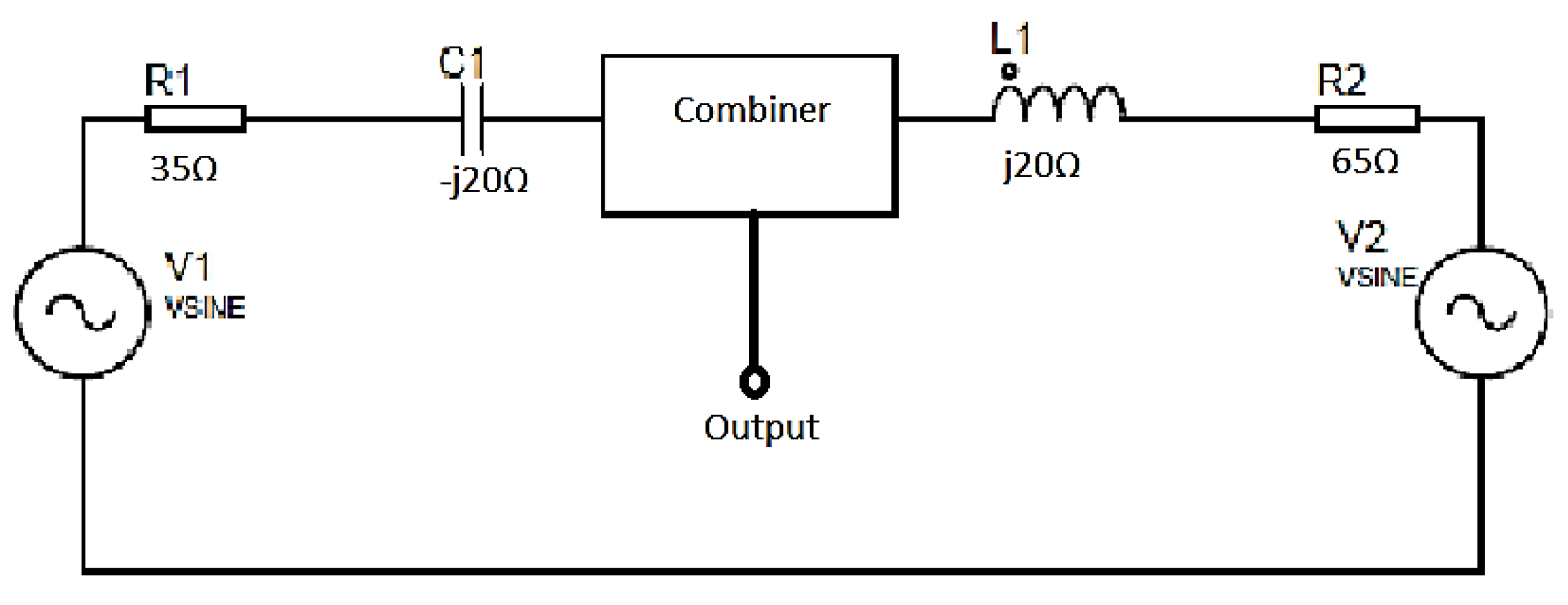
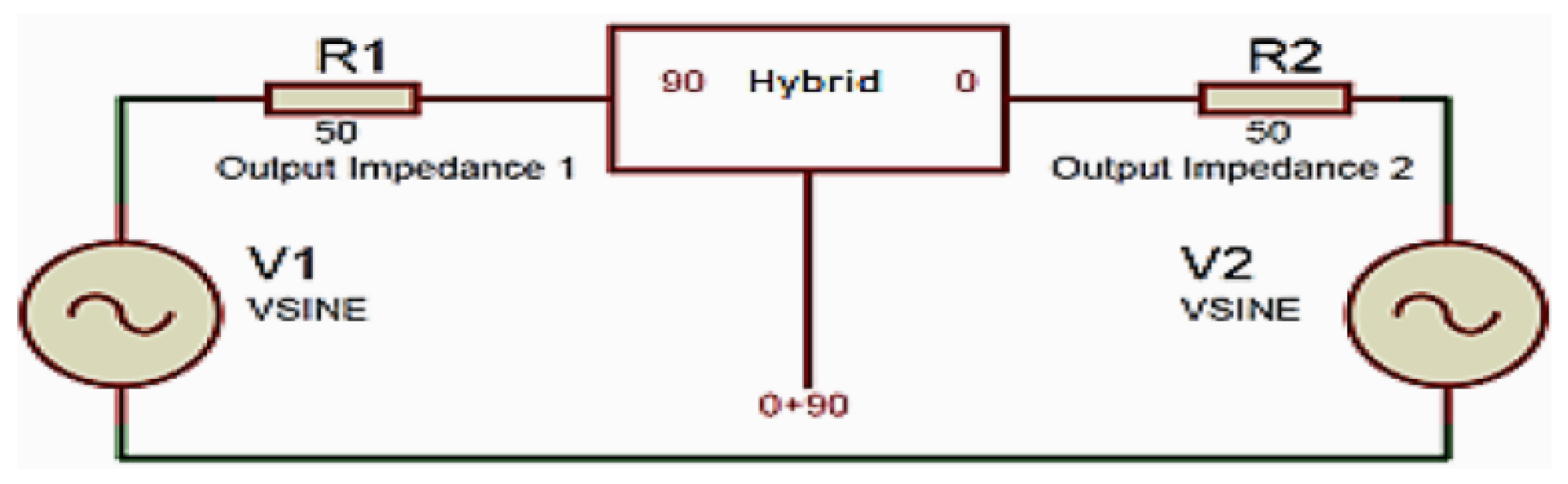
3. Design Considerations

The aim was to construct a two-dipole phased array, employing elements that are as short as possible in order to be easily installed at the desired polarization sense. A good trade-off was to set the length of the dipole elements at 5 m, i.e., 2.5 m for each element with an 8 mm tubing diameter. As a result, both dipoles are short in the lower HF band but close to resonance at 30 MHz. The self-impedances of the short dipoles and the E-plane half-power beam widths (HPBWs) have been simulated from 5 to 30 MHz and are depicted in

Table 1. Free space impedance of the array’s driven elements and HPBW as simulated by Eznec.

Impedance (Ω)	Freq. (MHz)	E-Plane HPBW (Degrees)
80 + j43	30	77
53 − j160	25	81
32 − j412	20	84
17 − j764	15	86
7 − j1374	10	88
1.9 − j3016	5	90

below:

The phase errors and current imbalance of the quarter-wavelength two-dipole phased array is neither easy to calculate nor is it a standard design parameter. Therefore, there is no point in presenting charts and equations that concern the calculation of the mutual coupling between the two parallel dipoles. The aforementioned is affected by many complicated factors such as the operating environment, the height above the ground, the type of ground, the polarization sense of the dipoles, the distance between them, etc. That is why the isolation of the two dipoles, to avoid a current imbalance and phase error, must be maximized as much as possible. Since the two dipoles are installed side by side, the active impedance of each driven element due to the effect of mutual coupling will be different, as has been discussed previously by Kraus [15]. The active dipoles terminated at a 50 Ω combiner should enable balance of the impedance variations, as expressed by the following equations:

$$\mathsf{\Theta }={\mathrm{Tan}}^{-1}\frac{X}{\left(R+50\right)}$$

(9)

$$I=\frac{V}{{[{\left(R+50\right)}^2+{\left(X\right)}^2]}^{0.5}}$$

(10)

where:

• I is the current at the input port of the hybrid,
• V is the output voltage of the active antenna,
• Θ is the phase angle in degrees,
• R is the real part of the antenna’s active impedance, and
• X is the imaginary part of the antenna’s active impedance.

For this to be accomplished, a two-stage LNA has been implemented, as shown in Figure 7. The first stage of the amplifier has been designed around the JFET BF245B as a common drain amplifier [16]. The advantage of this unity voltage-gain, low-noise amplifier is that it presents a very-high-input impedance and a low-noise figure across the HF band, which is about 1.5 dB. Based on Equations (7) and (8), the high-input-impedance property of the JFET amplifier serves two fundamental purposes: it reduces losses from the effect of the short dipole’s high reactive components, given in Table 1; and, on the other hand, isolates the two dipoles in terms of mutual impedance variations. The role of the second stage, class A small-signal common-emitter amplifier is to compensate for the unity voltage gain of the JFET amplifier and also to match the dipole’s terminal impedance at the 50 Ω hybrid’s input port. The performance of the LNA has been evaluated with a response given in Figure 8. The amplifier gain response is not flat due to the Miller effect, mainly on the second stage of the LNA, as was expected, but can be corrected, if needed, by the use of a simple high-pass filter at the output of the combiner. The input impedance of the BF 245B at 25 MHz has been measured to be around 800 Ω using an oscilloscope and the voltage divider method. Specifically, a variable resistor (4K7) was placed in series to a 50 Ω signal generator‘s output. Initially, the probe of the oscilloscope was connected at the output of the signal generator without a load in order to determine the open circuit voltage. The next step was to connect the signal generator at the input of the BF 245 common drain amplifier. The probe of the oscilloscope was connected at the input of BF 245B as well. The target was to adjust the variable resistor, which was in series, with the signal generator output to obtain the half voltage level compared to the open circuit’s voltage measured initially. The resistance value of the trimmer (input impedance of the BF 245 common drain amplifier) was 800 Ω.

The isolation performance between the two active driven elements has been simulated as follows: a case where the driven element A has an active impedance of 30 − j85 Ω and the driven element B an active impedance of 150 + j65 Ω respectively was examined. The simulation results regarding the phase error and amplitude imbalance are presented in Figure 9. The first two waveforms at the top represent the two driven elements A and B tested by employing a 50 Ω impedance LNA. As can be observed, the phase error and amplitude imbalance are much higher than the other two waveforms at the bottom. The two waveforms at the bottom correspond to the same active dipoles under test but when a high impedance LNA (Figure 7) was used. The phase and amplitude errors significantly reduced due to the very high input impedance of the JFET. The gain of the LNA has not been considered.

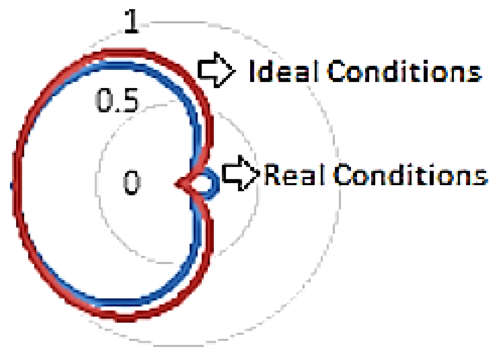
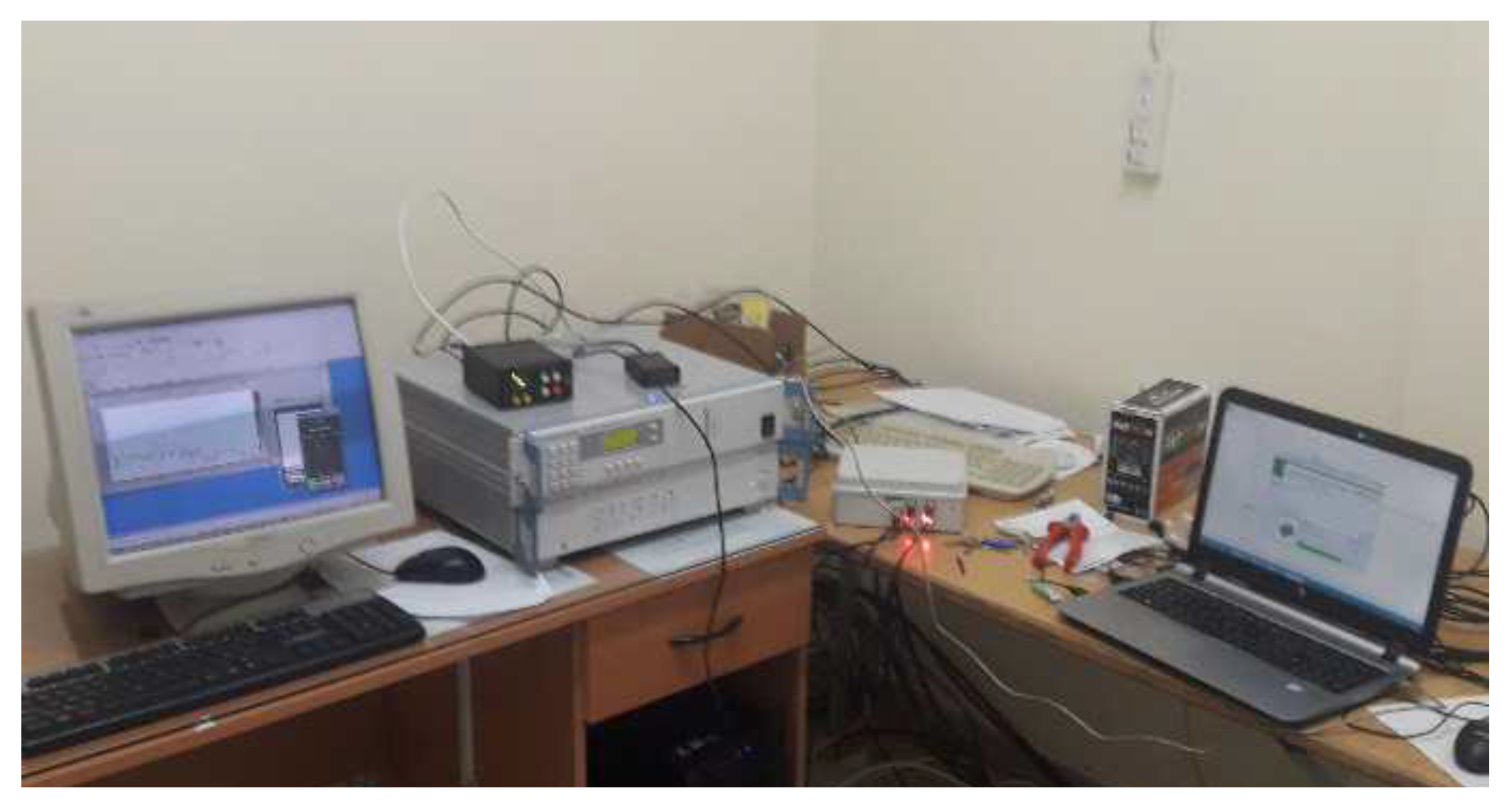
3.1. Preliminary Testing in a Reflection-Free Environment

Preliminary tests before installing the array at the final site have been carried out in real conditions in a reflection-free environment as illustrated in Figure 10. The main focus of the test was to verify the performance difference between an HF quarter-wavelength two-dipole array with 90° difference feed with a high-impedance LNA (presented in Figure 7) versus the identical array with a traditional 50 Ω input-impedance LNA [17]. The array has not been tested utilizing passive dipoles because of their narrow band response in terms of VSWR i.e., it would be required fine tune to 50Ω of each driven element in every frequency under test. A mini-circuit amplifier MAR-8+ has been chosen instead in order to ensure a robust 50 Ω impedance across the spectrum at which the active dipoles are operated. The height of the masts used was 0.33 λ, i.e., not an ideal height at 25 MHz. The length of the dipoles used was 5 m. In order to ensure a broadband 90° phase shift, each dipole was connected at the input port of the Minicircuits broadband splitter/combiner PSCQ-2-51W+ [18]. Using a relay switch presented in Figure 11, the 90° and 0° input ports of the hybrid were reversed.

The chart in Figure 12 presents the response of the F/B ratio with a 50 Ω input-impedance MAR-8+ LNA in each dipole compared to the high-impedance LNA of Figure 7. To implement the test properly, a 30 dBm HF transmitter was installed in the far field, i.e., 1.5 Km away from the reception point that was connected to a half-wave-dipole antenna. For practical reasons, the tested array’s dipoles were installed on a separate mast.

From the preliminary measurements, it is obvious that the array F/B ratio is enhanced when the high-input-impedance LNAs (Figure 7) are used in the two dipoles. Specifically, the array provides a maximum F/B of 26 dB and an average of 19 dB across 18–30 MHz. In contrast, using the 50 Ω Mar-8+ LNA, the array provides a maximum F/B of 17 dB and an average of 12 dB within the same spectrum, as illustrated in Figure 12.

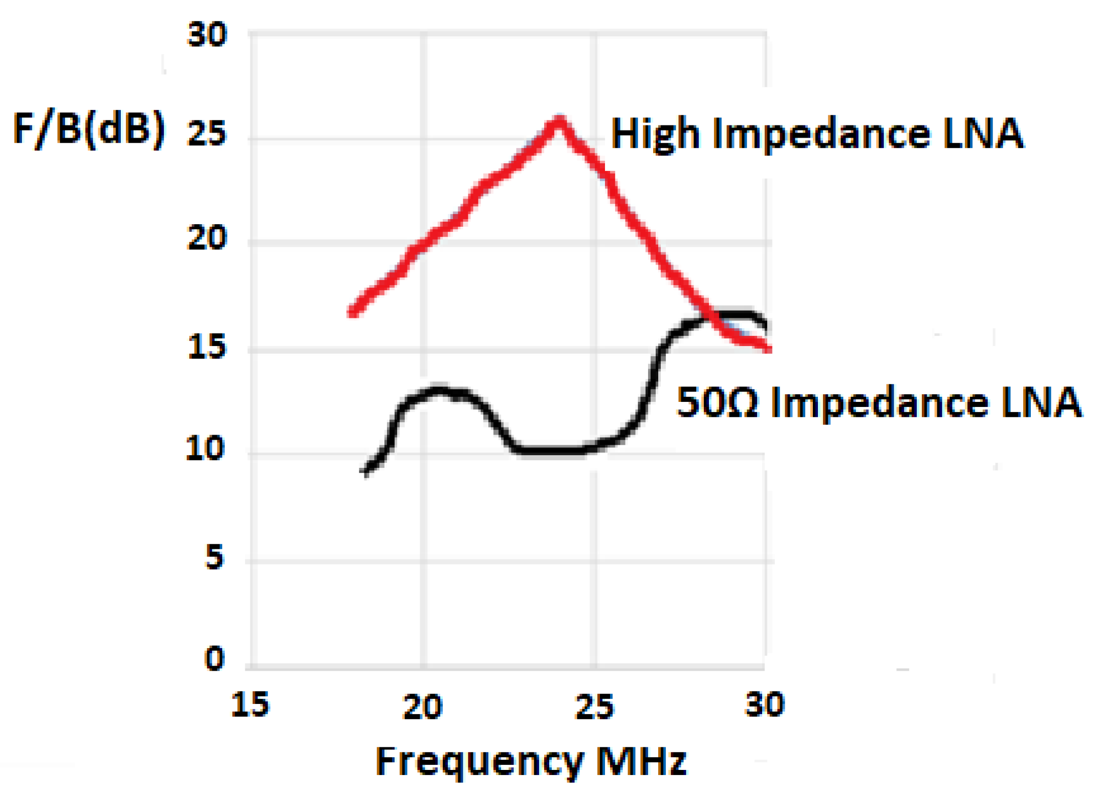
3.2. Final Validation Using Other Antennas

To validate the HF two-dipole active array antenna, we used a Rohde & Schwarz (R&S) EM510 HF digital wideband receiver and dual polarization (HE016) active antenna already installed at the validation site [19]. Since the developed array is horizontally polarized, the omnidirectional turnstile component of the R&S HE016 antenna, capable of receiving HF signals at high incident angles, was used.

Since the dipoles are placed 90° apart, the physical distance between the two dipoles that constitute the antenna at 25 MHz is only 3 m as is illustrated in Figure 13 where the two-dipole phased array is in its final form. The phased antenna steers to the desired direction by the use of an electronic switch that can be controlled by a dedicated software. The HF scans were obtained by the use of an R&S EM510 receiver and an R&S ZS129 hardware switch controlled by ARGUS software [20,21] illustrated in Figure 14 below.

Figure 15 presents the free-space azimuthal response for the quarter-wavelength two horizontal 0.41 λ length dipole phased-array antenna at 25 MHz and 30° elevation angle, as has been simulated by EZNEC based on pattern multiplication principle i.e., beyond the array factor, the array’s radiation pattern is based on the dipoles’ pattern as well. In comparison to Figure 6, the pattern of the 0.25 λ array which was simulated employing isotropic radiators showing HPBW 180° and a 3 dB gain. However, the pattern in Figure 15 showing a HPBW 44.5° and a 7.23 dBi gain. Furthermore, taking advantage of the HE016 antenna which was used as a reference, the sensitivity of the array was evaluated. The phased antenna directions under test were East–West and North–South as illustrated in Figure 16 where the dipole phased-array system is deployed. The results are given in Figure 17 and Figure 18. The scope of this test was to ensure that the active dipoles enabled a good reception below 20 MHz.

It is evident that the proposed array presents a very good performance in terms of receiving signals across the entire HF band, as illustrated in Figure 17. Therefore, the array can be used as a monitor unidirectional antenna for applications below 20 MHz by adjusting the distance between the two dipoles.

The results of testing the front–back ratio of the array between 20 and 30 MHz are given in Figure 18. These results indicate that the array provides a very good F/B ratio between 20 and 30 MHz for air signals, as clearly some of the received signals are suppressed when the array is electronically steered. For instance, based on Figure 18, the F/B ratio is almost 20 dB at 30 MHz as indicated by charts (b) North–South and (d) South–North. The F/B is also of the order of almost 20 dB between 24 and 28 MHz as indicated by charts (a) East–West, and (b) North–South. Between 20 and 24 MHz, signals are also suppressed by switching the arrays in the opposite direction.

4. Concluding Remarks

The design and construction of an upgraded HF quarter-wavelength two-dipole active array with 90° difference feed has been implemented. A high-input-impedance LNA was used in each dipole in order to minimize the mutual coupling effect. Based on the preliminary measurements presented here, it has been demonstrated that the array is operating satisfactorily, providing a respectable F/B ratio between 18 and 30 MHz, ranging from a maximum value of 26 dB to a minimum of 15 dB. An identical array utilizing a 50 Ω LNA that operates in the same spectrum provided a maximum F/B ratio of 16 dB and a minimum of 8 dB. The array steers in four different directions by the use of a computer-controlled relay switch which reverses the hybrid’s input ports in order to steer the array in the opposite direction. The proposed concept will have applications in HF multi-element phased arrays implemented especially for sites where limited space imposes restrictions but where a high directional monitoring antenna is required.

References

1. Economou, L.; Haralambous, H.; Pantjairos, C.; Green, P.; Gott, G.; Laycock, P.; Broms, M.; Boberg, S. Models of HF spectral occupancy over a sunspot cycle. IEE Proc. Commun. 2005, 6, 980–988. [Google Scholar] [CrossRef]
2. Haralambous, H.; Papadopoulos, H. 24-h HF Spectral Occupancy Characteristics and Neural Network Modeling Over Northern Europe. IEEE Trans. Electromagn. Compat. 2009, 59, 1817–1825. [Google Scholar] [CrossRef]
3. Haralambous, H.; Papadopoulos, H. 24-Hour neural network congestion models for high-frequency broadcast users. IEEE Trans. Broadcast. 2017, 55, 145–154. [Google Scholar] [CrossRef]
4. Mostafa, M.G.; Tsolaki, E.; Haralambous, H. HF spectral occupancy time series models over the eastern Mediterranean region. IEEE Trans. Electromagn. Compat. 2016, 59, 240–248. [Google Scholar] [CrossRef]
5. Taguchi, M.; Era, K.; Tanaka, K. Two element phased array dipole antenna. ACES J. 2007, 22, 112–116. [Google Scholar]
6. Bingeman, G. Phased Array Adjustment for Ham Radio. Available online: https://ftp.unpad.ac.id/orari/library/library-sw-hw/amateur-radio/ant/phaseshift/array.htm (accessed on 31 July 2021).
7. Tomas, H. 2m Phased Vertical Antenna. Issuu. 2021. Available online: https://issuu.com/jw9w2ws/docs/2meterphasedvertant (accessed on 31 July 2021).
8. Straw, R. The ARRL Antenna Book; ARRL: Newington, CT, USA, 2009. [Google Scholar]
9. Balanis, C. Antenna Theory; Wiley: Hoboken, NJ, USA, 2016. [Google Scholar]
10. Kraus, J.; Marhefka, R.; Khan, A. Antennas and Wave Propagation; McGraw-Hill: New Delhi, India, 2002. [Google Scholar]
11. Von Aulock, W. Properties of Phased Arrays. Proc. IRE 1960, 48, 1715–1727. [Google Scholar] [CrossRef]
12. Constantinides, A. Collinear Arrays, 1st ed.; ARRL Antenna Compendium: Newington, CT, USA, 2002; Volume 7, pp. 37–39. [Google Scholar]
13. Katagi, T.; Ohmine, H.; Miyashita, H.; Nishimoto, K. Analysis of Mutual Coupling Between Dipole Antennas Using Simultaneous Integral Equations With Exact Kernels and Finite Gap Feeds. IEEE Trans. Antennas Propag. 2016, 64, 1979–1984. [Google Scholar] [CrossRef]
14. Balanis, C. Antenna Theory-Analysis and Design, 3rd ed.; Wiley: Hoboken, NJ, USA, 2005; pp. 479–481. [Google Scholar]
15. Kraus, J. Antennas, 2nd ed.; Mcgraw-Hill: New York, NY, USA, 1988; pp. 424–426. [Google Scholar]
16. Nxp.com. 2021. Available online: https://www.nxp.com/docs/en/data-sheet/BF245A-B-C.pdf (accessed on 30 July 2021).
17. Minicircuits.com. 2021. Available online: https://www.minicircuits.com/pdfs/MAR-8A.pdf (accessed on 30 July 2021).
18. Minicircuits.com. Mini-Circuits. 2021. Available online: https://www.minicircuits.com/WebStore/modelSearch.html?model=PSCQ-2-51W%2B (accessed on 30 July 2021).
19. HE016 | Brochure and Datasheet. Rohde-Schwarz.com. 2021. Available online: https://www.rohde-schwarz.com/brochure-datasheet/he016/ (accessed on 30 July 2021).
20. Manualslib.com. R&S EM510 Manual Pdf Download | ManualsLib. 2021. Available online: https://www.manualslib.com/manual/1106858/RAnds-Em510.html (accessed on 30 July 2021).
21. Cdn.Rohde-Schwarz.com. 2021. Available online: https://cdn.rohde-schwarz.com/pws/dl_downloads/dl_common_library/dl_brochures_and_datasheets/pdf_1/ZS129x_bro_en.pdf (accessed on 30 July 2021).
Figure 1. The equivalent circuit of a quarter-wavelength phased array with 90° difference feed under ideal conditions.
Applsci 11 08952 g001
Figure 2. The geometry of A and B phased-array isotropic radiators.
Applsci 11 08952 g002
Figure 3. Radiation patterns of two isotropic sources spaced from 0.05 λ to 0.5 λ with a 90° phase difference feed.
Applsci 11 08952 g003
Figure 4. The equivalent circuit of the phased array affected by mutual coupling.
Applsci 11 08952 g004
Figure 5. Oscilloscope output from simulation at 25 MHz based on mutual impedance of the two driven elements of Figure 4 (oscilloscope 0.2 V per division) versus high impedance (oscilloscope 0.5 V per division).
Applsci 11 08952 g005
Figure 6. The effect of mutual coupling on the 0.25 λ array radiation pattern under ideal and real conditions.
Applsci 11 08952 g006
Figure 7. The schematic of the two-stage LNA.
Applsci 11 08952 g007
Figure 8. The LNA gain simulation by Proteous versus real gain measured in the laboratory.
Applsci 11 08952 g008
Figure 9. The isolation performance of the LNA simulated at 25 MHz. Top waveforms are at 0.2 V per division; bottom waveforms are at 0.5 V per division.
Applsci 11 08952 g009
Figure 10. The active phased array under test.
Applsci 11 08952 g010
Figure 11. Automatic control switch that interfaces with the 90° hybrid.
Applsci 11 08952 g011
Figure 12. Test results of the phased array between 16 and 30 MHz.
Applsci 11 08952 g012
Figure 13. The two-dipole phased array in its final form.
Applsci 11 08952 g013
Figure 14. The set-up used in the testing and validation phase.
Applsci 11 08952 g014
Figure 15. The free-space azimuthal response for the horizontal two-dipole phased-array antenna at 25 MHz and 30° elevation angle as simulated by EZNEC with gain = 7.23 dB, F/B = 19.79 dB, HPBW = 44.5°.
Applsci 11 08952 g015
Figure 16. Deployed dipole phased-array system.
Applsci 11 08952 g016
Figure 17. (a) 2–30 MHz R&S high angle, (b) 2–30 MHz array East–West, (c) 2–30 MHz R&S high angle, and (d) 2–30 MHz array North–South.
Applsci 11 08952 g017
Figure 18. 20–30 MHz (a) East–West, (b) North–South, (c) West–East, and (d) South–North.
Applsci 11 08952 g018