
Enhancing Vibration Isolation Performance by Exploiting Novel Spring-Bar Mechanism


Abstract
:1. Introduction
2. Mathematical Modelling
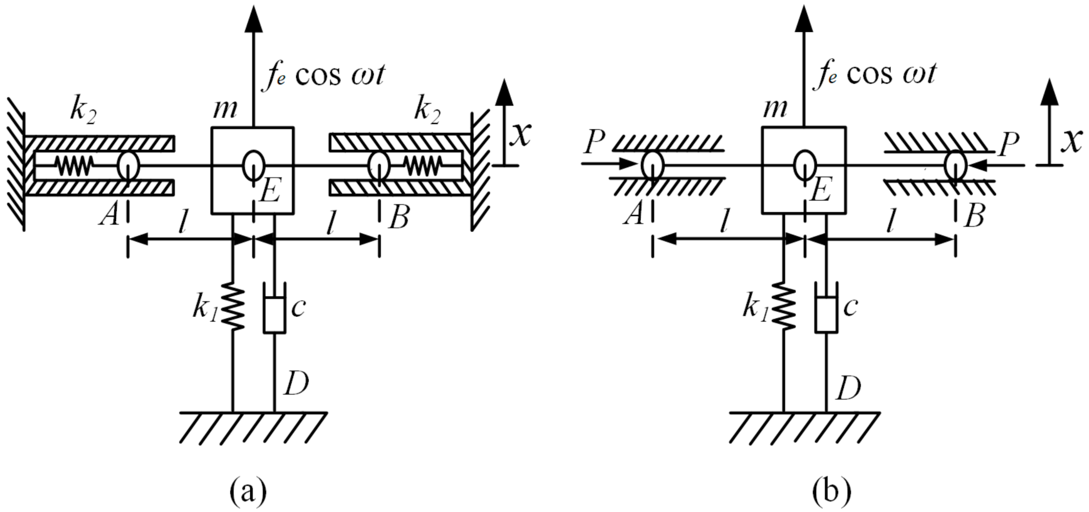
2.1. Model Description
2.2. Governing Equation
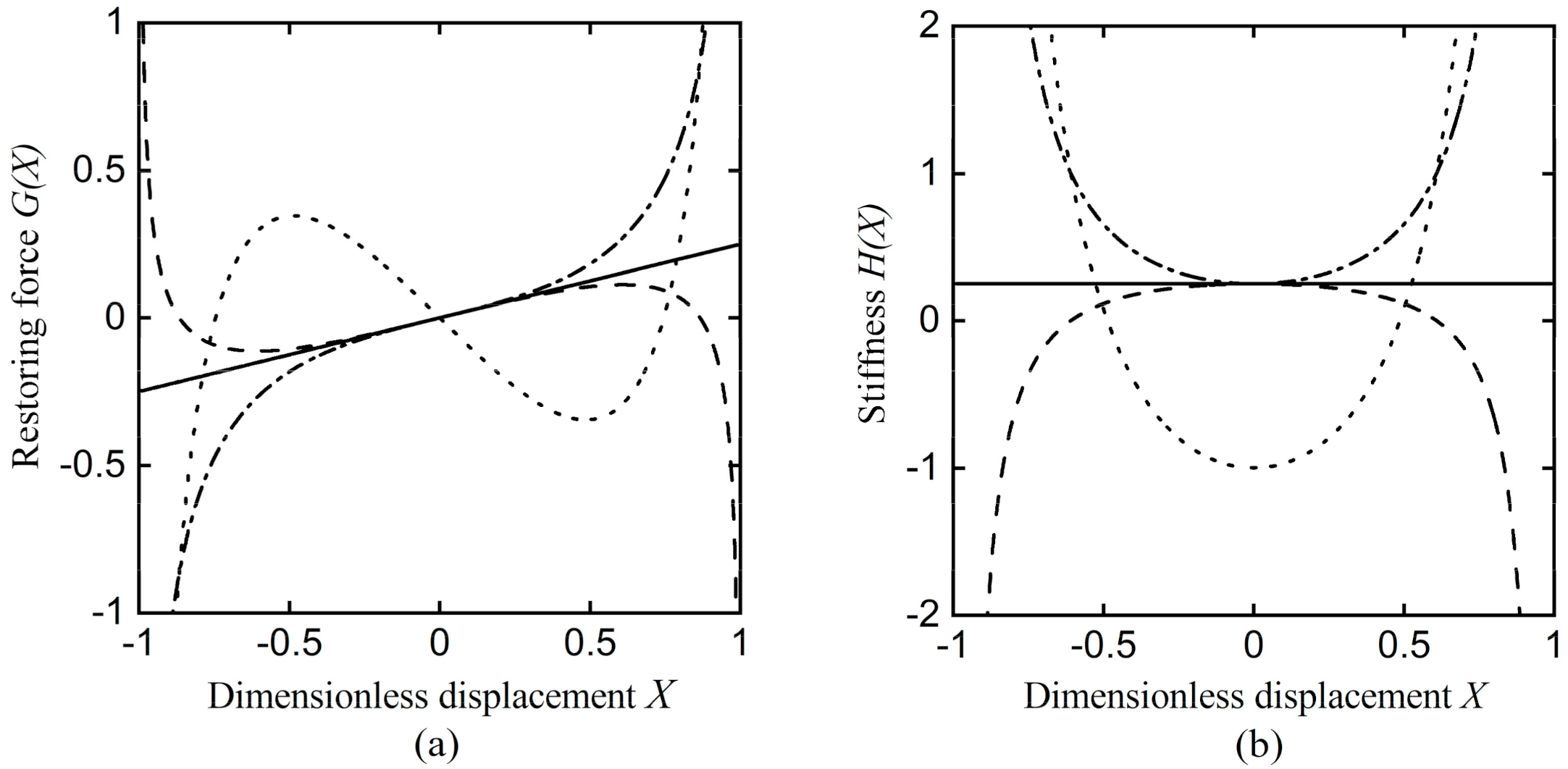
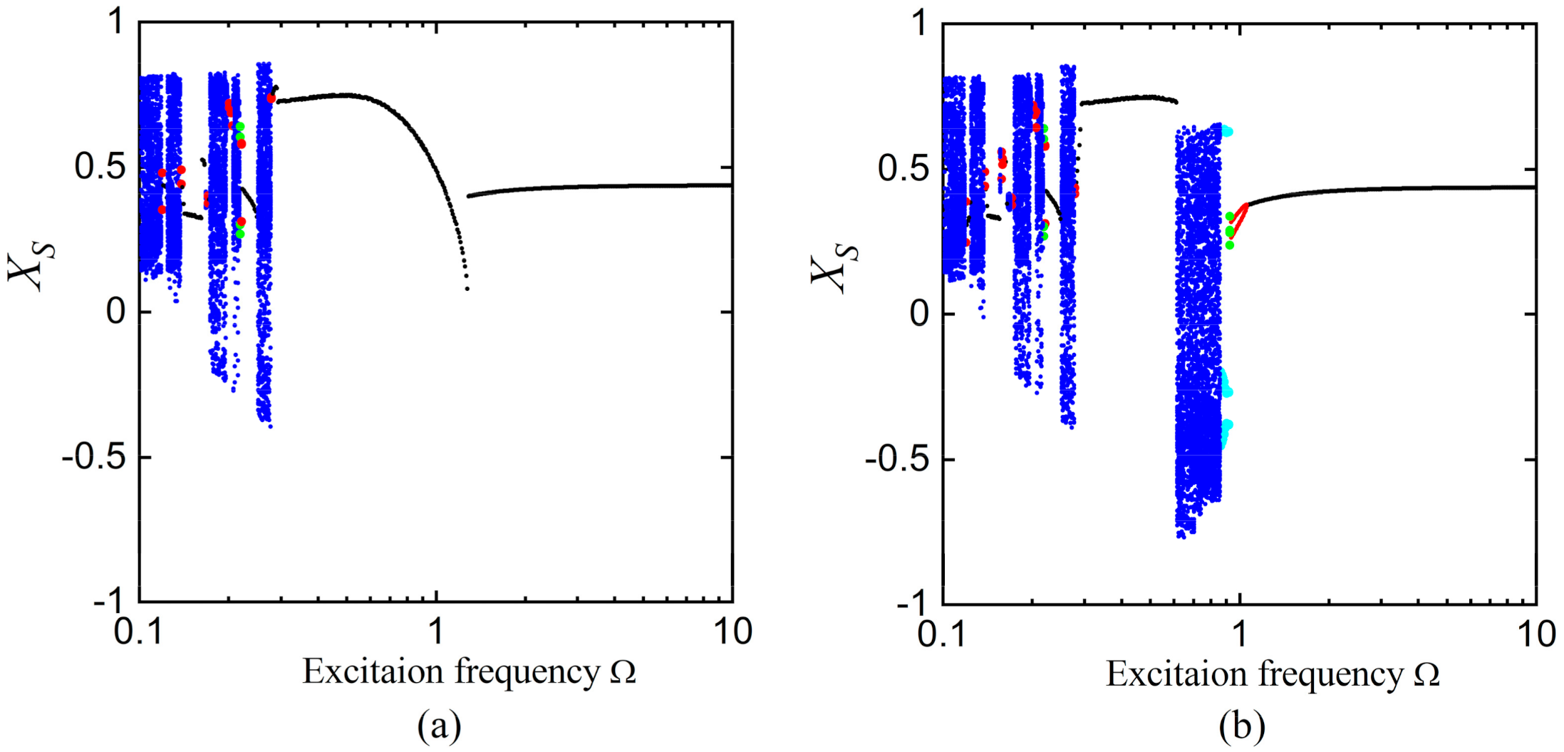
2.3. Stability Analysis
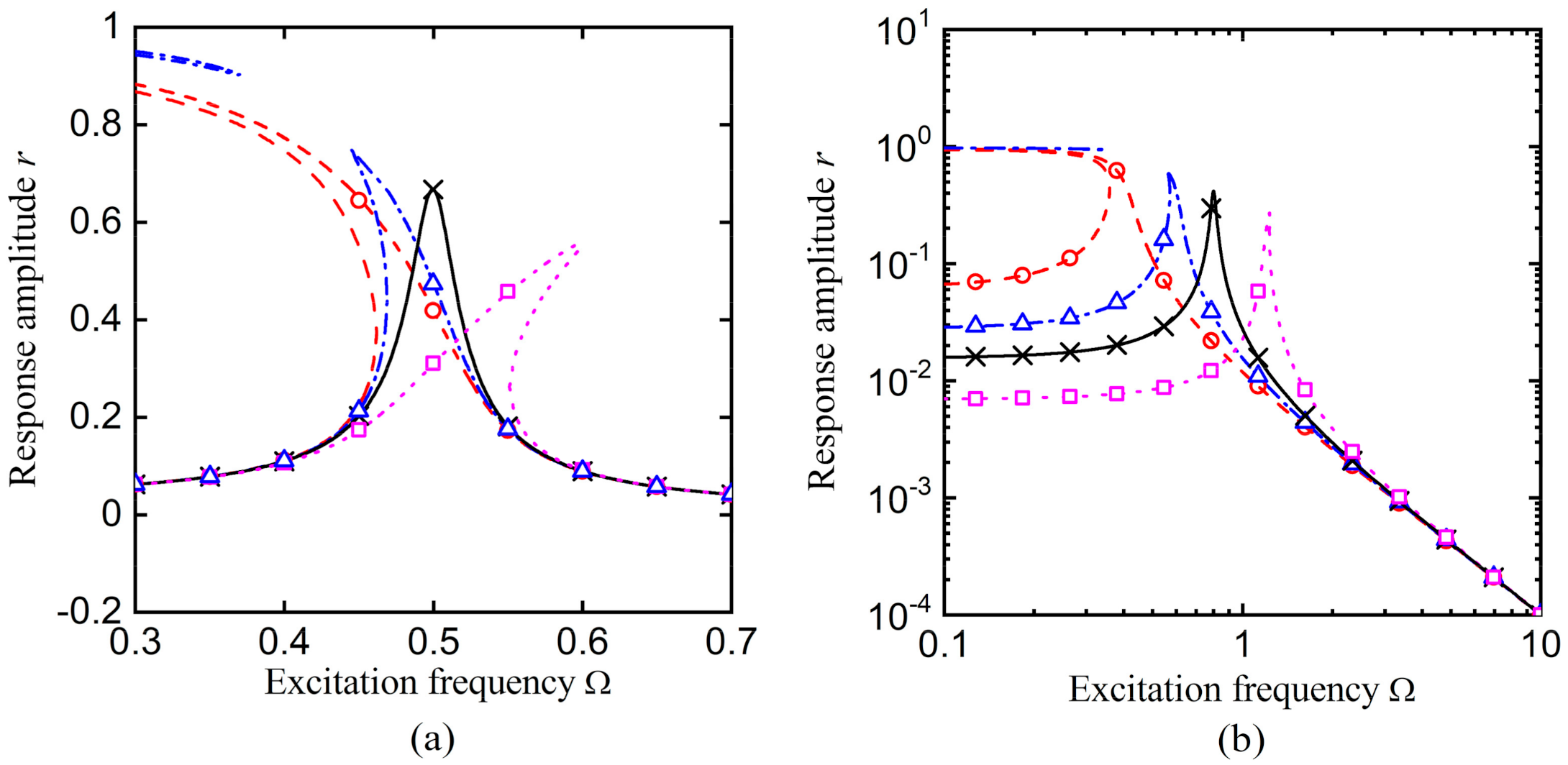
2.4. Frequency Response Function
3. Force Transmission and Power Flow Analysis
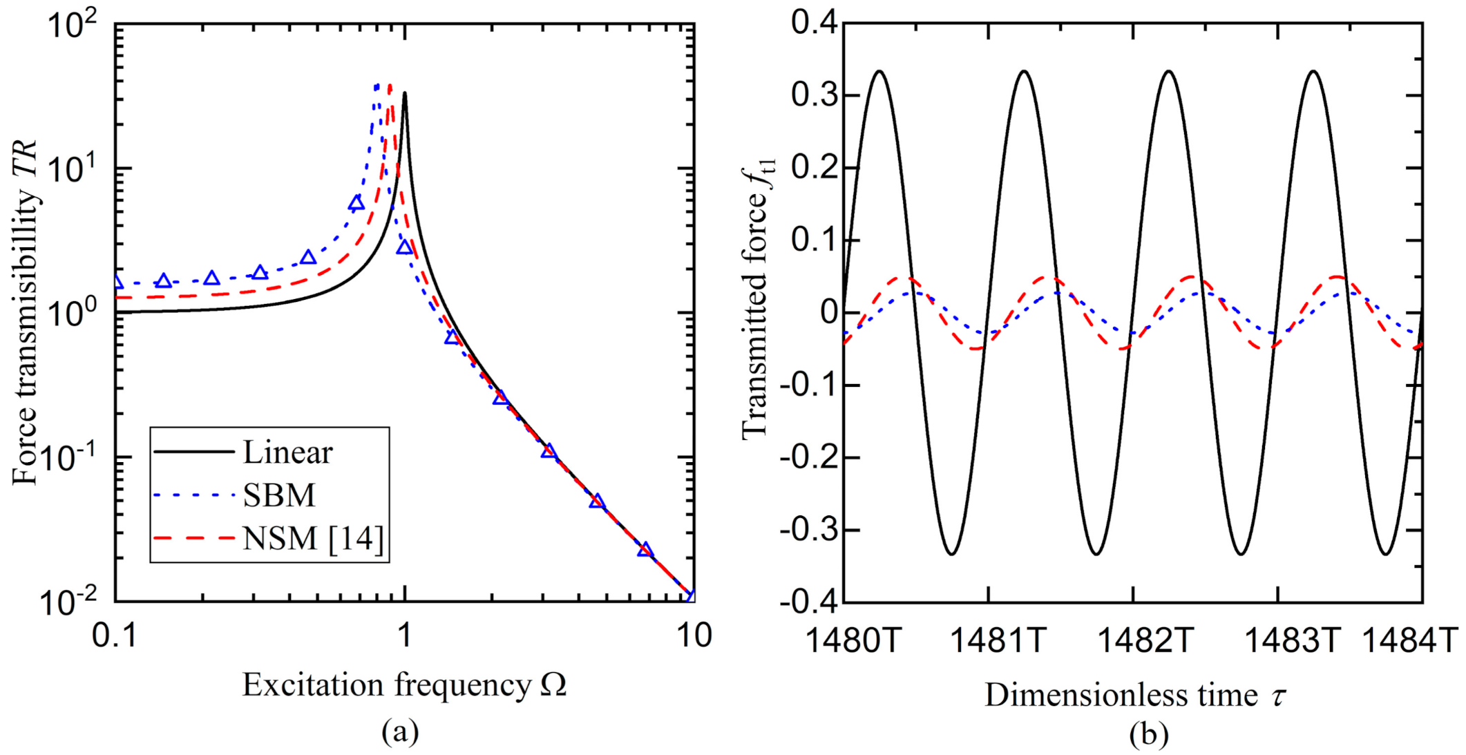
3.1. Force Transmisibillity
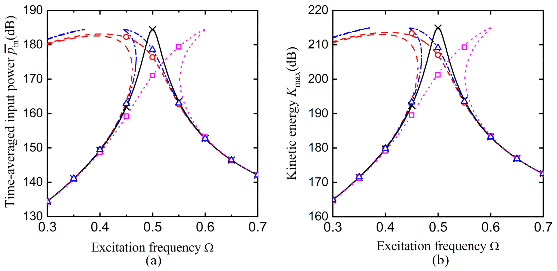
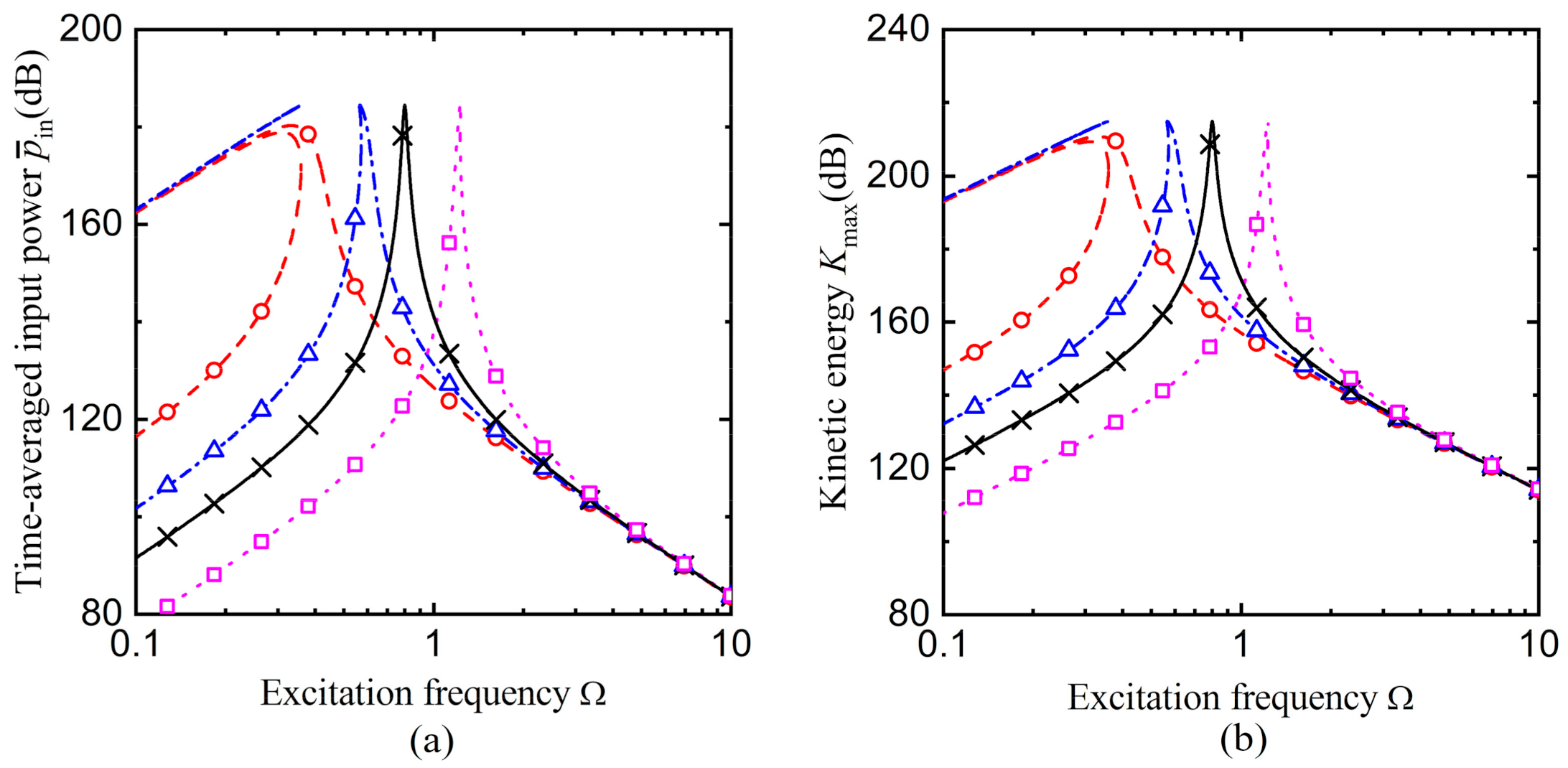
3.2. Time-Averaged Input Power and Kinetic Energy
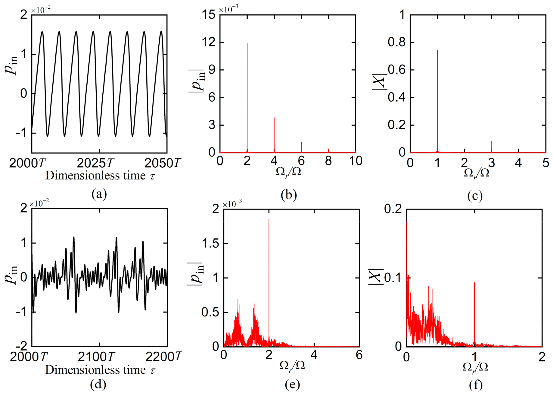
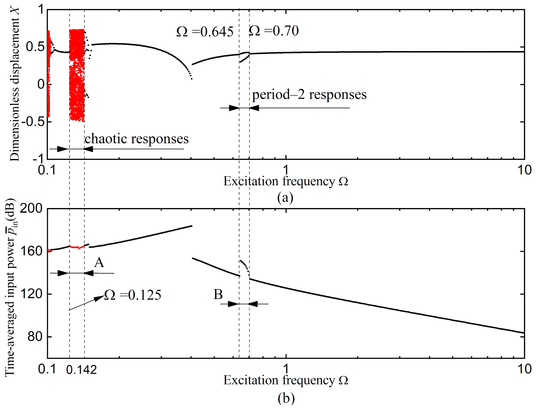
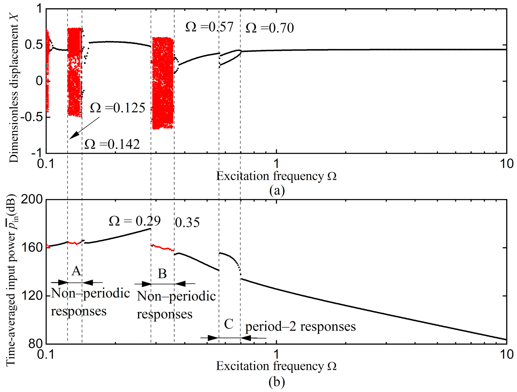
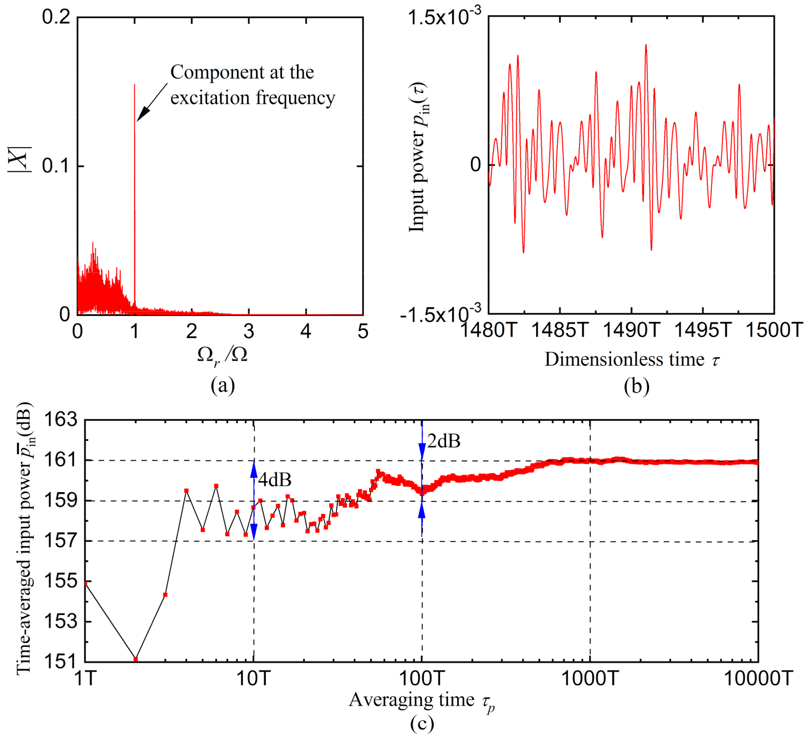
3.3. Non-Periodic Response
4. Conclusions
Author Contributions
Funding
Institutional Review Board Statement
Informed Consent Statement
Data Availability Statement
Acknowledgments
Conflicts of Interest
References
- Harris, C.M.; Crede, C.E. Shock and Vibration Handbook; McGraw-Hill: New York, NY, USA, 1961. [Google Scholar]
- Den Hartog, J.P. Mechanical Vibration; Dover Publications Inc.: New York, NY, USA, 1985. [Google Scholar]
- Yilmaz, C.; Kikuchi, N. Analysis and design of passive band-stop filter-type vibration isolators for low-frequency applications. J. Sound Vib. 2006, 291, 1004–1028. [Google Scholar] [CrossRef]
- Xing, J.T.; Xiong, Y.P.; Price, W.G. Passive-active vibration isolation systems to produce zero or infinite dynamic modulus: Theoretical and conceptual design strategies. J. Sound Vib. 2005, 286, 615–636. [Google Scholar] [CrossRef]
- Alabuzhev, P.; Gritchin, A.; Kim, L.; Migirenko, G.; Chon, V.; Stepanov, P. Vibration Protecting and Measuring Systems with Quasi-Zero Stiffness; Hemisphere: New York, NY, USA, 1989. [Google Scholar]
- Platus, D.L. Negative-stiffness-mechanism vibration isolation system. In Proceedings of the SPIE-The International Society for Optical Engineering, Vibration Control in Microelectronics, Optics, and Metrology, San Jose, CA, USA, 4–6 November; 1992; pp. 44–54. [Google Scholar]
- Carrella, A.; Brennan, M.J.; Waters, T.P. Static analysis of a passive vibration isolator with quasi-zero-stiffness characteristic. J. Sound Vib. 2007, 301, 678–689. [Google Scholar] [CrossRef]
- Lee, C.M.; Goverdovskiy, V.N.; Temnikov, A.I. Design of springs with “negative” stiffness to improve vehicle driver vibration isolation. J. Sound Vib. 2007, 302, 865–874. [Google Scholar] [CrossRef]
- Kovavic, I.; Brennan, M.J.; Waters, T.P. A study of a nonlinear vibration isolator with a quasi-zero stiffness characteristic. J. Sound Vib. 2008, 315, 700–711. [Google Scholar] [CrossRef]
- Lu, Z.Q.; Yang, T.; Brennan, M.J.; Liu, Z.; Chen, L.-Q. Experimental Investigation of a Two-stage Nonlinear Vibration Isolation System with High-static-Low-Dynamic Stiffness. J. Appl. Mech. 2017, 84, 021001. [Google Scholar] [CrossRef]
- Carrella, A.; Brennan, M.J.; Waters, T.P.; Shin, K. On the design of a high-static-low-dynamic stiffness isolator using linear mechanical springs and magnets. J. Sound Vib. 2008, 315, 712–720. [Google Scholar] [CrossRef]
- Lu, Z.Q.; Wu, D.; Ding, H.; Chen, L.-Q. Vibration isolation and energy harvesting integrated in a Stewart platform with high static and low dynamic stiffness. Appl. Math. Model. 2021, 89, 249–267. [Google Scholar] [CrossRef]
- Cao, Q.; Xiong, Y.P.; Wiercigroch, M. A novel model of dipteran flight mechanism. Int. J. Dynam. Control 2013, 1, 1–11. [Google Scholar] [CrossRef] [Green Version]
- Yang, J.; Xiong, Y.P.; Xing, J.T. Dynamics and power flow behaviour of a nonlinear vibration isolation system with a negative stiffness mechanism. J. Sound Vib. 2013, 332, 167–183. [Google Scholar] [CrossRef]
- Lu, Z.Q.; Gu, D.-H.; Ding, H.; Lacarbonara, W.; Chen, L.-Q. Nonlinear vibration isolation via a circular ring. Mech. Syst. Signal Process. 2020, 136, 106490. [Google Scholar] [CrossRef]
- Shaw, A.D.; Neild, S.A.; Wagg, D.J.; Weaver, P.M.; Carella, A. A nonlinear spring mechanism incorporating a bistable composite plate for vibration isolation. J. Sound Vib. 2013, 332, 65–75. [Google Scholar] [CrossRef] [Green Version]
- Yan, B.; Ma, H.; Zhang, L.; Zheng, W.; Wang, K.; Wu, C. A bistable vibration isolator with nonlinear electromagnetic shunt damping. Mech. Syst. Signal Process. 2020, 136, 106504. [Google Scholar] [CrossRef]
- Yan, B.; Ma, H.; Yu, N.; Zhang, L.; Wu, C. Theoretical modeling and experimental analysis of nonlinear electromagnetic shunt damping. J. Sound Vib. 2020, 471, 115184. [Google Scholar] [CrossRef]
- Zhang, L.; Zhao, C.; Qian, F.; Dhupia, J.S.; Wu, M. A Variable Parameter Ambient Vibration Control Method Based on Quasi-Zero Stiffness in Robotic Drilling Systems. Machines 2021, 9, 67. [Google Scholar] [CrossRef]
- Meng, Q.; Yang, X.; Li, W.; Lu, E.; Sheng, L. Research and Analysis of Quasi-Zero-Stiffness Isolator with Geometric Nonlinear Damping. Shock Vib. 2017, 2017, 1–9. [Google Scholar] [CrossRef] [Green Version]
- Tuo, J.; Deng, Z.; Huang, W.; Zhang, H. A six degree of freedom passive vibration isolator with quasi-zero-stiffness-based supporting. J. Low Freq. Noise Vib. Act. Control 2018, 37, 279–294. [Google Scholar] [CrossRef] [Green Version]
- Le, T.D.; Ahn, K.K. A vibration isolation system in low frequency excitation region using negative stiffness structure for vehicle seat. J. Sound Vib. 2011, 330, 6311–6335. [Google Scholar] [CrossRef]
- Goyder, H.G.D.; White, R.G. Vibration power flow from machines into built-up structures. J. Sound Vib. 1980, 68, 59–117. [Google Scholar] [CrossRef]
- Pinnington, R.J.; White, R.G. Power flow through machine isolators to resonant and non-resonant beam. J. Sound Vib. 1981, 75, 179–197. [Google Scholar] [CrossRef]
- Royston, T.J.; Singh, R. Optimization of passive and active non-linear vibration mounting systems based on vibratory power transmission. J. Sound Vib. 1996, 194, 295–316. [Google Scholar] [CrossRef]
- Royston, T.J.; Singh, R. Vibratory power flow through a nonlinear path into a resonant receiver. J. Acoust. Soc. Am. 1997, 101, 2059–2069. [Google Scholar] [CrossRef]
- Zhu, C.; Yang, J.; Rudd, C. Vibration transmission and power flow of laminated composite plates with inerter-based suppression configurations. Int. J. Mech. Sci. 2021, 190, 106012. [Google Scholar] [CrossRef]
- Xiong, Y.P.; Xing, J.T.; Price, W.G. Interactive power flow characteristics of an integrated equipment--nonlinear isolator--travelling flexible ship excited by sea waves. J. Sound Vib. 2005, 287, 245–276. [Google Scholar] [CrossRef]
- Yang, J.; Xiong, Y.P.; Xing, J.T. Nonlinear power flow analysis of the Duffing oscillator. Mech. Syst. Signal Process. 2014, 45, 563–578. [Google Scholar] [CrossRef]
- Yang, J.; Xiong, Y.P.; Xing, J.T. Power flow behaviour and dynamic performance of a nonlinear vibration absorber coupled to a nonlinear oscillator. Nonlinear Dyn. 2015, 80, 1063–1079. [Google Scholar] [CrossRef]
- Yang, J.; Xiong, Y.P.; Xing, J.T. Vibration power flow and force transmission behaviour of a nonlinear isolator mounted on a nonlinear base. Int. J. Mech. Sci. 2016, 115–116, 238–252. [Google Scholar] [CrossRef]
- Yang, J.; Shi, B.; Rudd, C. On vibration transmission between Interactive oscillators with nonlinear coupling interface. Int. J. Mech. Sci. 2018, 137, 238–251. [Google Scholar] [CrossRef]
- Shi, B.; Yang, J.; Rudd, C. On vibration transmission in oscillating systems incorporating bilinear stiffness and damping elements. Int. J. Mech. Sci. 2019, 150, 458–470. [Google Scholar] [CrossRef]
- Shi, B.; Yang, J. Quantification of vibration transmission between coupled nonlinear oscillators. Int. J. Dynam. Control 2020, 8, 418–435. [Google Scholar] [CrossRef]
- Dai, W.; Yang, J.; Shi, B. Vibration transmission and power flow in impact oscillators with linear and nonlinear constraints. Int. J. Mech. Sci. 2020, 168, 105234. [Google Scholar] [CrossRef]
- Dai, W.; Yang, J. Vibration transmission and energy flow of impact oscillators with nonlinear motion constraints created by diamond-shaped linkage mechanism. Int. J. Mech. Sci. 2021, 194, 106212. [Google Scholar] [CrossRef]
- Yang, J.; Jiang, J.Z.; Neild, S. Dynamic analysis and performance evaluation of nonlinear inerter-based vibration isolators. Nonlinear Dyn. 2020, 99, 1823–1839. [Google Scholar] [CrossRef] [Green Version]
- Nayfeh, A.H.; Mook, D.T. Nonlinear Oscillations; Willey: New York, NY, USA, 1979. [Google Scholar]
- Abramowitz, M.; Stegun, I.A. Handbook of Mathematical Functions with Formulas, Graphs, and Mathematical Tables; Dover Publications: New York, NY, USA, 1972. [Google Scholar]
- Press, W.H.; Flannery, B.P.; Teukolsky, S.A.; Vetterling, W.T. Numerical Recipes: The Art of Scientific Computing; Cambridge University Press: Cambridge, UK, 1992. [Google Scholar]
- Wolf, A.; Swift, J.B.; Swinney, H.L.; Vastano, J.A. Determining Lyapunov exponents from a time series. Phys. D 1985, 16, 285–317. [Google Scholar] [CrossRef] [Green Version]
- Nayfeh, A.H.; Balachandran, B. Applied Nonlinear Dynamics: Analytical, Computational, and Experimental Methods; Wiley: New York, NY, USA, 1995. [Google Scholar]


| Parameter Values | System Characteristics | |
|---|---|---|
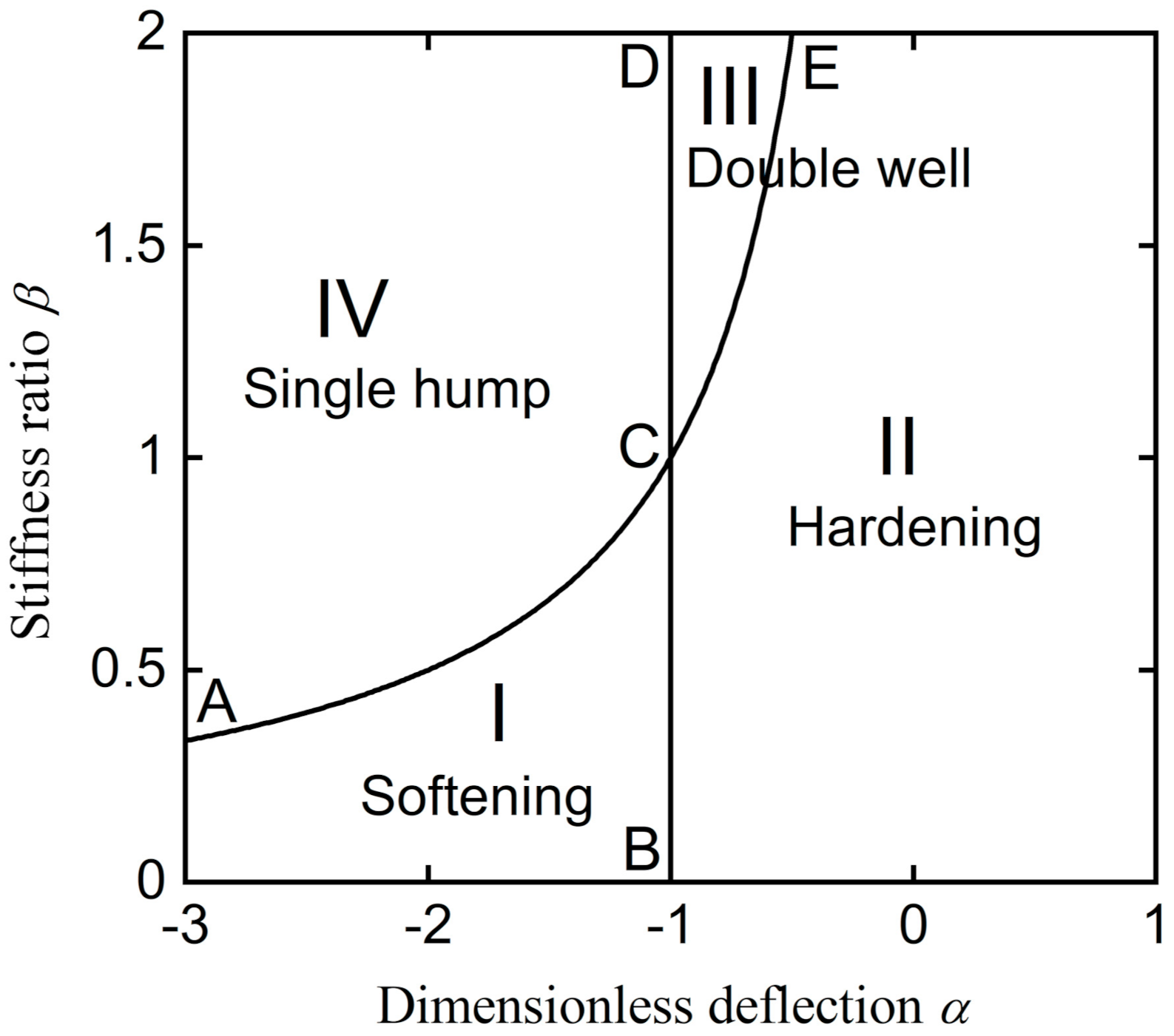
| Line ACE | ||
| Line BCD | Linear system | |
| Region I | , | Softening stiffness system |
| Region II | , | Hardening stiffness system |
| Region III | , | Double-well potential system |
| Region IV | , | Single-hump potential system |
Publisher’s Note: MDPI stays neutral with regard to jurisdictional claims in published maps and institutional affiliations. |
© 2021 by the authors. Licensee MDPI, Basel, Switzerland. This article is an open access article distributed under the terms and conditions of the Creative Commons Attribution (CC BY) license (https://creativecommons.org/licenses/by/4.0/).
Share and Cite
Shi, B.; Yang, J.; Li, T. Enhancing Vibration Isolation Performance by Exploiting Novel Spring-Bar Mechanism. Appl. Sci. 2021, 11, 8852. https://doi.org/10.3390/app11198852
Shi B, Yang J, Li T. Enhancing Vibration Isolation Performance by Exploiting Novel Spring-Bar Mechanism. Applied Sciences. 2021; 11(19):8852. https://doi.org/10.3390/app11198852
Chicago/Turabian StyleShi, Baiyang, Jian Yang, and Tianyun Li. 2021. "Enhancing Vibration Isolation Performance by Exploiting Novel Spring-Bar Mechanism" Applied Sciences 11, no. 19: 8852. https://doi.org/10.3390/app11198852
APA StyleShi, B., Yang, J., & Li, T. (2021). Enhancing Vibration Isolation Performance by Exploiting Novel Spring-Bar Mechanism. Applied Sciences, 11(19), 8852. https://doi.org/10.3390/app11198852