Soft Computing Paradigms to Find the Numerical Solutions of a Nonlinear Influenza Disease Model

Sabir, Zulqurnain; Ag Ibrahim, Ag Asri; Raja, Muhammad Asif Zahoor; Nisar, Kashif; Umar, Muhammad; Rodrigues, Joel J. P. C.; Mahmoud, Samy R.

doi:10.3390/app11188549

Open AccessArticle

Soft Computing Paradigms to Find the Numerical Solutions of a Nonlinear Influenza Disease Model

¹

Department of Mathematics and Statistics, Hazara University, Mansehra 21300, Pakistan

²

Faculty of Computing and Informatics, Universiti Malaysia Sabah, Jalan UMS, Kota Kinabalu 88400, Sabah, Malaysia

³

Future Technology Research Center, National Yunlin University of Science and Technology, 123 University Road, Section 3, Douliou 64002, Yunlin, Taiwan

⁴

Post-Graduation Program in Electrical Engineering, Federal University of Piauí (UFPI), Teresina 64049-550, Brazil

⁵

Covilhã Delegation, Instituto de Telecomunicações, 6201-001 Covilhã, Portugal

⁶

GRC Department, Faculty of Applied Studies, King Abdulaziz University, Jeddah 21589, Saudi Arabia

^*

Author to whom correspondence should be addressed.

Appl. Sci. 2021, 11(18), 8549; https://doi.org/10.3390/app11188549

Submission received: 13 May 2021 / Revised: 13 June 2021 / Accepted: 14 June 2021 / Published: 14 September 2021

(This article belongs to the Special Issue Application of Evolutionary Computation)

Download

Browse Figures

Versions Notes

Abstract

:

The aim of this work is to present the numerical results of the influenza disease nonlinear system using the feed forward artificial neural networks (ANNs) along with the optimization of the combination of global and local search schemes. The genetic algorithm (GA) and active-set method (ASM), i.e., GA-ASM, are implemented as global and local search schemes. The mathematical nonlinear influenza disease system is dependent of four classes, susceptible S(u), infected I(u), recovered R(u) and cross-immune individuals C(u). For the solutions of these classes based on influenza disease system, the design of an objective function is presented using these differential system equations and its corresponding initial conditions. The optimization of this objective function is using the hybrid computing combination of GA-ASM for solving all classes of the influenza disease nonlinear system. The obtained numerical results will be compared by the Adams numerical results to check the authenticity of the designed ANN-GA-ASM. In addition, the designed approach through statistical based operators shows the consistency and stability for solving the influenza disease nonlinear system.

Keywords:

influenza disease system; Adams methods; artificial neural networks; active-set method; genetic algorithms; statistical performances

1. Introduction

There are various serious diseases produced by viruses, of which influenza is one of them that primarily attacks the upper respiratory portions, bronchi, nose, throat and sometimes disturbs the lungs. The influenza is not a fatal illness, and most people recover within one to two weeks without medical care. This disease is a serious risk to older people or those with serious illnesses such as cancer, diabetes, heart, kidney problems and lung disease. Among these people, infection can lead to serious problems of primary diseases, such as pneumonia causing death. The epidemic rate of influenza is reported as between 5% and 15% per year of the population, which is affected by upper respiratory tract infections. Worldwide, the annual epidemics are witnessed between 3 and 5 million cases of serious illness and the number of deaths is reported to be around 250,000 and 500,000 [1]. Many mathematical epidemiological models are illustrated by the ordinary nonlinear autonomous differential systems, which designate the assumptions of the model that the parameters are time independent. In such systems, variables refer to recovered, infected, transmitted and susceptible disease vectors.

Astuti et al. [2] suggested a step-by-step differential transformation approach to solving the disease-resistant influenza virus model. Erdem et al. [3] presented mathematical investigations of a susceptible–infectious–quarantine–recovered (SIQR) influenza model with imperfect quarantine. Alzahrani and Khan [4] introduced a numerical technique to solve a fractional pandemic influenza model. Sun et al. [5] presented multi-objective optimization models for allocating patients during a pandemic influenza outbreak. Ghanbari et al. [6] provided an analysis of two models of avian influenza outbreaks relating fractal-fractional derivatives with power and memorabilia from Mittag-Leffler. González-Parra et al. [7] designed and discussed a fractional epidemiological model for simulating influenza A outbreak. Tchuenche et al. [8] researched the impact of media coverage on human influenza transmission dynamics. Schulze-Horsel et al. [9] discussed the dynamics of infection and virus-induced apoptosis in the production of influenza vaccines in cellular culture. Hovav et al. [10] presented a network flow system for managing inventory and distributing influenza vaccines in a healthcare supply chain. Patel et al. [11] used genetic algorithms to discuss the optimal vaccination plans for pandemic influenza. Kanyiri et al. [12] introduced the optimum control applications for influenza and pulmonary congestion with antiviral resistance.

The influenza disease nonlinear system has four categories, susceptible (S(u)), infectious (I(u)), recovered (R(u)) and cross-immune (C(u)). The mathematical design of the nonlinear influenza disease system is written as follows [13]:

{\begin{cases} S^{'} (u) = μ - (β I (u) + μ) S (u) + γ C (u), & S (0) = a_{1}, \\ I^{'} (u) = β (S (t) + σ C (u)) I (u) - (α + μ) I (u), & I (0) = a_{2}, \\ R^{'} (u) = α I (u) + β (1 - σ) C (u) I (u) - (μ + δ) R (u), & R (0) = a_{3}, \\ C^{'} (u) = δ R (u) - (γ + β I (u) + μ) C (u), & C (0) = a_{4}, \end{cases},

(1)

where β shows the transmission rate for the susceptible to the infected individual, and a₁, a₂, a₃ and a₄ are the initial conditions. The infected, infectious and cross-immune are signified as γ⁻¹, δ⁻¹ and α⁻¹, respectively. σ shows the exposed cross-immune individuals, who are shifted in a unit time to transmittable subpopulations [14]. The recently reported studies addressing the different aspect of influenza nonlinear modelling can be seen in [15,16,17,18,19].

The aim of this work is to solve the above nonlinear influenza disease model using the stochastic capabilities of artificial neural networks (ANNs), genetic algorithms (GA) and the active set method (ASM), i.e., ANN-GA-ASM. Stochastic numerical methods have been implemented to solve a great number of applications, such as singular fractional models, COVID-19-based susceptible–infectious–treatment–recovered (SITR) dynamics, the delay singular functional model, the prey–predator model, singular higher order nonlinear models, the dengue fever nonlinear system, multi-singular differential models and the mosquito release nonlinear system based on the heterogeneous environment (please see [20,21] and citation therein). Based on these well-known applications, the authors are interested in solving the nonlinear influenza system using the ANN-GA-ASM. Few key factors of the ANN-GA-ASM are briefly given as:

The proposed ANN-GA-ASM provides effective solutions of the nonlinear influenza system.
Consistent, stable and reliable outcomes from the nonlinear influenza system validate the value of the proposed ANN-GA-ASM.
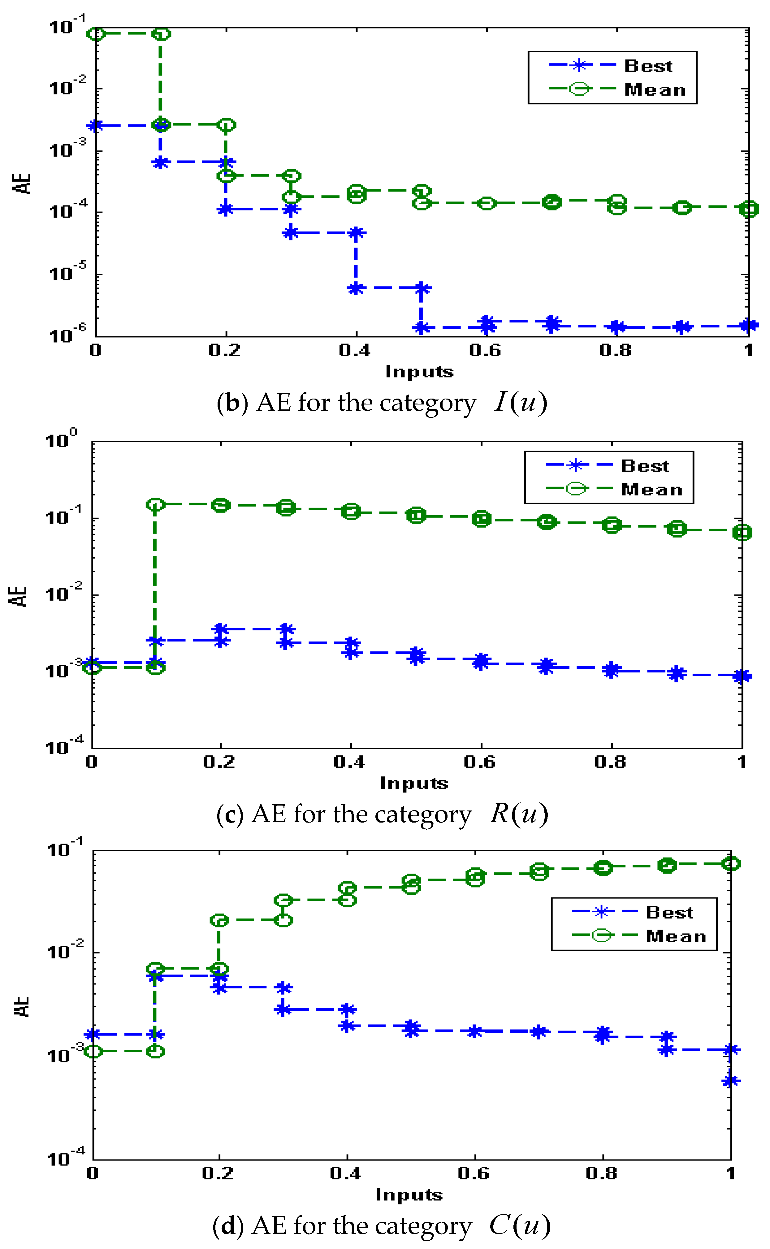
The absolute error (AE) values are in the good agreements, indicating the reliability of the proposed ANN-GA-ASM.
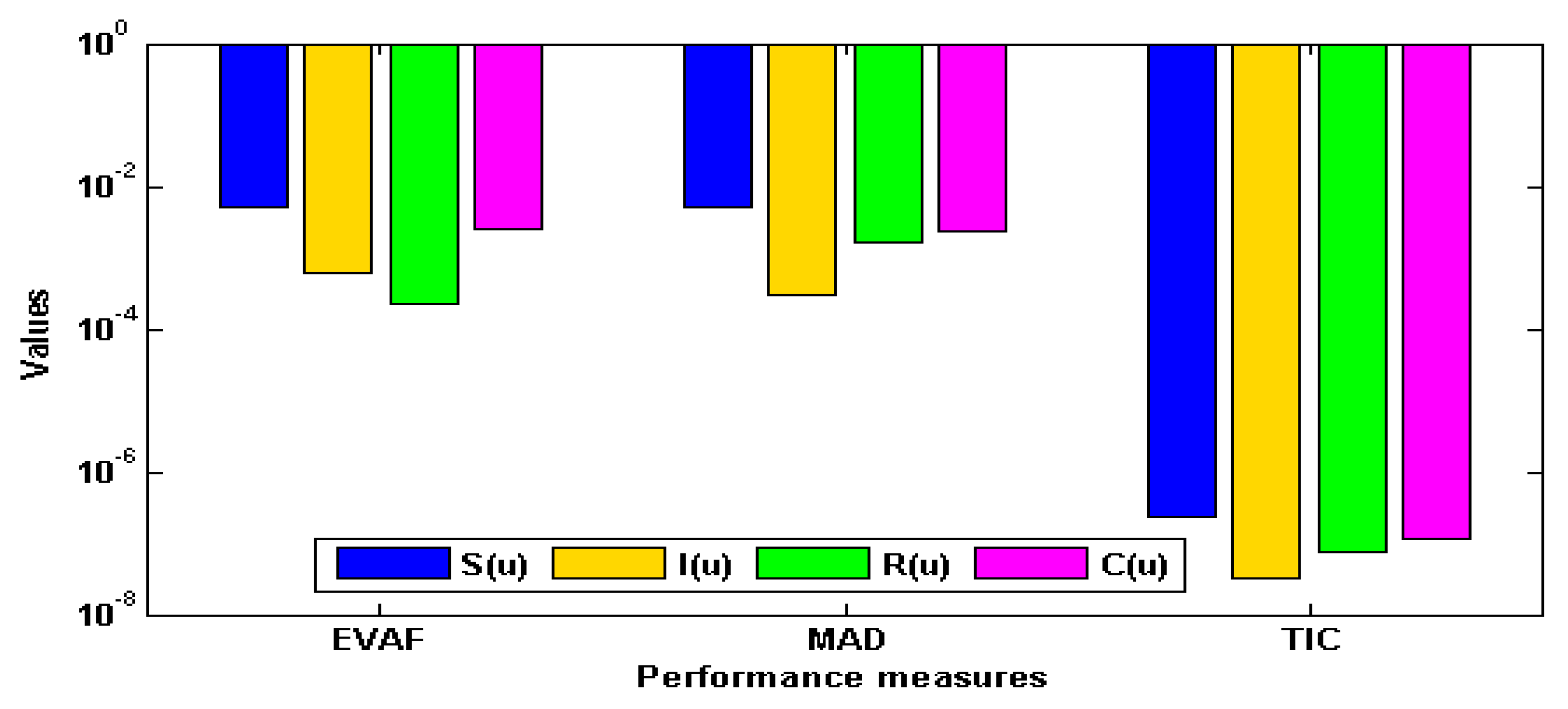
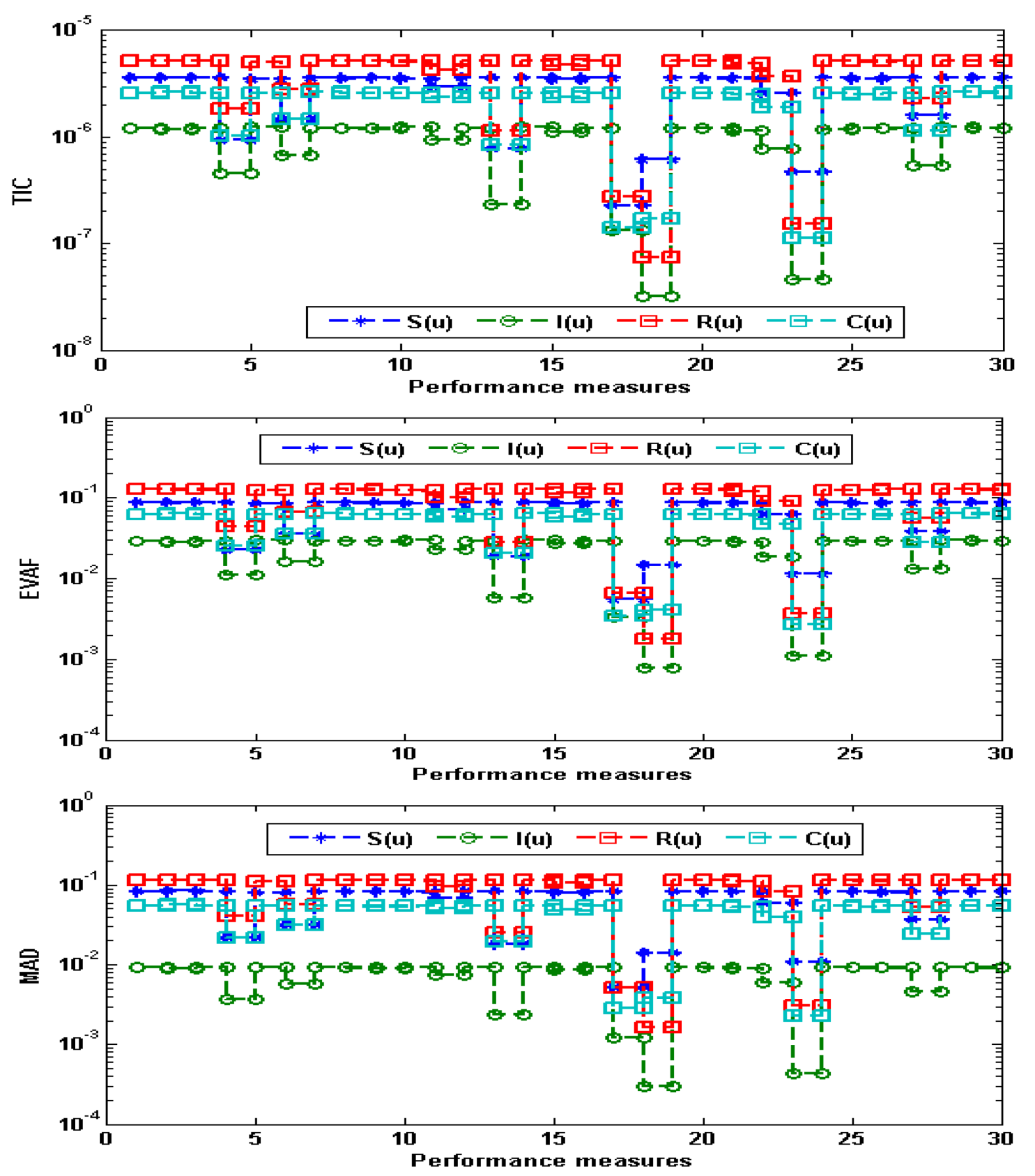
The performance is certified through ANN-GA-ASM using different statistical observations to solve the nonlinear influenza system for thirty independent trials.
The designed ANN-GA-ASM is effortlessly implemented to solve the nonlinear influenza system with smooth operations, inclusive and easy to understand.

The other paper parts are as follows. Section 2 shows the methodology and statistical measures. Section 3 demonstrates the simulation of the outcomes. Section 4 provides the final remarks and future research remarks.

2. Methodology

The methodology of the proposed ANN-GA-ASM structure to solve the nonlinear influenza system is defined in two steps: an objective function is designed to solve the ANN parameters and some crucial settings are provided to improve the objective function based on the GA-ASM.

2.1. ANN Structure

In this section, the mathematical design is presented to solve each category of the susceptible (S), infectious (I), recovered (R) and cross-immune (C) groups based on the influenza disease system. The proposed outcomes of these classes are

\hat{S}, \hat{I}, \hat{R}

and

\hat{C}

given as:

[\hat{S} (u), \hat{I} (u), \hat{R} (u), \hat{C} (u)] = [\begin{array}{l} \sum_{k = 1}^{m} p_{S, k} v (w_{S, k} u + q_{S, k}), \sum_{k = 1}^{m} p_{I, k} v (w_{I, k} u + q_{I, k}), \\ \sum_{k = 1}^{m} p_{R, k} v (w_{R, k} u + q_{R, k}), \sum_{k = 1}^{m} p_{C, k} v (w_{C, k} u + q_{C, k}) \end{array}], [{\hat{S}}^{'} (u), {\hat{I}}^{'} (u), {\hat{R}}^{'} (u), {\hat{C}}^{'} (u)] = [\begin{array}{l} \sum_{k = 1}^{m} p_{S, k} v^{'} (w_{S, k} u + q_{S, k}), \sum_{k = 1}^{m} p_{I, k} v^{'} (w_{I, k} u + q_{I, k}), \\ \sum_{k = 1}^{m} p_{R, k} v^{'} (w_{R, k} u + q_{R, k}), \sum_{k = 1}^{m} p_{C, k} v^{'} (w_{C, k} u + q_{C, k}) \end{array}],

(2)

where m is number of neurons, and W is the unknown weight vector, with its components for S, I, R and C are defined as W_S, W_I, W_R and W_C, respectively, and are given mathematically as follows:

\begin{matrix} W = [W_{S}, W_{I}, W_{R}, W_{C}], for W_{S} = [p_{S}, w_{S}, q_{S}], W_{I} = [p_{I}, w_{I}, q_{I}], W_{R} = [p_{R}, w_{R}, q_{R}] and \\ W_{C} = [p_{C}, w_{C}, q_{C}], for \\ p_{S} = [p_{S, 1}, p_{S, 2}, \dots, p_{S, m}], p_{I} = [p_{I, 1}, p_{I, 2}, \dots, p_{I, m}], p_{R} = [p_{R, 1}, p_{R, 2}, \dots, p_{R, m}], \\ p_{C} = [p_{C, 1}, p_{C, 2}, \dots, p_{C, m}], w_{S} = [w_{S, 1}, w_{S, 2}, \dots, w_{S, m}], w_{I} = [w_{I, 1}, w_{I, 2}, \dots, w_{I, m}], \\ w_{R} = [w_{R, 1}, w_{R, 2}, \dots, w_{R, m}], w_{C} = [w_{C, 1}, w_{C, 2}, \dots, w_{C, m}], q_{S} = [q_{S, 1}, q_{S, 2}, \dots, q_{S, m}], \\ q_{I} = [q_{I, 1}, q_{I, 2}, \dots, q_{I, m}], q_{R} = [q_{R, 1}, q_{R, 2}, \dots, q_{R, m}], q_{C} = [q_{C, 1}, q_{C, 2}, \dots, q_{C, m}] . \end{matrix}

(3)

The updated form by applying the log-sigmoid function

v (μ) = {(1 + \exp (- μ))}^{- 1}

is provided in Appendix A for the interested readers. To find the optimization measures, an error based objective function becomes:

E = E_{1} + E_{2} + E_{3} + E_{4} + E_{5},

(4)

E_{1} = \frac{1}{N} \sum_{k = 1}^{N} {[{\hat{S}}_{k}^{'} - μ + (β {\hat{I}}_{k} + μ) {\hat{S}}_{k} - γ {\hat{C}}_{k}]}^{2},

(5)

E_{2} = \frac{1}{N} \sum_{k = 1}^{N} {[{\hat{I}}_{k}^{'} - β {\hat{S}}_{k} {\hat{I}}_{k} + μ {\hat{I}}_{k} + σ {\hat{I}}_{k} - σ C_{k} {\hat{I}}_{k}]}^{2},

(6)

E_{3} = \frac{1}{N} \sum_{k = 1}^{N} {[{\hat{R}}_{k}^{'} - α {\hat{I}}_{k} - β (1 - σ) {\hat{C}}_{k} {\hat{I}}_{k} + (μ + δ) {\hat{R}}_{k}]}^{2},

(7)

E_{4} = \frac{1}{N} \sum_{k = 1}^{N} {[{\hat{C}}_{k}^{'} - δ {\hat{R}}_{k} + (γ + β {\hat{I}}_{k} + μ) {\hat{C}}_{k}]}^{2},

(8)

E_{5} = \frac{1}{4} [{({\hat{S}}_{0} - a_{1})}^{2} + {({\hat{I}}_{0} - a_{2})}^{2} + {({\hat{R}}_{0} - a_{3})}^{2} + + {({\hat{C}}_{0} - a_{4})}^{2}],

(9)

where

{\hat{S}}_{k} = S (u_{k}), {\hat{I}}_{k} = I (u_{k}), {\hat{R}}_{k} = R (u_{k})

and

{\hat{C}}_{k} = C (μ_{k})

. In the above network

E_{1},

E_{2},

E_{3}

and

E_{4}

indicate the objective functions related to system (1), while

E_{5}

is designed on the basis of the initial conditions of system (1).

2.2. Optimization Performances: GA-ASM

In this section, the ANN-GA-ASM performance is presented for solving the influenza disease nonlinear system. The designed ANN structure through GA-ASM for solving the influenza disease nonlinear system is depicted in Figure 1. The block structure of the proposed methodologies is illustrated by defining the problem, mathematical modeling, the formulation of the fitness function on mean square error sense, the workflow of GA and ASM.

In this study, the global search GA is one of optimization process that is executed to solve the influenza disease nonlinear system. GA is pragmatic to standardize the specific population for solving the various complicated models using the optimal training. To achieve the best system outcomes, GA operates through a selection operator, a crossover process, reproduction practice and a mutation procedure. Recently, GA has been applied in the hospitalization expenditure system [22], for feature assortment in cancer microarray [23], brain tumor images [24], air blast prediction [25], monorail vehicle dynamics [26], cloud service optimization [27] and liver disease prediction [28].

The active-set method is one of the rapid local search optimization approaches that works to solve the constrained/unconstrained models broadly. ASM is executed in numerous optimizations models of numerous complex and non-stiff systems. Recently, ASM is applied to execute the real-time optimal control [29], the pricing of American better-of option on two assets [30], the pressure-dependent model of water distribution systems [31], overcurrent relays in microgrid optimization [32], embedded model predictive controls [33] and elastodynamic frictional contact problems [34]. To control the slowness of GA, the process of hybridization into GA-ASM is provided in Table 1 for training or learning of the decision variables, i.e., the unknown weights of ANNs, while the parameter settings of GA and ASM are handled using the ‘optimset’ routine of the Matlab optimization toolbox. The setting of the parameters, i.e., fitness function tolerance (TolFun), constraints tolerance (TolCon), population size (PopSiz), generations, Stall generation limits (StallLimit), decision variable tolerance (TolX), iteration and maximum number of fitness function evalutions (MaxFunEvals), is done with care to avoid the premature convergence of the optimization mechanism.

2.3. Performance Measures

The mathematical representations using the statistical operators containing “variance account for (VAF)”, “mean absolute deviation (MAD)”, “semi-interquartile (S.I.R)” and

“Theil’s inequality coefficient (TIC)” along with their Global representations are presented to solve the influenza disease nonlinear model and are provided in Appendix B.

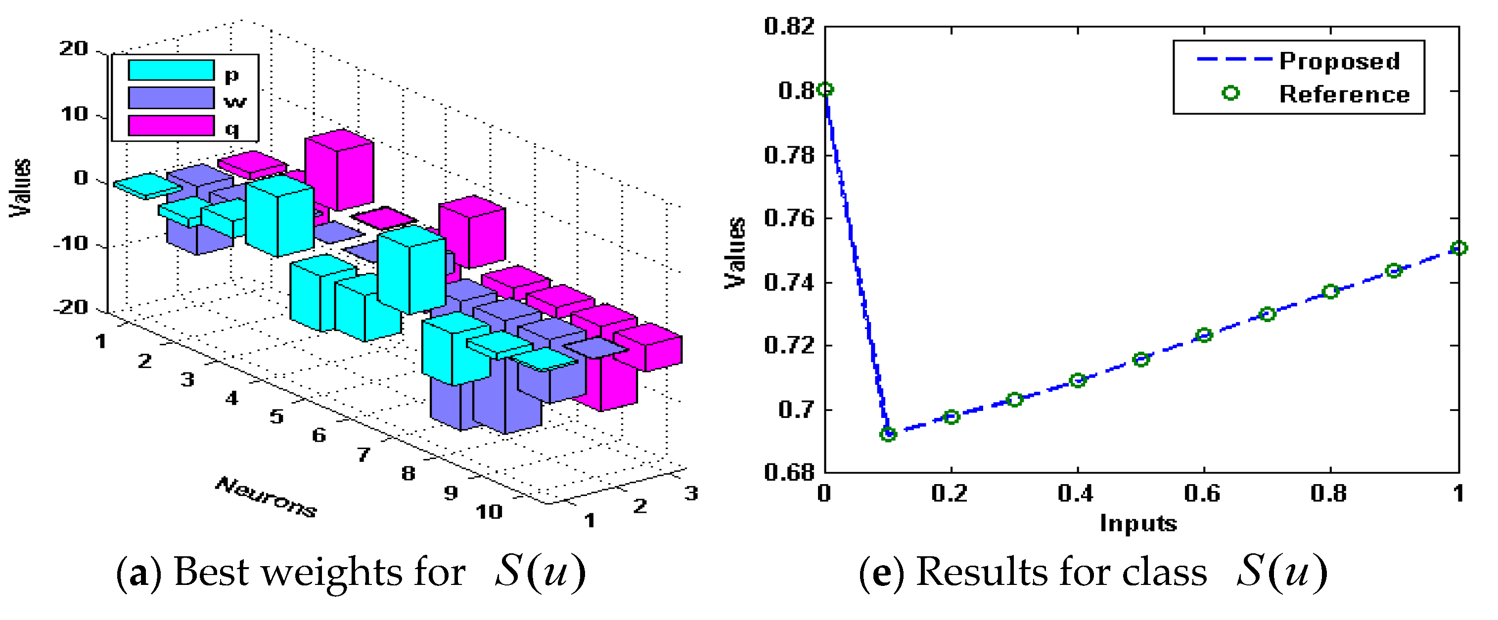
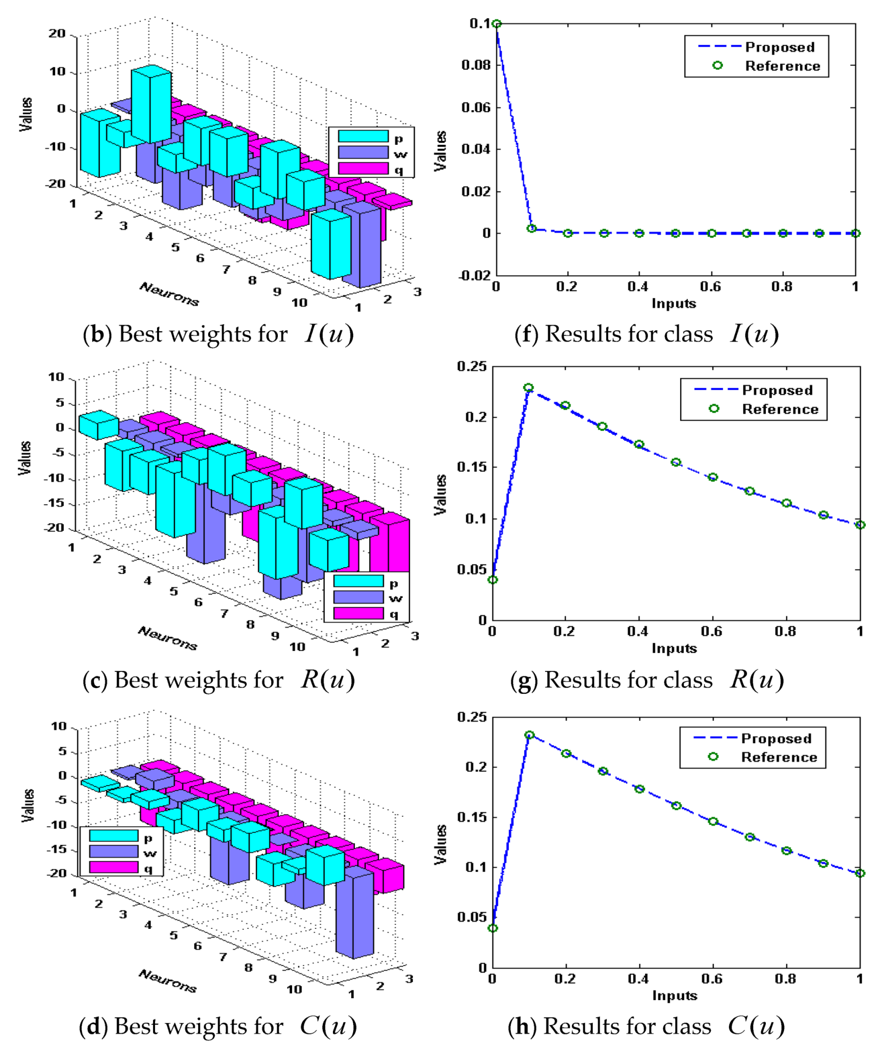
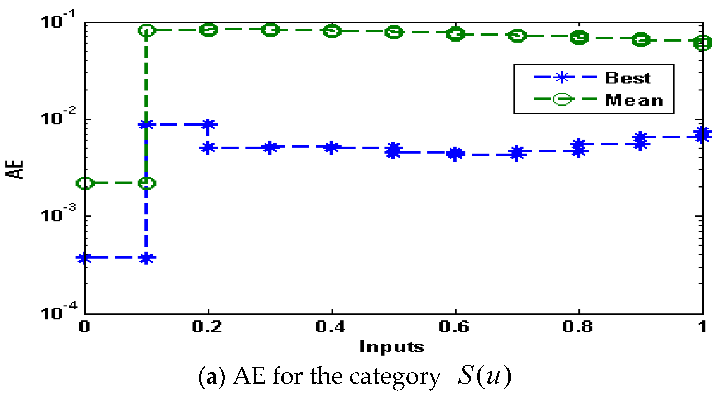
3. Simulations and Results

The relative presentations of the results obtained using the Adams method are used to certify or analyze the accuracy of the ANN-GA-ASM. Moreover, the statistical performance is testified for the precision, reliability and accuracy of the proposed structure. The updated form of the nonlinear model of influenza illness using the appropriate parameters as defined in reported study [13]:

{\begin{cases} S^{'} (u) = 0.02 - (50 I (u) + 0.02) S (u) + 0.5 C (u), & S (0) = 0.8, \\ I^{'} (u) = 50 (S (t) + 0.05 C (u)) I (u) - 73.02 I (u), & I (0) = 0.1, \\ R^{'} (u) = 73 I (u) + 47.5 C (u) I (u) - 1.02 R (u), & R (0) = 0.04, \\ C^{'} (u) = R (u) - (0.52 + 50 I (u)) C (u), & C (0) = 0.06, \end{cases}

(10)

The fitness function for the influenza disease system (10) becomes:

\begin{array}{l} E = \frac{1}{N} \sum_{i = 1}^{N} (\begin{array}{l} {[{\hat{S}}_{i}^{'} - 0.02 + 50 {\hat{S}}_{i} {\hat{I}}_{i} + 0.02 {\hat{S}}_{i} - 0.5 {\hat{C}}_{i}]}^{2} \\ + {[{\hat{I}}_{i}^{'} - 50 {\hat{S}}_{i} {\hat{I}}_{i} - 2.5 {\hat{C}}_{i} {\hat{I}}_{i}_{i} + 73.02 {\hat{I}}_{i}]}^{2} \\ + {[{\hat{R}}_{i}^{'} - 73 {\hat{I}}_{i} - 47.5 {\hat{C}}_{i} {\hat{I}}_{i} + 1.02 {\hat{R}}_{i}]}^{2} \\ + {[{\hat{C}}_{i}^{'} - {\hat{R}}_{i} + 0.52 {\hat{C}}_{i} - 50 {\hat{I}}_{i} {\hat{C}}_{i}]}^{2} \end{array}) \\ + \frac{1}{4} [{({\hat{S}}_{0} - 0.8)}^{2} + {({\hat{I}}_{0} - 0.1)}^{2} + {({\hat{R}}_{0} - 0.04)}^{2} + {({\hat{C}}_{0} - 0.06)}^{2}] . \end{array}

(11)

Performance by optimization is demonstrated for the nonlinear influenza disease model using the proposed ANN-GA-ASM for 30 independent runs, i.e., sufficiently large multiple autonomous executions, having 30 numbers of hidden neurons in ANN models in set (3). The routine for the fitness function as given in Equations (4)–(9) is developed in the Matlab software package while the optimization is conducted as per procedure of pseudocode in Table 1 using the ‘GA’ and ‘fmincon’ routines of the optimization toolbox. The proposed solutions of the nonlinear influenza disease model are specified in the best weight vector form shown in the Equations (12)–(15) for each nonlinear influenza disease model. The graphical illustrations of these weight vectors are shown in Figure 2.

\hat{S} (u) = \frac{0.6622}{1 + e^{- (- 10.636 u - 1.1152)}} - \frac{1.3369}{1 + e^{- (- 3.6682 u - 7.9483)}} - \dots + \frac{0.3752}{1 + e^{- (- 0.096 u - 4.1269)}},

(12)

\hat{I} (u) = \frac{- 14.9676}{1 + e^{- (0.7029 u - 16.7745)}} - \frac{4.1637}{1 + e^{- (- 15.649 u - 16.512)}} - \dots - \frac{15.4637}{1 + e^{- (- 19.7976 u - 1.1137)}},

(13)

\hat{R} (u) = \frac{3.2898}{1 + e^{- (- 1.6034 u - 7.6633)}} - \frac{1.6034}{1 + e^{- (- 8.138 u - 11.8697)}} - \dots - \frac{6.3094}{1 + e^{- (- 1.456 u - 10.9883)}},

(14)

C (u) = \frac{- 0.8800}{1 + e^{- (0.4167 u - 11.3515)}} - \frac{0.8127}{1 + e^{- (- 0.8127 u - 11.351)}} - \dots - \frac{5.8006}{1 + e^{- (- 16.500 u - 4.6960)}} .

(15)

The proposed outputs are obtained using the above systems ((12)–(15)) as provided in Appendix C for the 0–1 range with a 0.1 step size to present the solutions for each influenza disease category. The plots of the best weight vectors are derived in the Figure 2a–d. The mean and best results, i.e., the outcomes of the proposed methodology based on the average and best fitted weights of ANNs, compared with the reference solutions, i.e., the outcomes of the systems calculated with the Adams numerical technique, to get the nonlinear influenza disease models are also plotted in Figure 2e–h. The solutions obtained by the ANN-GA-ASM coincided with the Adams solutions to present the solutions for each category of influenza disease. These results are consistent with the perfection and precision of the proposed ANN-GA-ASM. Figure 3 shows the AE values to provide solutions for each influenza category. One may observe that the AE best values for the susceptible (S), infectious (I), recovered (R) and cross-immune (C) groups based on the influenza disease model lie in the ranges of 10⁻²–10⁻⁴, 10⁻³–10⁻⁶, 10⁻²–10⁻⁴ and 10⁻²–10⁻⁴, respectively. Meanwhile, the AE mean values for the above categories of susceptible, infectious, recovered and cross-immune lie around 10⁻¹–10⁻³, 10⁻²–10⁻⁴, 10⁻¹–10⁻³ and 10⁻¹–10⁻², respectively. Figure 4 represents the performances based on the EVAF, MAD and TIC operators to solve each category of the influenza disease nonlinear model. It is designated that the best EVAF, MAD and TIC presentations of the susceptible category lie around 10⁻²–10⁻⁴, 10⁻²–10⁻³ and 10⁻⁶–10⁻⁸ for EVAF, MAD and TIC, respectively. The infectious best category lies in the range of 10⁻²–10⁻⁴, 10⁻³–10⁻⁴ and 10⁻⁷–10⁻⁸ for EVAF, MAD and TIC, respectively. The recovered best category lies in the range of 10⁻³–10⁻⁴, 10⁻²–10⁻³ and 10⁻⁶–10⁻⁸ for EVAF, MAD and TIC, respectively. The cross-immune best category lies in the range of 10⁻²–10⁻⁴, 10⁻²–10⁻³ and 10⁻⁷–10⁻⁸ for EVAF, MAD and TIC, respectively. These indications make it possible to affirm that the designed ANN-GA-ASM is precise and accurate.

The graphical representations based on the statistical procedures to authenticate the convergence performance are given in Figure 5 to solve the nonlinear influenza disease model. In the performance through TIC values using thirty trials to solve the nonlinear influenza disease model, it is seen that most of the trials based on the susceptible, infectious, recovered and cross-immune for the TIC values lie around 10⁻⁵–10⁻⁷, 10⁻⁶–10⁻⁸, 10⁻⁵–10⁻⁸ and 10⁻⁵–10⁻⁷, respectively. For the EVAF values, the performances of the susceptible, infectious, recovered and cross-immune lie around 10⁻¹–10⁻³. For the MAD values, the performances of the susceptible, infectious, recovered and cross-immune lie around 10⁻²–10⁻⁴. These best presentations of the executions using the ANN-GA-ASM are calculated as suitable for the TIC, EVAF and MAD operators.

The statistical presentations are shown in Table 2, Table 3, Table 4 and Table 5 using the operators Minimum (Min), Mean, standard deviation (SD), S.I.R, Median (Med) and Maximum (Max) to validate the accurateness and precision for solving each category of the influenza disease nonlinear model. The Min values for the susceptible, infectious, recovered and cross-immune based influenza disease model lie around 10⁻³–10⁻⁵, 10⁻³–10⁻⁷, 10⁻³–10⁻⁶ and 10⁻³–10⁻⁵, respectively. The Max values for the susceptible, infectious, recovered and cross-immune based influenza disease model lie around 10⁻¹–10⁻³, 10⁻²–10⁻⁴, 10⁻¹–10⁻² and 10⁻²–10⁻³, respectively. The Med, Mean and S.I.R values for the susceptible, infectious, recovered and cross-immune based influenza disease model lie around 10⁻²–10⁻⁴, 10⁻²–10⁻⁵, 10⁻²–10⁻⁴ and 10⁻³–10⁻⁴, respectively. The SD values for the susceptible, infectious, recovered and cross-immune based influenza disease model lie around 10⁻²–10⁻³, 10⁻²–10⁻⁴, 10⁻²–10⁻³ and 10⁻²–10⁻⁴, respectively. These calculated small values indicate the worth of the ANN-GA-ASM to solve each class of the nonlinear influenza disease model. One can observe through these obtained measures that the designed ANN-GA-ASM is precise, accurate and stable.

The global performances of (G-TIC), (G-MAD) and (G-EVAF) operators for 30 trials to solve the proposed ANN-GA-ASM is shown in Table 6 to solve the nonlinear influenza disease model. These global MAD, TIC and EVAF performances based on Min lie around 10⁻²–10⁻³, 10⁻⁶–10⁻⁷ and 10⁻¹–10⁻², respectively, while the global performances based on S.I.R lie around 10⁻² to 10⁻³, 10⁻⁷–10⁻⁸ and 10⁻¹–10⁻² for each category of the influenza disease nonlinear model. These close ideal values obtained through global measures indicate the precision, correctness and accuracy of the designed ANN-GA-ASM.

4. Conclusions

This study is associated with the submission of numerical studies of the non-linear influenza disease system. The influenza disease nonlinear system is dependent on four categories named as susceptible, infected, recovered and cross-immune. Artificial neural networks, as well as global and local research approaches, i.e., ANN-GA-ASM, are proposed to address each category of the influenza illness model. For finding numeric results, an objective function based on the differential system and initial conditions is optimized by the proposed ANN-GA-ASM. The log-sigmoid works as an activation function and 30 numbers of variables have been proposed to solve the influenza disease nonlinear model. The obtained numerical results through ANN-GA-ASM have been compared with the Adams solutions and the matching of the best/mean results have been found in each class of the nonlinear influenza disease model. The accurate matching of results enhances the reliability of the proposed ANN-GA-ASM. The precise performance of the ANN-GA-ASM through the statistical operators EVAF, TIC and MAD are observed using 30 runs to solve the nonlinear model of influenza disease. These statistical performances achieved higher accuracy levels to solve the influenza disease nonlinear model. Statistics by Min, SD, Mean, S.I.R, Max and Median further validate the value of the proposed ANN-GA-ASM. Furthermore, the global performance of the operators in good measures through Min and S.I.R prove the authenticity of the ANN-GA-ASM for the nonlinear influenza disease model.

In the future, the ANN proposed with the GA-ASM is capable of solving nonlinear biological models, singular systems of higher order and fluid dynamics models. Moreover, the provided ANN-GA-ASM can be implemented to those problems which are still considered to be stiff for traditional deterministic computing schemes.

Author Contributions

Writing—original draft preparation, Z.S.; Funding acquisition, A.A.A.I.; writing—review and editing, M.A.Z.R.; Administration, K.N.; Formal analysis, M.U.; Validation, J.J.P.C.R.; Supervision, S.R.M. All authors have read and agreed to the published version of the manuscript.

Funding

The manuscript APC is supported by Universiti Malaysia Sabah, Jalan UMS, 88400, KK, Malaysia. Furthermore, this work is partially funded by FCT/MCTES through national funds and when applicable co-funded EU funds under the Project UIDB/50008/2020; and by Brazilian National Council for Scientific and Technological Development-CNPq, via Grant No. 313036/2020-9.

Institutional Review Board Statement

Not applicable.

Informed Consent Statement

Not applicable.

Data Availability Statement

Not applicable.

Conflicts of Interest

All authors of the manuscript declare that there have no potential conflicts of interest.

Nomenclature

ANN	Artificial Neural Networks
SIQR	Susceptible–infectious–quarantine–recovered
(SITR)	Susceptible–infectious–treatment–recovered
ANN-GA-ASM-	ANN optimized with GA-ASM
TIC	‘Theil’s inequality coefficient
S.I.R	Semi interquartile
Min	Minimum
Med	Median
G.MAD	Mean of MAD
GA	Genetic Algorithms
ASM	Active-set Algorithm
GA-ASM	Hybrid of GA and ASM
MAD	Mean Absolute deviation
VAF	Variance account for
EVAF	Error in VAF
Max	Maximum
G.TIC	Mean of TIC
G.EVAF	Mean of EVAF

Appendix A

The updated form of the networks as given in set of Equation (2) using the log-sigmoid function are given as follows:

[\hat{S} (u), \hat{I} (u), \hat{R} (u), \hat{C} (u)] = [\begin{array}{l} \sum_{k = 1}^{m} \frac{p_{S, k}}{1 + e^{- (w_{S, k} u + q_{P, k})}}, \sum_{k = 1}^{m} \frac{p_{I, k}}{1 + e^{- (w_{I, k} u + q_{I, k})}}, \\ \sum_{k = 1}^{m} \frac{p_{R, k}}{1 + e^{- (w_{R, k} u + q_{R, k})}}, \sum_{k = 1}^{m} \frac{p_{_{C}, k}}{1 + e^{- (w_{C, k} u + q_{C, k})}}, \end{array}], [{\hat{S}}^{'} (u), {\hat{I}}^{'} (u), {\hat{R}}^{'} (u), {\hat{C}}^{'} (u)] = [\begin{array}{l} \sum_{k = 1}^{m} \frac{w_{S, k} p_{S, k} e^{- (w_{S, k} u + q_{S, k})}}{{(1 + e^{- (w_{P, k} u + q_{P, k})})}^{2}}, \sum_{i = 1}^{m} \frac{w_{I, k} p_{I, k} e^{- (w_{I, k} u + q_{I, k})}}{{(1 + e^{- (w_{I, k} u + q_{I, k})})}^{2}}, \\ \sum_{k = 1}^{m} \frac{w_{R, k} p_{R, k} e^{- (w_{R, k} u + q_{R, k})}}{{(1 + e^{- (w_{R, k} u + q_{R, k})})}^{2}}, \sum_{k = 1}^{m} \frac{w_{_{C}, k} p_{_{C}, k} e^{- (w_{C, k} u + q_{C, k})}}{{(1 + e^{- (w_{C, k} u + q_{C, k})})}^{2}} \end{array}] .

(A1)

Appendix B

Mathematical relations for performance indices TIC, MAD, VAF and EVAF are given in this section as follows:

{\begin{cases} {[VAF}_{S}, {VAF}_{I}, {VAF}_{R}, {VAF}_{C}] = [\begin{array}{l} (1 - \frac{var (S_{i} - {\hat{S}}_{i})}{var (S_{i})}) \times 100, \\ (1 - \frac{var (I_{i} - {\hat{I}}_{i})}{var (S_{i})}) \times 100, \\ (1 - \frac{var (I_{i} - {\hat{I}}_{i})}{var (I_{i})}) \times 100, \\ (1 - \frac{var (R_{i} - {\hat{R}}_{i})}{var (R_{i})}) \times 100 \end{array}], \\ {[EVAF}_{S}, {EVAF}_{p}, {EVAF}_{R}, {EVAF}_{R}] = [| \begin{array}{l} 100 - {VAF}_{S}, 100 - {VAF}_{I}, \\ 100 - {VAF}_{_{R}}, 100 - {VAF}_{_{C}} \end{array} |] . \end{cases}

(A2)

{\begin{cases} S . I . R = - \frac{1}{2} (Q_{1} - Q_{3}), \\ Q_{1} = 1^{s t} quartile & Q_{3} = 3^{r d} quartile, \end{cases}

(A3)

[{TIC}_{S}, {TIC}_{I}, {TIC}_{R}, {TIC}_{c}] = [\begin{array}{l} \frac{\sqrt{\frac{1}{n} {\sum_{i = 1}^{n} (S_{i} - {\hat{S}}_{i})}^{2}}}{(\sqrt{\frac{1}{n} \sum_{i = 1}^{n} S_{i}^{2}} + \sqrt{\frac{1}{n} \sum_{i = 1}^{n} {\hat{S}}^{2}_{i}})}, \frac{\sqrt{\frac{1}{n} {\sum_{i = 1}^{n} (I_{i} - {\hat{I}}_{i})}^{2}}}{(\sqrt{\frac{1}{n} \sum_{i = 1}^{n} I_{i}^{2}} + \sqrt{\frac{1}{n} \sum_{i = 1}^{n} {\hat{I}}_{i}^{2}})}, \\ \frac{\sqrt{\frac{1}{n} {\sum_{i = 1}^{n} (R_{i} - {\hat{R}}_{i})}^{2}}}{(\sqrt{\frac{1}{n} \sum_{i = 1}^{n} R_{i}^{2}} + \sqrt{\frac{1}{n} \sum_{i = 1}^{n} {\hat{R}}_{i}^{2}})}, \frac{\sqrt{\frac{1}{n} {\sum_{r = 1}^{n} (C_{i} - {\hat{C}}_{i})}^{2}}}{(\sqrt{\frac{1}{n} \sum_{i = 1}^{n} C_{i}^{2}} + \sqrt{\frac{1}{n} \sum_{i = 1}^{n} {\hat{C}}_{i}^{2}})} \end{array}],

(A4)

{[MAD}_{S}, {MAD}_{I} {, MAD}_{R} {, MAD}_{C}] = [\begin{array}{l} \sum_{i = 1}^{n} | S_{i} - {\hat{S}}_{i} |, \sum_{i = 1}^{n} | I_{i} - {\hat{I}}_{i} |, \\ \sum_{i = 1}^{n} | R_{i} - {\hat{R}}_{i} |, \sum_{i = 1}^{n} | C_{i} - {\hat{C}}_{i} | \end{array}] .

(A5)

In the above system,

\hat{P}, \hat{S}, {\hat{Q}}_{T}

and

{\hat{Q}}_{S}

show the approximate solutions.

Appendix C

The proposed solutions of ANN-GA-ASM are for reproduction of the results.

\begin{array}{l} \hat{S} (u) & = \frac{0.6622}{1 + e^{- (- 10.636 u - 1.1152)}} - \frac{1.3369}{1 + e^{- (- 3.6682 u - 7.9483)}} - \frac{2.6556}{1 + e^{- (0.553 u - 9.2701)}} - \frac{9.3591}{1 + e^{- (0.034 u + 0.2050)}} \\ - \frac{8.6110}{1 + e^{- (0.0851 u - 9.8015)}} - \frac{7.1545}{1 + e^{- (3.1236 u + 7.8750)}} + \frac{10.4165}{1 + e^{- (- 20 u - 2.1186)}} + \frac{- 8.0870}{1 + e^{- (- 17.6017 u - 1.7998)}} \\ - \frac{1.0581}{1 + e^{- (- 9.987 u - 13.1919)}} + \frac{0.3752}{1 + e^{- (- 0.096 u - 4.1269)}}, \end{array}

(A6)

\begin{array}{l} \hat{I} (u) & = \frac{- 14.9676}{1 + e^{- (0.7029 u - 16.7745)}} - \frac{4.1637}{1 + e^{- (- 15.649 u - 16.512)}} - \frac{17.5790}{1 + e^{- (- 19.755 u - 1.2481)}} - \frac{4.8989}{1 + e^{- (- 10.5358 u - 10.12)}} \\ + \frac{9.9541}{1 + e^{- (- 13.11 u - 19.305)}} - \frac{10.1789}{1 + e^{- (- 13.342 u - 18.201)}} - \frac{5.6472}{1 + e^{- (- 10.7019 u - 8.831)}} + \frac{12.4043}{1 + e^{- (- 5.4385 u - 13.809)}} \\ + \frac{7.5788}{1 + e^{- (- 9.905 u - 13.476)}} - \frac{15.4637}{1 + e^{- (- 19.7976 u - 1.1137)}}, \end{array}

(A7)

\begin{array}{l} \hat{R} (u) & = \frac{3.2898}{1 + e^{- (- 1.6034 u - 7.6633)}} - \frac{1.6034}{1 + e^{- (- 8.138 u - 11.8697)}} - \frac{6.47733}{1 + e^{- (- 0.6671 u - 13.6916)}} - \frac{12.8102}{1 + e^{- (- 19.583 u - 1.9607)}} \\ + \frac{4.8765}{1 + e^{- (- 7.6164 u - 14.717)}} - \frac{7.9570}{1 + e^{- (- 2.311 u - 11.1267)}} - \frac{4.7964}{1 + e^{- (- 20.00 u - 0.9233)}} - \frac{- 12.2337}{1 + e^{- (- 14.431 u - 14.7060)}} \\ + \frac{7.8623}{1 + e^{- (- 1.0326 u - 3.398)}} - \frac{6.3094}{1 + e^{- (- 1.456 u - 10.9883)}}, \end{array}

(A8)

\begin{array}{l} C (u) & = \frac{- 0.8800}{1 + e^{- (0.4167 u - 11.3515)}} - \frac{0.8127}{1 + e^{- (- 0.8127 u - 11.351)}} - \frac{1.6459}{1 + e^{- (- 2.280 u - 7.6613)}} - \frac{2.7450}{1 + e^{- (- 1.5173 u - 3.2116)}} \\ - \frac{4.3108}{1 + e^{- (- 12.4865 u - 3.8263)}} + \frac{2.4976}{1 + e^{- (- 0.1237 u - 7.3027)}} + \frac{3.9922}{1 + e^{- (0.0154 u - 3.1261)}} - \frac{4.6329}{1 + e^{- (- 10.73 u - 3.4104)}} \\ - \frac{1.1761}{1 + e^{- (- 0.8082 u - 8.0611)}} - \frac{5.8006}{1 + e^{- (- 16.500 u - 4.6960)}} . \end{array}

(A9)

References

World Health Organization (WHO). Influenza Overview. Available online: http://www.who.int/mediacentre/factsheets/fs211/en/ (accessed on 16 May 2021).
Astuti, F.; Suryanto, A.; Darti, I. Multi-step differential transform method for solving the influenza virus model with disease resistance. IOP Conf. Ser. Mater. Sci. Eng. 2019, 546, 052013. [Google Scholar] [CrossRef]
Erdem, M.; Safan, M.; Castillo-Chavez, C. Mathematical analysis of an SIQR influenza model with imperfect quarantine. Bull. Math. Biol. 2017, 79, 1612–1636. [Google Scholar] [CrossRef] [PubMed]
Alzahrani, E.O.; Khan, M.A. Comparison of numerical techniques for the solution of a fractional epidemic model. Eur. Phys. J. Plus 2020, 135, 110. [Google Scholar] [CrossRef]
Sun, L.; DePuy, G.W.; Evans, G.W. Multi-objective optimization models for patient allocation during a pandemic influenza outbreak. Comput. Oper. Res. 2014, 51, 350–359. [Google Scholar] [CrossRef]
Ghanbari, B.; Gómez-Aguilar, J.F. Analysis of two avian influenza epidemic models involving fractal-fractional derivatives with power and Mittag-Leffler memories. Chaos Interdiscip. J. Nonlinear Sci. 2019, 29, 123113. [Google Scholar] [CrossRef] [PubMed]
Arenas, A.J.; González-Parra, G.; Chen-Charpentier, B.M. Construction of nonstandard finite difference schemes for the SI and SIR epidemic models of fractional order. Math. Comput. Simul. 2016, 121, 48–63. [Google Scholar] [CrossRef]
Tchuenche, J.M.; Dube, N.; Bhunu, C.P.; Smith, R.J.; Bauch, C.T. The impact of media coverage on the transmission dynamics of human influenza. BMC Public Health 2011, 11, S5. [Google Scholar] [CrossRef] [Green Version]
Schulze-Horsel, J.; Schulze, M.; Agalaridis, G.; Genzel, Y.; Reichl, U. Infection dynamics and virus-induced apoptosis in cell culture-based influenza vaccine production—Flow cytometry and mathematical modeling. Vaccine 2009, 27, 2712–2722. [Google Scholar] [CrossRef]
Hovav, S.; Tsadikovich, D. A network flow model for inventory management and distribution of influenza vaccines through a healthcare supply chain. Oper. Res. Health Care 2015, 5, 49–62. [Google Scholar] [CrossRef]
Patel, R.; Longini, I.M.; Halloran, M.E. Finding optimal vaccination strategies for pandemic influenza using genetic algorithms. J. Theor. Biol. 2005, 234, 201–212. [Google Scholar] [CrossRef]
Kanyiri, C.W.; Luboobi, L.; Kimathi, M. Application of optimal control to influenza pneumonia coinfection with antiviral resistance. Comput. Math. Methods Med. 2020, 2020, 5984095. [Google Scholar] [CrossRef]
Jódar, L.; Villanueva, R.J.; Arenas, A.J.; González, G.C. Nonstandard numerical methods for a mathematical model for influenza disease. Math. Comput. Simul. 2008, 79, 622–633. [Google Scholar] [CrossRef]
Casagrandi, R.; Bolzoni, L.; Levin, S.A.; Andreasen, V. The SIRC model and influenza A. Math. Biosci. 2006, 200, 152–169. [Google Scholar] [CrossRef]
Zachreson, C.; Fair, K.M.; Harding, N.; Prokopenko, M. Interfering with influenza: Nonlinear coupling of reactive and static mitigation strategies. J. R. Soc. Interface 2020, 17, 20190728. [Google Scholar] [CrossRef] [PubMed] [Green Version]
Jiang, X.; Yu, Y.; Meng, F.; Xu, Y. Modelling the dynamics of avian influenza with nonlinear recovery rate and psychological effect. J. Appl. Anal. Comput. 2020, 10, 1170–1192. [Google Scholar] [CrossRef]
Chong, K.C.; Liang, J.; Jia, K.M.; Kobayashi, N.; Wang, M.H.; Wei, L.; Lau, S.Y.F.; Sumi, A. Latitudes mediate the association between influenza activity and meteorological factors: A nationwide modelling analysis in 45 Japanese prefectures from 2000 to 2018. Sci. Total Environ. 2020, 703, 134727. [Google Scholar] [CrossRef] [PubMed]
Handel, A.; Liao, L.E.; Beauchemin, C.A. Progress and trends in mathematical modelling of influenza A virus infections. Curr. Opin. Syst. Biol. 2018, 12, 30–36. [Google Scholar] [CrossRef]
McCarthy, Z.; Athar, S.; Alavinejad, M.; Chow, C.; Moyles, I.; Nah, K.; Kong, J.D.; Agrawal, N.; Jaber, A.; Keane, L.; et al. Quantifying the annual incidence and underestimation of seasonal influenza: A modelling approach. Theor. Biol. Med Model. 2020, 17, 11. [Google Scholar] [CrossRef] [PubMed]
Sabir, Z.; Raja, M.A.Z.; Baleanu, D. Fractional mayer neuro-swarm heuristic solver for multi-fractional order doubly singular model based on lane–emden equation. Fractals 2021, 29, 2040033. [Google Scholar]
Umar, M.; Sabir, Z.; Raja, M.A.Z.; Shoaib, M.; Gupta, M.; Sánchez, Y.G. A stochastic intelligent computing with neuro-evolution heuristics for nonlinear SITR system of novel COVID-19 dynamics. Symmetry 2020, 12, 1628. [Google Scholar] [CrossRef]
Tao, Z.; Huiling, L.; Wenwen, W.; Xia, Y. GA-SVM based feature selection and parameter optimization in hospitalization expense modeling. Appl. Soft Comput. 2019, 75, 323–332. [Google Scholar] [CrossRef]
Sayed, S.; Nassef, M.; Badr, A.; Farag, I. A Nested Genetic Algorithm for feature selection in high-dimensional cancer Microarray datasets. Expert Syst. Appl. 2019, 121, 233–243. [Google Scholar] [CrossRef]
Hemanth, D.J.; Anitha, J. Modified Genetic Algorithm approaches for classification of abnormal Magnetic Resonance Brain tumour images. Appl. Soft Comput. 2019, 75, 21–28. [Google Scholar] [CrossRef]
Armaghani, D.J.; Hasanipanah, M.; Mahdiyar, A.; Majid, M.Z.A.; Amnieh, H.B.; Tahir, M.M.D. Airblast prediction through a hybrid genetic algorithm-ANN model. Neural Comput. Appl. 2018, 29, 619–629. [Google Scholar] [CrossRef]
Jiang, Y.; Wu, P.; Zeng, J.; Zhang, Y.; Zhang, Y.; Wang, S. Multi-parameter and multi-objective optimisation of articulated monorail vehicle system dynamics using genetic algorithm. Veh. Syst. Dyn. 2019, 58, 74–91. [Google Scholar] [CrossRef]
Yang, Y.; Yang, B.; Wang, S.; Liu, F.; Wang, Y.; Shu, X. A dynamic ant-colony genetic algorithm for cloud service composition optimization. Int. J. Adv. Manuf. Technol. 2019, 102, 355–368. [Google Scholar] [CrossRef]
Hassoon, M.; Kouhi, M.S.; Zomorodi-Moghadam, M.; Abdar, M. Rule optimization of boosted C5.0 classification using genetic algorithm for liver disease prediction. In Proceedings of the 2017 International Conference on Computer and Applications (ICCA), Doha, Qatar, 6–7 September 2017; pp. 299–305. [Google Scholar]
Quirynen, R.; Knyazev, A.; Di Cairano, S. Block structured preconditioning within an active-set method for real-time optimal control. In Proceedings of the 2018 European Control Conference (ECC), Limassol, Cyprus, 12–15 June 2018; pp. 1154–1159. [Google Scholar]
Gao, Y.; Song, H.; Wang, X.; Zhang, K. Primal-dual active set method for pricing American better-of option on two assets. Commun. Nonlinear Sci. Numer. Simul. 2020, 80, 104976. [Google Scholar] [CrossRef]
Deuerlein, J.W.; Piller, O.; Elhay, S.; Simpson, A.R. Content-based active-set method for the pressure-dependent model of water distribution systems. J. Water Resour. Plan. Manag. 2019, 145, 04018082. [Google Scholar] [CrossRef] [Green Version]
Swathika, O.V.G.; Das, A.; Gupta, Y.; Mukhopadhyay, S.; Hemamalini, S.; Satapathy, S.C.; Bhateja, V.; Udgata, S.K.; Pattnaik, P.K. Optimization of overcurrent relays in microgrid using interior point method and active set method. In Proceedings of the Advances in Intelligent Systems and Computing; Springer Science and Business Media LLC: Singapore, 2017; Volume 516, pp. 89–97. [Google Scholar]
Klaučo, M.; Kalúz, M.; Kvasnica, M. Machine learning-based warm starting of active set methods in embedded model predictive control. Eng. Appl. Artif. Intell. 2019, 77, 1–8. [Google Scholar] [CrossRef]
Abide, S.; Barboteu, M.; Cherkaoui, S.; Danan, D.; Dumont, S. Inexact primal–dual active set method for solving elastodynamic frictional contact problems. Comput. Math. Appl. 2021, 82, 36–59. [Google Scholar] [CrossRef]

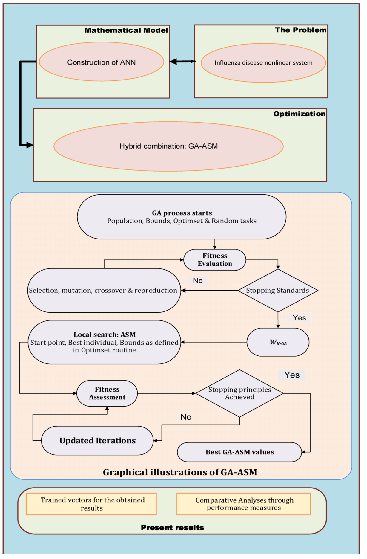
Figure 1. Proposed structure of the present ANN-GA-ASM for solving the nonlinear influenza disease model.

Figure 2. Best set of weight vectors and comparison of proposed and reference solutions obtained by using Adams and optimization algorithm to solve the influenza nonlinear disease model.

Figure 3. AE values based on best and mean solutions for each category of the influenza disease nonlinear model.

Figure 4. Performances of EVAF, MAD and TIC operators to solve the influenza disease model.

Figure 5. Convergence operators based on TIC, EVAF and MAD operators to solve the nonlinear influenza disease model.

Table 1. Pseudocode of optimization through ANN-GA-ASM to solve the influenza disease nonlinear system.

GA process starts

Inputs: Select the chromosomes with the same numbers as decision variable of

ANN models for solving influenza disease system:

W = [a, w, b]

Population: The chromosomes set is given as:

W = [W_{S}, W_{I}, W_{R}, W_{C}]

, for

W_{S} = [p_{S}, ω_{S}, q_{S}]

,

W_{I} = [p_{I}, ω_{I}, q_{I}]

,

W_{R} = [p_{R}, ω_{R}, q_{R}]

and

W_{R} = [p_{R}, ω_{R}, q_{R}]

Output: Global vectors are W_B-GA

Initialization: For variables selection, modify the weight vector.

Fitness calculation: Determine the fitness E of each member of the population

(P) using Equations (4)–(9)

• Stopping standards: Terminate if [E = 10⁻²¹], [TolCon = TolFun = 10⁻²¹].

[StallLimit = 140], [PopSize = 210] and [Generations = 120] are achieved.

Move to storage

Ranking: Rank precise weight vector in the designated population based on

appropriateness on fitness E, i.e., better the fitness more be the rank of the

individual.

Storage: Save W_B-GA, iterations, FIT, function counts and time.

End of GA

ASM

Inputs: W_B-GA.

Output: W_GA-ASM is the best GA-ASM weight vectors.

Initialize: W_B-GA, iterations, assignments and other values.

Termination: Stop if [E = 10⁻²⁰], [Iterations = 1200], [TolX = TolCon = 10⁻²⁰]

[TolFun = 10⁻²¹] and [MaxFunEvals = 279,000] meets.

Evaluation of FIT: Calculate W and E using networks 4–9.

Adjustments: Adjust ‘fmincon’ for ASM, calculate E using 4–9 systems.

Accumulate: Transmute W_GA-ASM, function counts, time iterations and FIT

ASM End

Table 2. Statistical measures for the nonlinear influenza disease model based

S (u)

.

Table 2. Statistical measures for the nonlinear influenza disease model based

S (u)

.

$u$	$S (u)$
$u$	Min	Max	Med	Mean	S.I.R	SD
0	5.6403 × 10⁻⁵	1.0752 × 10⁻²	6.4347 × 10⁻⁴	2.1832 × 10⁻³	9.2647 × 10⁻⁴	3.1586 × 10⁻³
0.1	8.6933 × 10⁻³	1.0204 × 10⁻¹	9.9764 × 10⁻²	8.0571 × 10⁻²	1.7817 × 10⁻²	3.2865 × 10⁻²
0.2	5.0136 × 10⁻³	1.0330 × 10⁻¹	1.0171 × 10⁻²	8.2758 × 10⁻²	1.5101 × 10⁻²	3.3698 × 10⁻²
0.3	5.0721 × 10⁻³	1.0168 × 10⁻¹	1.0031 × 10⁻²	8.1157 × 10⁻²	1.3434 × 10⁻²	3.3551 × 10⁻²
0.4	4.9908 × 10⁻³	1.0007 × 10⁻¹	9.6958 × 10⁻²	7.9023 × 10⁻²	1.2838 × 10⁻²	3.2084 × 10⁻²
0.5	4.4433 × 10⁻³	9.7345 × 10⁻²	9.3189 × 10⁻²	7.6406 × 10⁻²	1.2362 × 10⁻²	3.0706 × 10⁻²
0.6	4.2461 × 10⁻³	9.3883 × 10⁻²	9.0095 × 10⁻²	7.3296 × 10⁻²	1.2040 × 10⁻²	2.9743 × 10⁻²
0.7	4.6397 × 10⁻³	8.9911 × 10⁻²	8.6530 × 10⁻²	6.9938 × 10⁻²	1.1763 × 10⁻²	2.8846 × 10⁻²
0.8	5.4428 × 10⁻³	8.5574 × 10⁻²	8.2248 × 10⁻²	6.6416 × 10⁻²	1.1654 × 10⁻²	2.7814 × 10⁻²
0.9	6.3978 × 10⁻³	8.0976 × 10⁻²	7.8024 × 10⁻²	6.2713 × 10⁻²	1.1469 × 10⁻²	2.6591 × 10⁻²
1	7.3410 × 10⁻³	7.6194 × 10⁻²	7.3517 × 10⁻²	5.8825 × 10⁻²	1.1127 × 10⁻²	2.5110 × 10⁻²

Table 3. Statistical measures for the nonlinear influenza disease model based

I (u)

.

Table 3. Statistical measures for the nonlinear influenza disease model based

I (u)

.

$u$	$I (u)$
$u$	Min	Max	Med	Mean	S.I.R	SD
0	2.5065 × 10⁻³	9.9741 × 10⁻²	9.6765 × 10⁻²	2.1832 × 10⁻³	1.8123 × 10⁻²	3.2534 × 10⁻²
0.1	2.0358 × 10⁻⁴	3.8280 × 10⁻³	2.6376 × 10⁻³	8.0571 × 10⁻²	2.9036 × 10⁻⁴	7.8410 × 10⁻⁴
0.2	1.0562 × 10⁻⁴	1.5922 × 10⁻³	2.8609 × 10⁻⁴	8.2758 × 10⁻²	9.2734 × 10⁻⁵	3.2756 × 10⁻⁴
0.3	7.9627 × 10⁻⁶	7.5276 × 10⁻⁴	1.4348 × 10⁻⁴	8.1157 × 10⁻²	1.0830 × 10⁻⁴	1.7174 × 10⁻⁴
0.4	5.8824 × 10⁻⁶	1.1768 × 10⁻³	1.4911 × 10⁻⁴	7.9023 × 10⁻²	6.2778 × 10⁻⁵	2.5473 × 10⁻⁴
0.5	5.2022 × 10⁻⁷	8.4523 × 10⁻⁴	8.5497 × 10⁻⁵	7.6406 × 10⁻²	5.2659 × 10⁻⁵	1.7651 × 10⁻⁴
0.6	3.9676 × 10⁻⁷	9.6438 × 10⁻⁴	6.6933 × 10⁻⁵	7.3296 × 10⁻²	5.8891 × 10⁻⁵	1.9772 × 10⁻⁴
0.7	1.4420 × 10⁻⁶	1.0347 × 10⁻³	8.1183 × 10⁻⁵	6.9938 × 10⁻²	5.7567 × 10⁻⁵	2.2108 × 10⁻⁴
0.8	1.3782 × 10⁻⁶	1.0473 × 10⁻³	6.5095 × 10⁻⁵	6.6416 × 10⁻²	5.3914 × 10⁻⁵	1.9876 × 10⁻⁴
0.9	1.0788 × 10⁻⁶	9.9345 × 10⁻⁴	6.9847 × 10⁻⁵	6.2713 × 10⁻²	4.8355 × 10⁻⁵	1.8417 × 10⁻⁴
1	3.7397 × 10⁻⁷	8.6629 × 10⁻⁴	6.3295 × 10⁻⁵	5.8825 × 10⁻²	3.6254 × 10⁻⁵	1.5961 × 10⁻⁴

Table 4. Statistical measures for the nonlinear influenza disease model based

R (u)

.

Table 4. Statistical measures for the nonlinear influenza disease model based

R (u)

.

$u$	$R (u)$
$u$	Min	Max	Med	Mean	S.I.R	SD
0	6.2366 × 10⁻⁶	1.4851 × 10⁻²	1.8505 × 10⁻⁴	2.1832 × 10⁻³	3.8502 × 10⁻⁴	2.9318 × 10⁻³
0.1	2.4607 × 10⁻³	1.9038 × 10⁻¹	1.8634 × 10⁻¹	8.0571 × 10⁻²	3.2715 × 10⁻²	6.2894 × 10⁻²
0.2	2.3532 × 10⁻³	1.7746 × 10⁻¹	1.7489 × 10⁻¹	8.2758 × 10⁻²	2.4669 × 10⁻²	5.9498 × 10⁻²
0.3	2.3392 × 10⁻³	1.6039 × 10⁻¹	1.5817 × 10⁻¹	8.1157 × 10⁻²	2.0756 × 10⁻²	5.4314 × 10⁻²
0.4	1.7447 × 10⁻³	1.4608 × 10⁻¹	1.4106 × 10⁻¹	7.9023 × 10⁻²	1.8914 × 10⁻²	4.8288 × 10⁻²
0.5	1.4329 × 10⁻³	1.3259 × 10⁻¹	1.2623 × 10⁻¹	7.6406 × 10⁻²	1.7328 × 10⁻²	4.3191 × 10⁻²
0.6	6.3834 × 10⁻⁴	1.1983 × 10⁻¹	1.1406 × 10⁻¹	7.3296 × 10⁻²	1.5985 × 10⁻²	3.9221 × 10⁻²
0.7	1.0809 × 10⁻³	1.0806 × 10⁻¹	1.0395 × 10⁻¹	6.9938 × 10⁻²	1.4990 × 10⁻²	3.5981 × 10⁻²
0.8	9.6811 × 10⁻⁴	9.7331 × 10⁻²	9.4041 × 10⁻²	6.6416 × 10⁻²	1.3740 × 10⁻²	3.3132 × 10⁻²
0.9	6.8779 × 10⁻⁴	8.7620 × 10⁻²	8.5302 × 10⁻²	6.2713 × 10⁻²	1.2596 × 10⁻²	3.0469 × 10⁻²
1	3.8749 × 10⁻⁴	7.8853 × 10⁻²	7.7195 × 10⁻²	5.8825 × 10⁻²	1.0930 × 10⁻²	2.7874 × 10⁻²

Table 5. Statistical measures for the nonlinear influenza disease model based

C (u)

.

Table 5. Statistical measures for the nonlinear influenza disease model based

C (u)

.

$u$	$C (u)$
$u$	Min	Max	Med	Mean	S.I.R	SD
0	1.1372 × 10⁻⁵	6.9224 × 10⁻³	2.1165 × 10⁻⁴	1.1227 × 10⁻³	6.5694 × 10⁻⁴	1.8441 × 10⁻³
0.1	1.5570 × 10⁻⁴	1.5199 × 10⁻²	7.0904 × 10⁻³	7.0882 × 10⁻³	3.7494 × 10⁻⁴	2.5091 × 10⁻³
0.2	2.3633 × 10⁻³	2.9209 × 10⁻²	2.4420 × 10⁻²	2.0540 × 10⁻²	4.4120 × 10⁻³	7.6724 × 10⁻³
0.3	2.5936 × 10⁻⁴	4.1491 × 10⁻²	3.9420 × 10⁻²	3.2301 × 10⁻²	7.0413 × 10⁻³	1.3088 × 10⁻²
0.4	1.8337 × 10⁻⁴	5.4041 × 10⁻²	5.1929 × 10⁻²	4.2548 × 10⁻²	8.7280 × 10⁻³	1.7298 × 10⁻²
0.5	1.6757 × 10⁻³	6.4379 × 10⁻²	6.2491 × 10⁻²	5.1205 × 10⁻²	9.0134 × 10⁻³	2.0582 × 10⁻²
0.6	1.7138 × 10⁻³	7.3162 × 10⁻²	7.1056 × 10⁻²	5.8351 × 10⁻²	9.3617 × 10⁻³	2.3249 × 10⁻²
0.7	1.6948 × 10⁻³	8.0311 × 10⁻²	7.8098 × 10⁻²	6.4106 × 10⁻²	9.7669 × 10⁻³	2.5506 × 10⁻²
0.8	1.5227 × 10⁻³	8.6049 × 10⁻²	8.3577 × 10⁻²	6.8593 × 10⁻²	1.0268 × 10⁻²	2.7492 × 10⁻⁴
0.9	1.1457 × 10⁻³	9.0577 × 10⁻²	8.7617 × 10⁻²	7.1938 × 10⁻²	1.0876 × 10⁻²	2.9302 × 10⁻²
1	5.6992 × 10⁻⁴	9.4077 × 10⁻²	9.1159 × 10⁻²	7.4264 × 10⁻²	1.1513 × 10⁻²	3.1009 × 10⁻²

Table 6. Global presentations via G-TIC, G-MAD and G-EVAF operators to solve the nonlinear influenza disease system.

Index	(G-MAD)		(G-TIC)		(G-EVAF)
Index	Min	S.I.R	Min	S.I.R	Min	S.I.R
$S (u)$	8.2308 × 10⁻²	1.1452 × 10⁻²	3.5709 × 10⁻⁶	5.0771 × 10⁻⁷	9.5011 × 10⁻¹	2.7588 × 10⁻¹
$I (u)$	9.1646 × 10⁻³	1.6069 × 10⁻³	1.2032 × 10⁻⁶	2.2481 × 10⁻⁷	9.3349 × 10⁻¹	2.9071 × 10⁻¹
$R (u)$	1.1467 × 10⁻²	1.6332 × 10⁻²	5.1525 × 10⁻⁶	7.5221 × 10⁻⁸	8.7737 × 10⁻¹	2.0805 × 10⁻²
$C (u)$	5.4491 × 10⁻²	7.7396 × 10⁻³	2.5843 × 10⁻⁷	3.4476 × 10⁻⁷	1.0349 × 10⁻²	2.1164 × 10⁻¹

Publisher’s Note: MDPI stays neutral with regard to jurisdictional claims in published maps and institutional affiliations.

© 2021 by the authors. Licensee MDPI, Basel, Switzerland. This article is an open access article distributed under the terms and conditions of the Creative Commons Attribution (CC BY) license (https://creativecommons.org/licenses/by/4.0/).

Share and Cite

MDPI and ACS Style

Sabir, Z.; Ag Ibrahim, A.A.; Raja, M.A.Z.; Nisar, K.; Umar, M.; Rodrigues, J.J.P.C.; Mahmoud, S.R. Soft Computing Paradigms to Find the Numerical Solutions of a Nonlinear Influenza Disease Model. Appl. Sci. 2021, 11, 8549. https://doi.org/10.3390/app11188549

AMA Style

Sabir Z, Ag Ibrahim AA, Raja MAZ, Nisar K, Umar M, Rodrigues JJPC, Mahmoud SR. Soft Computing Paradigms to Find the Numerical Solutions of a Nonlinear Influenza Disease Model. Applied Sciences. 2021; 11(18):8549. https://doi.org/10.3390/app11188549

Chicago/Turabian Style

Sabir, Zulqurnain, Ag Asri Ag Ibrahim, Muhammad Asif Zahoor Raja, Kashif Nisar, Muhammad Umar, Joel J. P. C. Rodrigues, and Samy R. Mahmoud. 2021. "Soft Computing Paradigms to Find the Numerical Solutions of a Nonlinear Influenza Disease Model" Applied Sciences 11, no. 18: 8549. https://doi.org/10.3390/app11188549

Note that from the first issue of 2016, this journal uses article numbers instead of page numbers. See further details here.

Article Menu

Soft Computing Paradigms to Find the Numerical Solutions of a Nonlinear Influenza Disease Model

Abstract

1. Introduction

2. Methodology

2.1. ANN Structure

2.2. Optimization Performances: GA-ASM

2.3. Performance Measures

3. Simulations and Results

4. Conclusions

Author Contributions

Funding

Institutional Review Board Statement

Informed Consent Statement

Data Availability Statement

Conflicts of Interest

Nomenclature

Appendix A

Appendix B

Appendix C

References

Share and Cite

Article Metrics

Article Access Statistics

Further Information

Guidelines

MDPI Initiatives

Follow MDPI