Real-Time Cloth Simulation Using Compute Shader in Unity3D for AR/VR Contents

Featured Application

The proposed method can be applied to represent the cloth object in Unity3D for AR/VR application, interactive game development, force-based deformable object simulation, etc.

Abstract

While the cloth component in Unity engine has been used to represent the 3D cloth object for augmented reality (AR) and virtual reality (VR), it has several limitations in term of resolution and performance. The purpose of our research is to develop a stable cloth simulation based on a parallel algorithm. The method of a mass–spring system is applied to real-time cloth simulation with three types of springs. However, cloth simulation using the mass–spring system requires a small integration time-step to use a large stiffness coefficient. Furthermore, constraint enforcement is applied to obtain the stable behavior of the cloth model. To reduce the computational burden of constraint enforcement, the adaptive constraint activation and deactivation (ACAD) technique that includes the mass–spring system and constraint enforcement method is applied to prevent excessive elongation of the cloth. The proposed algorithm utilizes the graphics processing unit (GPU) parallel processing, and implements it in Compute Shader that executes in different pipelines to the rendering pipeline. In this paper, we investigate the performance and compare the behavior of the mass–spring system, constraint enforcement, and ACAD techniques using a GPU-based parallel method.

1. Introduction

Over the past few decades, the rising demand for visual realism in computer animation has become a significant problem. AR and VR are techniques for providing the new user experience with a realistic virtual object in a real-world or virtual-world scene, respectively. Due to the low computing power of AR/VR devices, the performance of the simulation using AR/VR devices is becoming a major problem. The physically based simulation of the 3D object is legitimately used on both rigid and non-rigid body objects. In non-rigid body simulation, the 3D object constantly changes its shape. Therefore, the application of a physically based simulation, such as surgical simulation, requires improvement in the quality and performance [1,2].

Cloth simulation is an excellent example of a deformable object, since when stretching, or wrinkling, it assumes different shapes. Therefore, dynamic cloth simulation has been widely used in movies and games to represent realistic cloth behavior that interacts and behaves similar to its real-world counterparts. The main goal of general 3D cloth simulation is to simulate cloth objects using fundamental concepts of physics, and obtain real-time performance (above 30 frames per second) for animation or simulation. However, higher frame-rates (above 60 frames per second) are required for AR or VR simulation since the low framerates of VR and AR contents may induce dizziness or motion sickness for users. The performance of physically based cloth simulation is strongly dependent on the resolution of the model, due to the cloth models being a triangular mesh of particles. In general cloth simulation, the cloth model employs a grid of nodes or particles, with each node linked with its neighbor, and is known as a spring. In each frame of the simulation, each node displaces to another position in a coordinate system that requires the mass–spring system (MSS) method to resist the forces and maintain the distance of each spring [3,4]. However, when a large time-step and stiffness coefficient are used, the spring force cause the numerical instability, resulting in a super-elasticity effect or blow-up situation. In consequence, small stiffness coefficients should be used to avoid this super-elasticity, then the cloth looks like rubber. Under this situation, constraint enforcement can be a good role to control the force of each spring. Similarly, it is difficult for the MSS to find the proper time-step and coefficients to simulate cloth objects that act similar to their real-world behavior.

Since the computing and rendering of a deformable object in a game or VR/AR have been increased to represent the realistic object, the resolution of the object has been simplified to achieve real-time performance [5]. The approach of traditional serial process of a central processing unit (CPU) to perform the cloth simulation is not suitable to solve large and complex numerical equations in real-time, and a different approach is needed. Therefore, cloth simulation can utilize parallel processing on the GPU, since it operates on multi-cores and thousands of threads in massive parallelism [6]. Modern GPUs outperform their CPU counterparts in terms of processing power, memory bandwidth, and efficiency. For many years, GPUs have potentially powered the image rendering and animation on the computer display, but they are able to do more [7].

Unity3D is a cross-platform game engine that is developed by Unity Technologies. It is particularly famous for game development, VR/AR content, and physic simulation [8]. To avoid implementing data-based cloth simulation, Unity’s build-in module is used to simulate the cloth object or deformable 3D object in general animation applications and interactive games. Furthermore, the Obi Cloth, which is an additional extension that exists in Unity3D, also provides the possibility of simulating the cloth in real-times using a CPU-based method [9]. This seems to be a common problem in the performance of large-resolution cloth models in real-time.

In this paper, we present the implementation of cloth simulation in Unity3D using compute shader as a GPU-based parallel program. The specific contributions of our paper are:

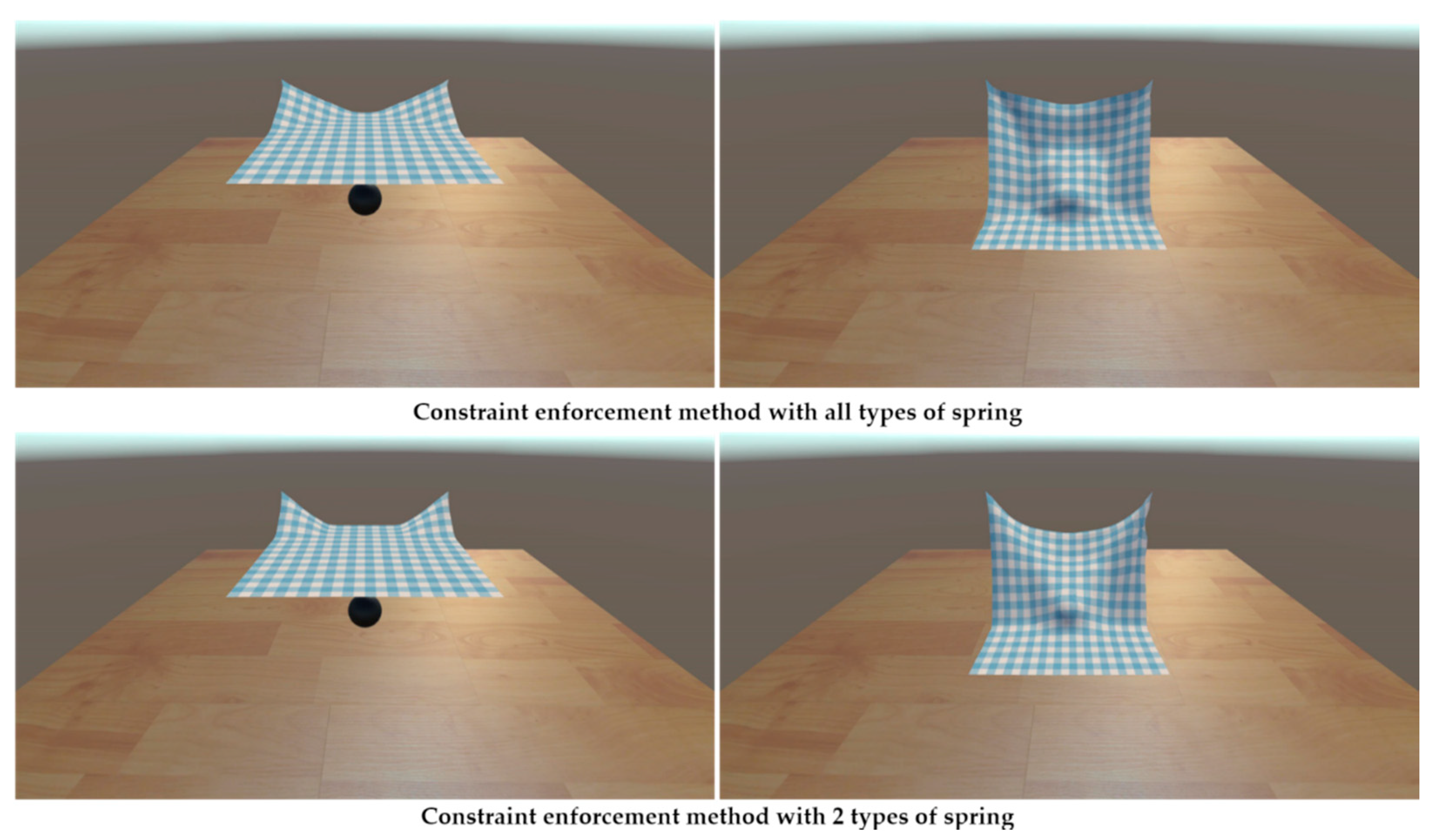
• Cloth simulation is implemented based on the mass–spring system, implicit constraint enforcement, and adaptive constraint activation and deactivation (ACAD), using Unity3D compute shader.
• The parallel method of a sparse linear solving algorithm is utilized to accelerate the performance of the constraint enforcement method.

The rest of the paper is organized as follows. Section 2 provides an overview of the previous studies of cloth simulation. Section 3 presents the proposed method for implementation based on the mass–spring system and constraint enforcement on GPU. Section 4 compares the performance result of the cloth simulation using the mass–spring system, constraint enforcement, and ACAD method that are implemented on Unity3D compute shader. To compare and contrast each method in an understandable manner, we conduct an experiment under the scenario in which a cloth object collides with a spherical object. Section 5 concludes the paper.

2. Related Work

Previous approaches that have focused on cloth simulation in real-time have been studied to represent relatively simple models, which concentrated on faster algorithms. The finite element method (FEM) has been proven to be an accurate approach to simulate deformable models [10]. FEM is a time-consuming method, due to the method of dividing an object into a large number of elements, and solving a large system of equations. However, many approaches have improved FEM techniques to be used in real-time simulation [11,12,13]. Mesh simplification approaches have been studied to simplify the detail of the 3D object and maintain the quality of the mesh [14].

Müller et al. [15] applied a position-based dynamic (PBD) method to simulate the deformable cloth object. The position-based method is fast, stable, and robust, but is not an accurate method. Hence, the velocity and force properties are ignored in PBD, which directly change the position of each node using project position to satisfy all constraints.

Many force-based methods have been researched and applied to the real-time simulation of deformable cloth objects. The explicit and implicit methods are used to obtaining a numerical approximation to the solution of time-dependent equations [16]. The explicit Euler method is a first-order method of linear approximation, which uses a discrete time-step to approximate the solution of the motion equation. Since the explicit method is relatively inaccurate compared to the implicit method, it requires less operation, and is simple to implement. The position and velocity of a node are affected by the internal force and external force, and the acceleration can be computed based on Newton’s second law of motion. The mass–spring system method of deformable cloth simulation was first introduced by Provot [17]. Georgii et al. [18] proposed a GPU structure to solve a numerical equation of the mass–spring method with an efficient memory access pattern using OpenGL architecture. Similarly, Mosegaard et al. [19] accelerated a spring-mass system for a surgical simulator that was implemented on the OpenGL platform.

In the mass–spring system method, a spring’s force is used to maintain the distance of the spring at each given time-step. However, the distance of each spring that can be stretched or compressed causes a numerical problem. Provot [17] applied a dynamic inverse constraint on springs that were over-elongated to prevent the “super-elastic” effect. As the result, this method could help a model perform realistically, but the displacement of each node directly ignored the physical consequence of the dynamic behavior of motion. Consequently, an implicit constraint was used to solve the elongated springs beyond 10%, and to prevent the excessive elongation of springs [20]. Goldenthal et al. used a smaller threshold of (1 and 0.1)% to simulate a piece of cloth that was quite stiff [21].

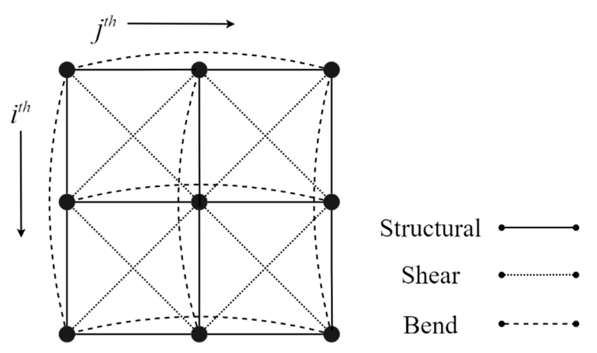
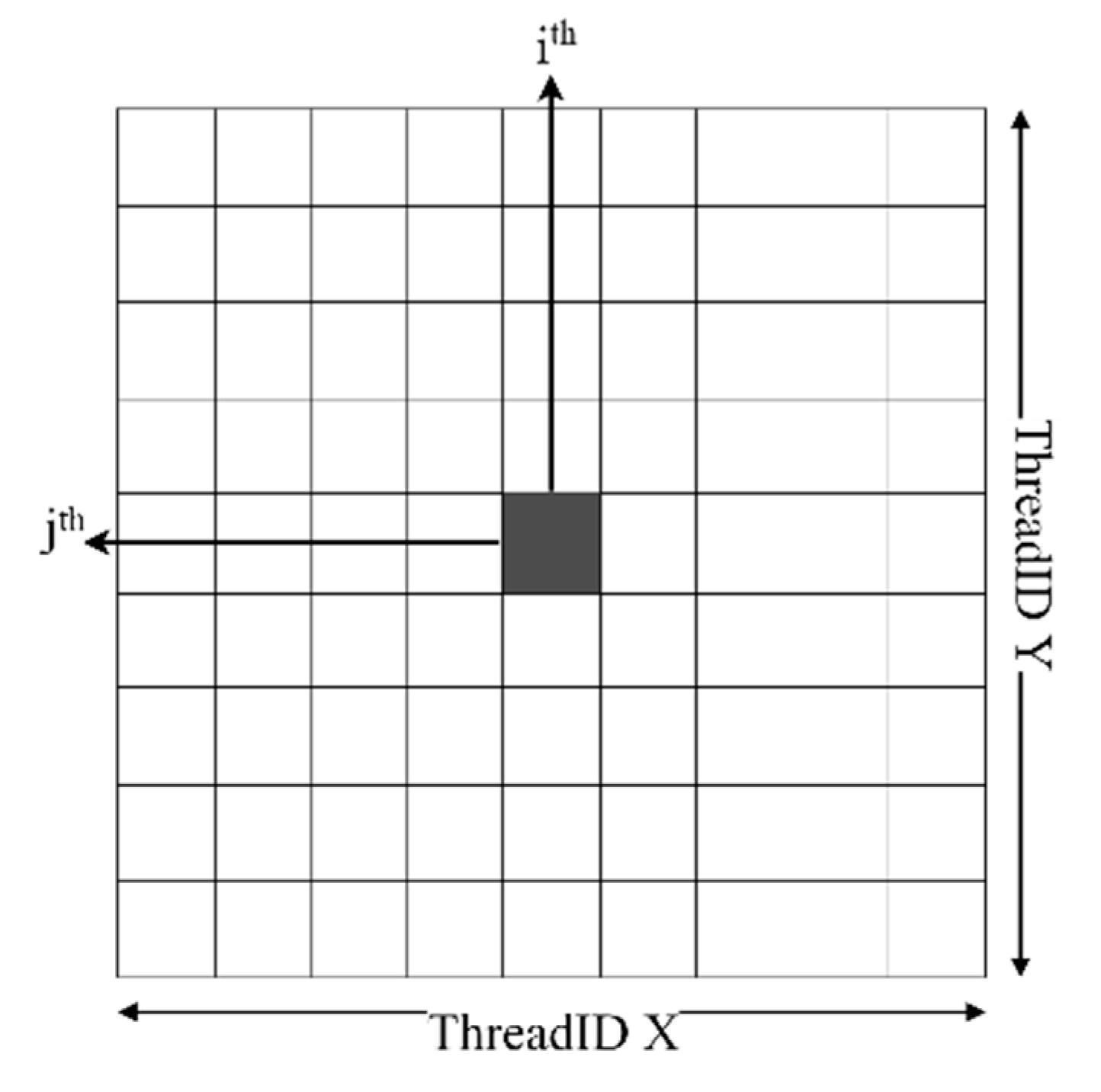
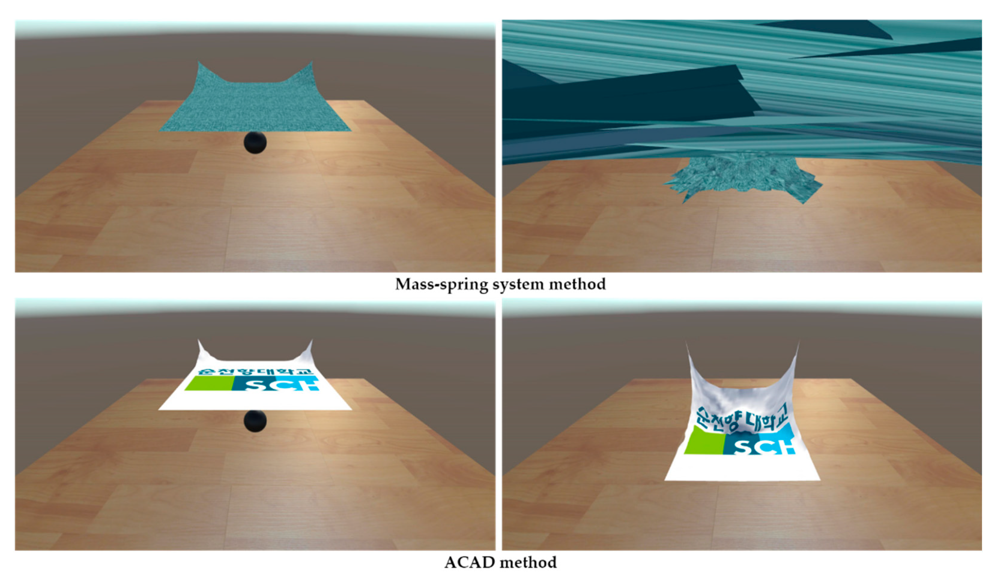
2.1. Mass–Spring System

The mass–spring damper model consists of a list of springs that are defined at the initializing stage of the simulation. Each spring is made by 2 nodes and denoted by p₁ and p₂ as the first and second node positions, respectively. Similarly, the velocities are denoted by v₁ and v₂, and the initial length or rest length of the spring is L₀ [22]. Figure 1 illustrates the structure of the mass–spring model used in the cloth simulation. A node can be linked with other nodes in the grid where i and j are the coordinates (row and column indices) of the 2D grid.

General nodes can have 12 links except corner nodes and side nodes that have a different number of links since their neighbor nodes do not exist. Therefore, three types of spring can be classified as follows:

• Structural springs: node [i, j] can be linked with node [i, j+1], [i, j-1], [i+1, j], [i-1, j].
• Shear springs: node [i, j] can be linked with node [i+1, j+1], [i+1, j-1], [i-1, j-1], [i-1, j+1].
• Bend springs: node [i, j] can be linked with to node [i, j+2], [i, j-2], [i+2, j], [i-2, j].

In the edge-centric algorithm, the spring force is computed using Hooke’s law. Variable K_s is added to the force equation to increase the stiffness of the spring, and parameter K_d is the damping coefficient of the spring. Note that the edge-centric algorithm obtains two different directions of forces to each node in the spring. The force equation of the edge-centric algorithm can be written as follows in Equations (1) and (2):

$$f_1=\left[k_s\left(\left|p_2-p_1\right|-L_0\right)+k_d\left(\frac{\left(v_2-v_1\right) · \left(p_2-p_1\right)}{\left|p_2-p_1\right|}\right)\right]\frac{p_2-p_1}{\left|p_2-p_1\right|}$$

(1)

$$f_2=-f_1$$

(2)

where, f₁ and f₂ are the forces of the first node and second node in a spring. After spring force computation, the accumulation of the force on each node is computed separately. Differently, in the node-centric algorithm, each node accumulates the force from all springs directly at the same time.

2.2. Implicit Constraint Enforcement

In research by Hong et al. [23], the implicit constraint enforcement method predicts the correct direction of the constraint forces by using future time-step. A list of positions of 3n size is used, where q = [x₁, y₁, z₁, x₂, y₂, z₂… x_n, y_n, z_n]^T, and where n is the total number of all nodes. The distance constraint Φ based on Euclidean equation can be defined as follows:

$$\mathsf{\Phi }={\left(x_1-x_2\right)}^2+{\left(y_1-y_2\right)}^2+{\left(z_1-z_2\right)}^2-r^2$$

(3)

where, r is the initialing distance between 2 nodes. Then the list of m distance constraints can be written as the following equation:

$$\mathsf{\Phi }\left(q,t\right)={\left[{\mathsf{\Phi }}^1\left(q,t\right),{\mathsf{\Phi }}^2\left(q,t\right),\dots {\mathsf{\Phi }}^{\mathrm{m}}\left(q,t\right)\right]}^T$$

(4)

The partial differentiation on distance constraint concerning subscript q obtains a Jacobian matrix Φ_q of size of m × 3n. This can be calculated using the following equation:

$${\mathsf{\Phi }}_q\left(q,t\right)=\left[\begin{array}{ccccc}A& B& 0& \cdots & 0\\ 0& C& D& \cdots & 0\\ ⋮& ⋮& ⋮& \ddots & ⋮\end{array}\right]$$

$$\begin{gathered} A=\left|2\left(x_0-C_x\right),2\left(y_0-C_y\right),2\left(z_0-C_z\right)\right|, \\ B=\left|-2\left(x_0-C_x\right),-2\left(y_0-C_y\right),-2\left(z_0-C_z\right)\right|, \\ C=\left|2\left(x_1-C_x\right),2\left(y_2-C_y\right),2\left(z_2-C_z\right)\right|, \\ D=\left|-2\left(x_1-C_x\right),-2\left(y_1-C_y\right),-2\left(z_1-C_z\right)\right|, \end{gathered}$$

(5)

where, x₀, y₀, z₀ are the current position of a node, and C_x, C_y, C_z are the fixed position of the node. The system of constraint force equation can be written as follows:

$$M\ddot{q}+{\mathsf{\Phi }}_q^T\lambda =F^A$$

(6)

where, M is the mass matrix and the diagonal element stores the node’s mass, F^A is the accumulation of gravity force and constraint forces acting on the node, ${\Phi }_q^T$ is the transpose of the Jacobian matrix, and λ is the Lagrange multiplier vector of size m. The equation of time integration can be defined as follows in the equation:

$$\dot{q}\left(t+\mathsf{\Delta }t\right)=\dot{q}\left(t\right)-\mathsf{\Delta }t{M}^{-1}{\mathsf{\Phi }}_q^T\lambda +\mathsf{\Delta }t{M}^{-1}{F}^A\left(q,t\right)$$

(7)

$$q\left(t+\mathsf{\Delta }t\right)=q\left(t\right)+\mathsf{\Delta }t\dot{q}\left(t+\mathsf{\Delta }t\right)$$

(8)

The integration time-step is Δt, so the constraint function of the next time is treated implicitly, as follows in Equation (9):

$$\mathsf{\Phi }\left(q\left(t+\mathsf{\Delta }t\right),t+\mathsf{\Delta }t\right)=0$$

(9)

A truncated, first-order Taylor series can be used to estimate Equation (9), and the new constraint function of next time can be written as follows:

$$\mathsf{\Phi }\left(q\left(t\right),t\right)+{\mathsf{\Phi }}_q\left(q\left(t\right),t\right)\left(q\left(t+\mathsf{\Delta }t\right)-q\left(t\right)\right)+{\mathsf{\Phi }}_t\left(q\left(t\right),t\right)\mathsf{\Delta }t=0$$

(10)

To eliminate q(t + Δt), Equations (7) and (8) are substituted into Equation (9). Putting all of this together, we can solve the Lagrange multiplier by solving a system of linear equations, as follows in Equation (11):

$${\mathsf{\Phi }}_q\left(q,t\right)M^{-1}{\mathsf{\Phi }}_q^T\lambda =\frac{1}{\mathsf{\Delta }{t}^2}\mathsf{\Phi }\left(q,t\right)+\frac{1}{\mathsf{\Delta }t} {\mathsf{\Phi }}_t\left(q,t\right)+{\mathsf{\Phi }}_q\left(q,t\right)\left(\frac{1}{\mathsf{\Delta }t}\dot{q}\left(t\right)+M^{-1}{F}^A\left(q,t\right)\right)$$

(11)

Equation (11) is in the form of a linear system problem, and can be solved by a precise and effective method. The conjugate gradient is the most well-suited algorithm for this kind of system [24]. Equation (11) can be written as Aλ = B. The conjugate gradient method is given by the following equation. The prediction vector, λ initializes with 0. Equation (12) can written as r₀ = p₀ = B. The routine to correct a prediction vector with i number of iterations can be written as follows:

$$r_0=p_0=B-A\lambda$$

(12)

$${\alpha }_i=\frac{r_i^T{r}_i}{p_i^{T}A{p}_i}$$

(13)

$${\lambda }_{i+1}={\lambda }_i+{\alpha }_i{p}_i$$

(14)

$$r_{i+1}=r_i-{\alpha }_{i}A{p}_i$$

(15)

$${\beta }_i=\frac{r_{i+1}^T{r}_{i+1}}{r_i^T{r}_i}$$

(16)

$$p_{i+1}=r_{i+1}+{\beta }_i{p}_i$$

(17)

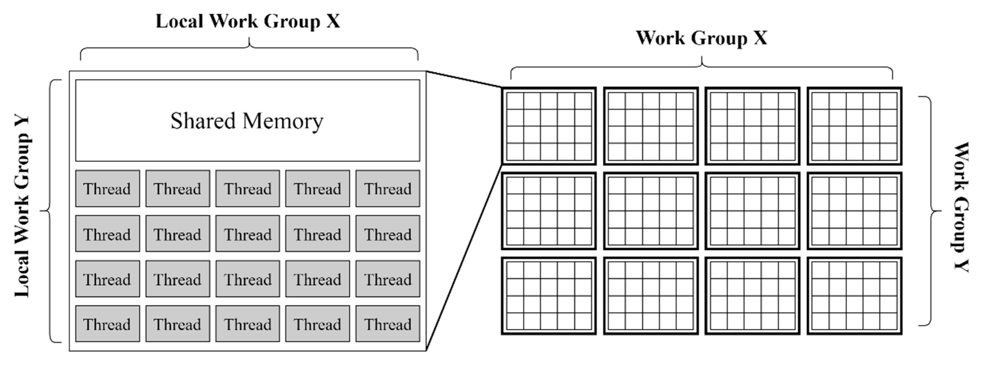
2.3. Unity3D Compute Shader

In general, a Unity engine offers primary scripting written in C# programming language to manage the general computation of object movement in the physics simulation [25]. Since the general C# script executes all operations as a serial process, there are limitations on the performance. Under these circumstances, the task of parallelism can provide a better performance, since all operations are executed in the background on their own thread. However, data parallelism in the GPU (also known as single instruction multiple data) achieves a promising performance for the general purpose of physically based simulation, since the computation and rendering have been done in the GPU.

Therefore, Unity3D provides the solution for GPU utilization by using Microsoft’s DirectCompute 5.0 technology. Compute Shaders in the Unity engine is key to performing general-purpose computing on the GPU. The compute shader is a programmable shader stage that extends Microsoft Direct3D 11′s capabilities beyond graphics programming. Like other shaders (vertex and fragment shader), a compute shader follows the syntax of high-level shader language (HLSL). Normally, the compute shader script in Unity3D is written in HLSL, and compiled to a specific platform (DirectX or OpenGL core). Therefore, the hierarchy of the compute shader in Unity3D is similar to the compute shader in OpenGL, but the compute shader in Unity3D consists of multiple kernels, unlike in OpenGL, which consists of a single kernel per compute shader. The compute space is required to manage the number of threads in the local group. Additionally, the compute space of the kernel is dependent on the algorithm and the problem of data. Figure 2 illustrates the scheme of the compute space of the kernel.

Compute space can be defined either as 1D, 2D, or 3D of the workgroup using Unity’s API in dispatching the function of compute shader, where each workgroup consists of a local workgroup with shared memory that can be used for any thread in the same local workgroup. The dimension of each local workgroup can be defined either as 1D, 2D, or 3D of the thread, and is specified in the kernel of compute shader [26]. Note that each thread in the local workgroup is executed in a non-sequential order, which gives an advantage to the performance of the extremely large data. On the other hand, the data to be used in the kernel must be ComputeBuffer type, which contains large arrays of structured data. It can share with different kernels in a compute shader or the other compute shader as well.

3. Implementation of Cloth Simulation in Unity3D

In this section, we provide several techniques for the implementation of a cloth simulation system in GPU. First, we describe the implementation method of MSS using compute shader in Unity3D. We then describe the method to simulate the cloth model using constraint enforcement. Significant information of the simulation includes the node’s position, velocity, force, and normal vector, which are stored in ComputeBuffer object. We use a simple sheet model to represent the cloth object.

3.1. Mass–Spring System on the GPU

In Figure 1, there are 12 directions of force acting on a single node. So, we use a node-centric algorithm to accumulate the force of each node using the 1 thread per node technique. Since the node in a cloth model can be represented as 2D, we can define the compute space using the 2D dimension of the workgroup that each local workgroup determined as (x = 32, y = 32, z = 1) in the kernel. Consequently, the dimension of the workgroup is calculated as (x = $\lceil \frac{\mathrm{Row}}{32}\rceil$, y = $\lceil \frac{\mathrm{Column}}{32}\rceil$, z = 1), where Row and Column are the numbers of nodes in the row and column of a cloth model, respectively.

To invoke each element of the buffer by the index of buffer properly, the index of the 2D thread is calculated following the scheme demonstrated in Figure 3. ThreadID is used to indicate a thread throughout the entire distribution in the thread group in the form of 3D format, and can be calculated by GroupID × ThreadGroupSize + GroupThreadID, where GroupID refers to the index of a specific workgroup, ThreadGroupSize is the total number of how many workgroups there are in the compute space, and GroupThreadID is a unique index of the thread in each local workgroup (local index).

We then calculate the index of the buffer as 1D by jth × Column + ith, where ith and jth are the indices of the thread in the X and Y-axis of ThreadID, respectively. Algorithm 1 indicates the pseudo-code of the kernel to accumulate the spring force. Note that the ComputeSpringForce() function follows Equation (1), which requires the position and velocity of 2 nodes to manipulate the force as a result.

Algorithm 1 The node’s centric algorithm to accumulate spring force.

Spring force accumulation kernel

Input: Buffer Position, Velocity, Force            Output: Buffer Force Begin   i ← ThreadID.x   j ← ThreadID.y   index ← j×column+i   Force[index] ← ComputeSpringForce(node[i, j], node[i, j+1])   Force[index] ← ComputeSpringForce(node[i, j], node[i, j-1])   Force[index] ← ComputeSpringForce(node[i, j], node[i+1, j])   Force[index] ← ComputeSpringForce(node[i, j], node[i-1, j])   Force[index] ← ComputeSpringForce(node[i, j], node[i+1, j+1])   Force[index] ← ComputeSpringForce(node[i, j], node[i+1, j-1])   Force[index] ← ComputeSpringForce(node[i, j], node[i-1, j-1])   Force[index] ← ComputeSpringForce(node[i, j], node[i-1, j+1])   Force[index] ← ComputeSpringForce(node[i, j], node[i, j+2])   Force[index] ← ComputeSpringForce(node[i, j], node[i, j-2])   Force[index] ← ComputeSpringForce(node[i, j], node[i+2, j])   Force[index] ← ComputeSpringForce(node[i, j], node[i-2, j]) End

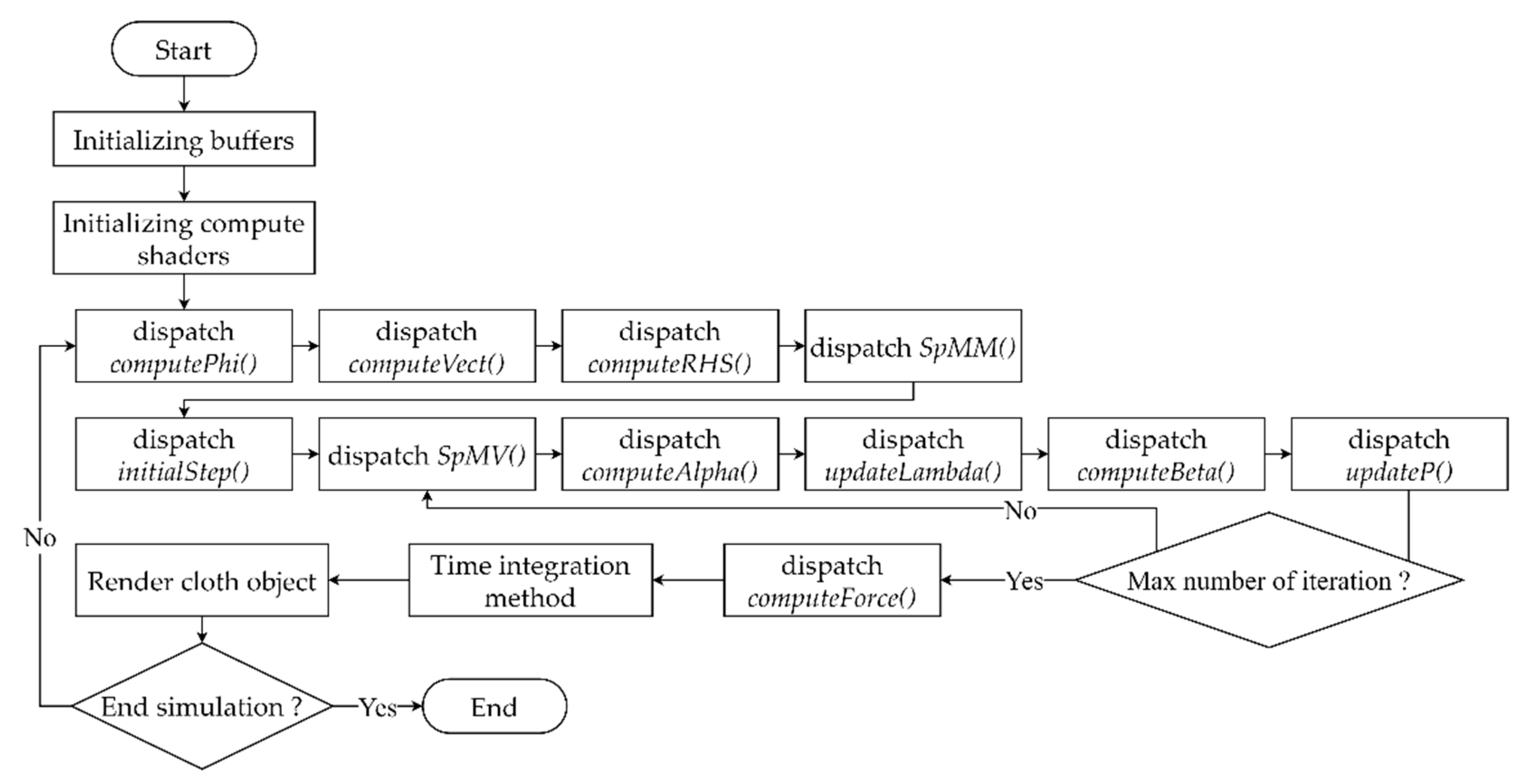
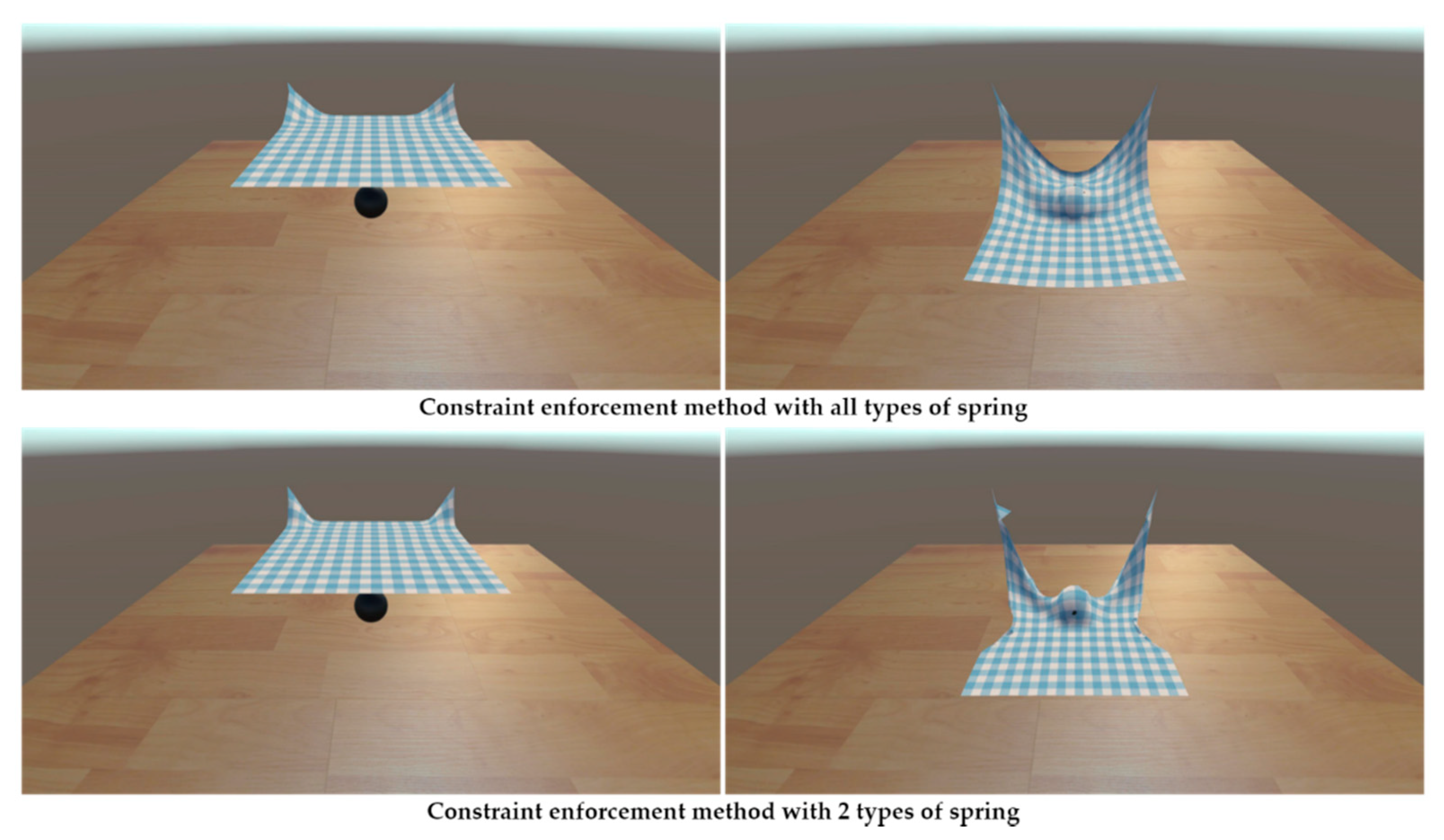
3.2. Constraint Enforcement on the GPU

From Equation (11), we classify the operation into three parts, constructing a sparse linear system, solving a sparse linear system, and computing constraint force. So, we use three different compute shaders, and each computes shader consists of multiple kernels, as shown in

Table 1. List of compute shaders to use in the constraint enforcement algorithm.

Compute Shader	Kernel	Number of Workgroups	Thread in a Local Workgroup
ConstructingSys	computePhi()	$( \lceil \frac{\mathrm{Constraints}}{1024}\rceil ,1,1)$	(1024, 1, 1)
	computeVect()	$( \lceil \frac{\mathrm{Nodes}}{1024}\rceil ,1,1)$	(1024, 1, 1)
	computeRHS()	$( \lceil \frac{\mathrm{Constraints}}{1024}\rceil ,1,1)$	(1024, 1, 1)
	SpMM()	$( \lceil \frac{\mathrm{Constraints}}{32}\rceil ,\lceil \frac{\mathrm{Constraints}}{32}\rceil ,1)$	(32, 32, 1)
LinearSystemSolving (Conjugate Gradient)	initialStep()	$( \lceil \frac{\mathrm{Constraints}}{1024}\rceil ,1,1)$	(1024, 1, 1)
	SpMV()	$( \lceil \frac{\max \left(\mathrm{nnz}\right)}{1024}\rceil ,1,1)$	(1024, 1, 1)
	computeAlpha()	$( \lceil \frac{\mathrm{Constraints}}{1024}\rceil ,1,1)$	(1024, 1, 1)
	updateLambda()	$( \lceil \frac{\mathrm{Constraints}}{1024}\rceil ,1,1)$	(1024, 1, 1)
	computeBeta()	$( \lceil \frac{\mathrm{Constraints}}{1024}\rceil ,1,1)$	(1024, 1, 1)
	updateP()	$( \lceil \frac{\mathrm{Constraints}}{1024}\rceil ,1,1)$	(1024, 1, 1)
ConstraintForce	computeForce()	$( \lceil \frac{\mathrm{Constraints}}{1024}\rceil ,1,1)$	(1024, 1, 1)

:

A Jacobian matrix (J) is obtained by partial differentiation of the distance constraint equation and consists of lots of zero values. In this case, the sparse matrix format is the most suitable in terms of memory allocation and performance, since it contains only non-zero (nnz) values. The J matrix has m × 3n size, and each row possibility consists of 6 nnz values. As a result, the nnz elements are arranged uniformly near the diagonal of a matrix J. General operation, such as sparse matrix–matrix multiplication (SpMM), sparse matrix–vector multiplication (SpMV), and transpose sparse matrix–vector multiplication (SpMVT), is the bottleneck in the simulation.

Under these circumstances, ELLPACK and Compressed Sparse Row (CSR) format are considered for the structure of the J matrix. ELLPACK format obtains a good result of the performance as compared to CSR format, but CSR format has an advantage over ELLPACK in being faster at performing the SpMVT operation [27]. In CSR format, there are three lists to represent the non-zero values, a list of the non-zero elements (A), a list of the column indices of the non-zero elements (JA), and a list of the compressed row indices of the non-zero elements (IA). Note that the list of the compressed row indices is of length m + 1, and each element of the IA points to row starts in the JA and A.

Another advantage of the CSR format is a self-transpose operation, which does not require an additional operation to transpose each element of the J matrix. From the idea of CSR format, the new transpose of J matrix can now be stored in Compress Sparse Column (CSC) that has three lists similar to the CSR format. The transpose of CSR format, denoted by B, obtains the same order of the three lists, the IB list now represents the row indices of the non-zero elements, and the JB list is a list of the compressed column indices of the non-zero elements.

The size of the system matrix in Equation (11) is m × m, but it is a sparse matrix, so it can be represented by coordinate sparse matrix format (COO), and it stores each non-zero element in a list of triplets (nnz value, row index of the non-zero value, column index of the non-zero value).

Table 2. List of the buffers used in constraint enforcement algorithm.

Buffer	Size	Data Type	Description
Phi	m	Float	Vector Φ(q, t)
Vect	3n	Float	$\mathrm{Vector} \left(\frac{1}{\mathsf{\Delta }t}\dot{q}\left(t\right)+M^{-1}{F}^A\left(q,t\right)\right)$.
Rhs	m	Float	Right-hand side vector of Equation (11)
Lambda	m	Float	a vector Lagrange Multiplier (λ)
A	6 × m	Float	Vector of nnz value
IA	m + 1	Integer	Compressed row index for nnz value of A
JA	6 × m	Integer	Column Vector of A indices
IB	6 × m	Integer	Row Vector of B indices
JB	m + 1	Integer	Compressed column index for nnz value
Sys	nnz	Vector3	System matrix of Equation (11)
nnz	1	Integer	Number of the non-zero value of the system matrix
Force	3n	Float	Vector of constraint force

shows the list of buffer objects used in constraint enforcement. Since the size of the buffer to store data is static and cannot be changed during the simulation process, each buffer is initialized with a defined number.

In order to perform cloth simulation using constraint enforcement method using the kernel in GPU, a ComputeShader.Dispatch() function is called in a simulation loop with the given kernel name and specific size of the workgroup. Note that each kernel in a compute shader performs a specific task and each kernel is performed after the process of the previous kernel is finished. So, between calling each kernel, a synchronization is performed in the abstract, to avoid the issue of the process interruption and thread divergence. Due to the different dimensions of data, the linear solving algorithm is divided into multiple kernels with a different number of threads. Figure 4 demonstrates a flowchart of the proposed algorithm to compute constraint force using kernels in compute shader.

As shown in the flowchart, at the start of simulation all GPU buffers are initialized and data are filled in the array of the buffer. In the initializing stage of compute shader, the specific buffer is required to allow permission of the buffer manipulation in the GPU kernel, and a uniform variable can also be put in at this stage. Henceforth, the simulation loop is performed by dispatching computePhi() kernel to compute the ${\mathsf{\Phi }}_t\left(q,t\right)$, a vector in GPU, and stores in the Phi buffer. In the same kernel, the Jacobian matrix (Φ_q) is created as well. After that, the simulation dispatches computeVect() kernel to compute the $\left(\frac{1}{\mathsf{\Delta }t}\dot{q}\left(t\right)+M^{-1}{F}^A\left(q,t\right)\right)$ vector, and stores in Vect buffer. The right-hand side of the system is then computed by dispatching computeRHS(), and the result of ( $\frac{1}{\mathsf{\Delta }{t}^2}\mathsf{\Phi }\left(q,t\right)+\frac{1}{\mathsf{\Delta }t} {\mathsf{\Phi }}_t\left(q,t\right)+{\mathsf{\Phi }}_q\left(q,t\right)\left(\frac{1}{\mathsf{\Delta }t}\dot{q}\left(t\right)+M^{-1}{F}^A\left(q,t\right)\right))$ is stored in Rhs buffer. In consequence, the system matrix that is stored in the COO can be computed by the SpMM kernel as expressed in Algorithm 2:

Algorithm 2 The SpMM algorithm kernel.

SpMM

Input: Buffer A, IA, JA, IB, JB        Output: Buffer Sys Begin   i ← ThreadID.x   j ← ThreadID.y   rowStart ← IA[i]   rowEnd ← IA[i+1]   colStart ← JB[j]   colEnd←JB[j+1]   value ← 0   for ia ← rowStart to rowEnd do:     colIndex ← JA[ia]     for jb ← colStart to colEnd do:       rowIndex ← IB[jb]       if colIndex == rowIndex do:         value ← value + (A[ia] × A[jb])       end if     end for   end for   if value != 0 do:     InterlockAdd(nnzIndex,1)     COO[nnzIndex] ← float3(i,j,value)   end if End

An atomic operation is required to increase the index of the COO matrix and to avoid data racing when writing a new value to the nnz buffer. The next step is a linear solving process that applies a conjugate gradient (CG) algorithm and implements it on multiple kernels. The most significant operation of the CG algorithm is the SpMV operation, COO matrix multiply with vector. Algorithm 3 shows the pseudocode of the SpMV kernel:

Algorithm 3 The SpMV algorithm kernel.

SpMV

Input: Buffer Sys, nnz, P        Output: Buffer Result Begin   i ← ThreadID.x   if i < nnz do:     nnz_row ← Sys[i].x     nnz_col ← Sys[i].y     nnz_value ← Sys[i].z     result ← nnz_value × P[nnz_col]     InterlockAddFloat(Result[nnz_row],result)   end if End

In the SpMV kernel, the function InterlockAdd() is not supported with floating-point value, so an InterlockedCompareExchange() is used instead to perform concurrent sum on the element buffer with the uint data type, and the new uint data type is then converted to float data type. The simulation dispatches all kernels in the CG compute shader to obtain the approximated value buffer; the lambda buffer is then used to compute constraint force based on Equation (6), and applies the SpMVT algorithm. The algorithm of SpMVT is inspired by the research of Steinberger et al. [28], to compute the constraint force, and uses the node’s force in time integration method to find the next position of the nodes in a cloth object. The position of all nodes is used to rendering the cloth object as well.

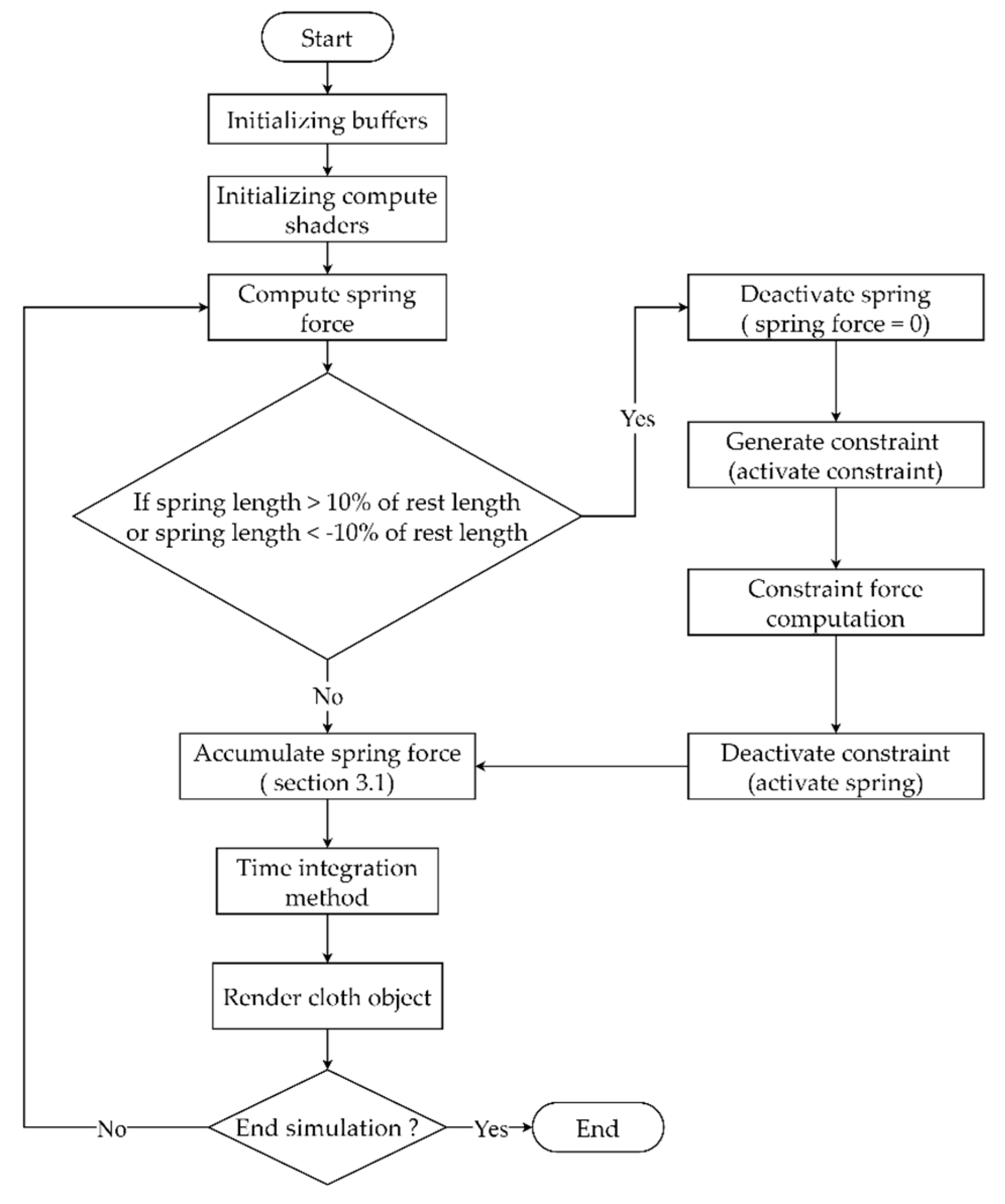
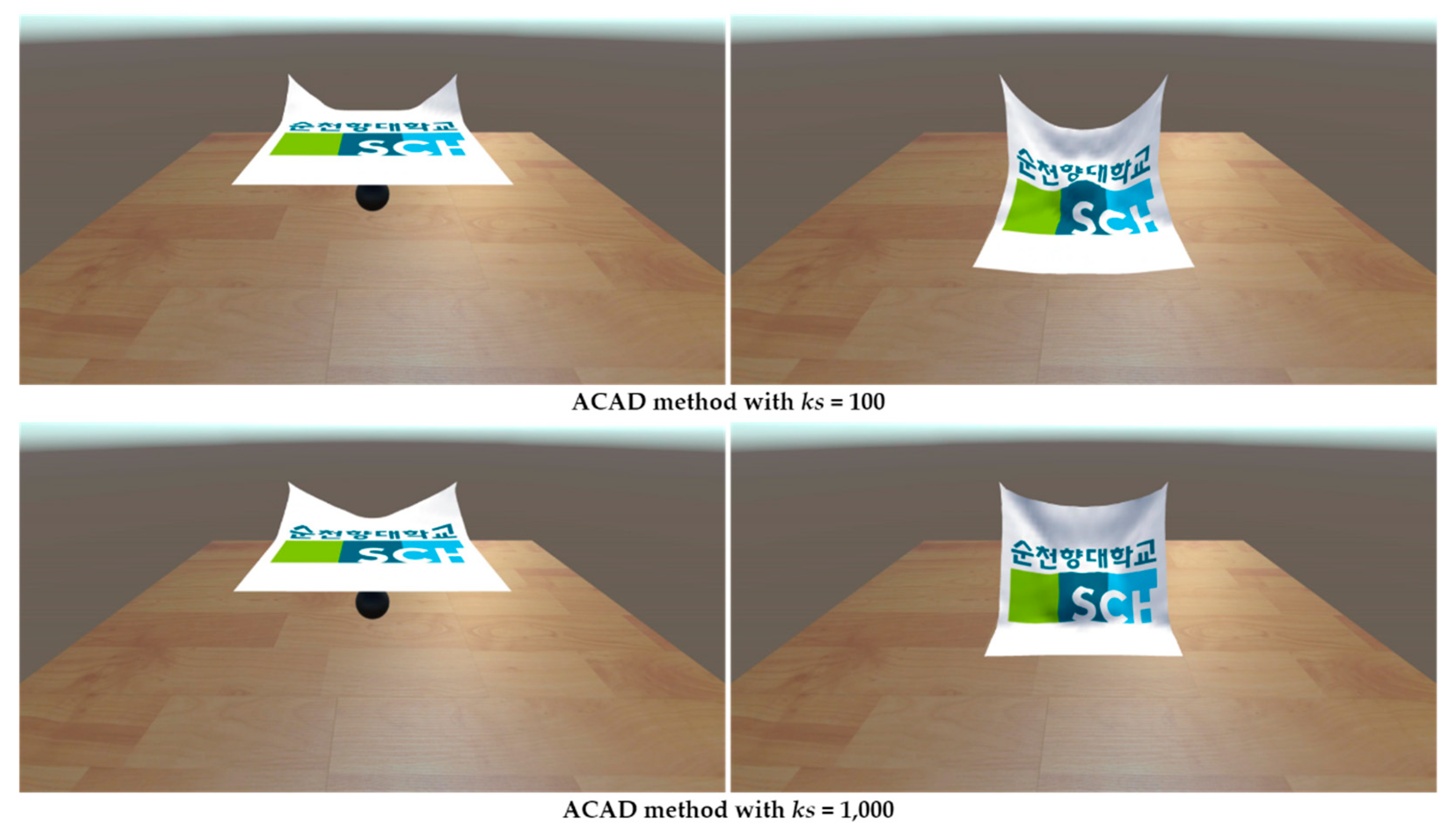
3.3. Adaptive Constraint Activation and Deactivation

The constraint enforcement attempts to solve a large data in each frame of the simulation. Therefore, the ACAD method is properly used. Figure 5 demonstrates a flowchart of the ACAD method. Both the mass–spring system and constraint enforcement are used in the ACAD method to reduce the computational burden of constraint enforcement.

In the mass–spring system, a spring can be compressed or stretched in each frame of the simulation, and accurate force is used to prevent the elongation of spring. The process of the ACAD starts from the computation of spring force; at the same time the current length or spring is computed, and compared to a defined threshold. If the spring exceeds 10% of the spring rest length, those springs are deactivated, and generate the implicit constraint or activate constraint in order to find the constraint force. The implicit constraint can be deactivated after the constraint force is found using the constraint enforcement method. As a result, the spring force and constraint force are accumulated together for each node to perform the time–integration method, and displace the node’s position.

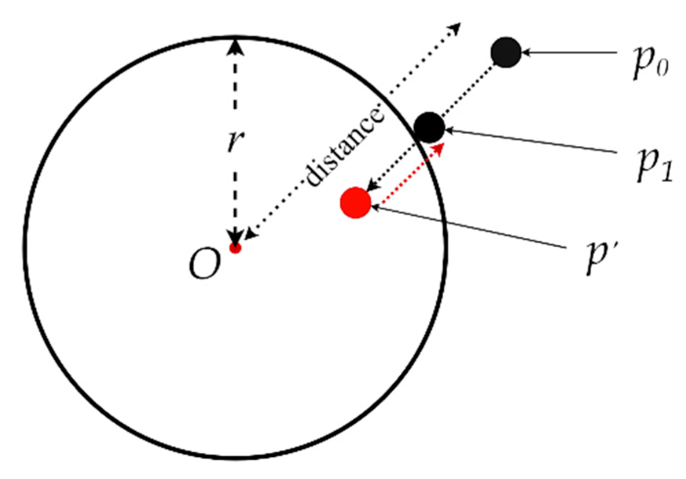
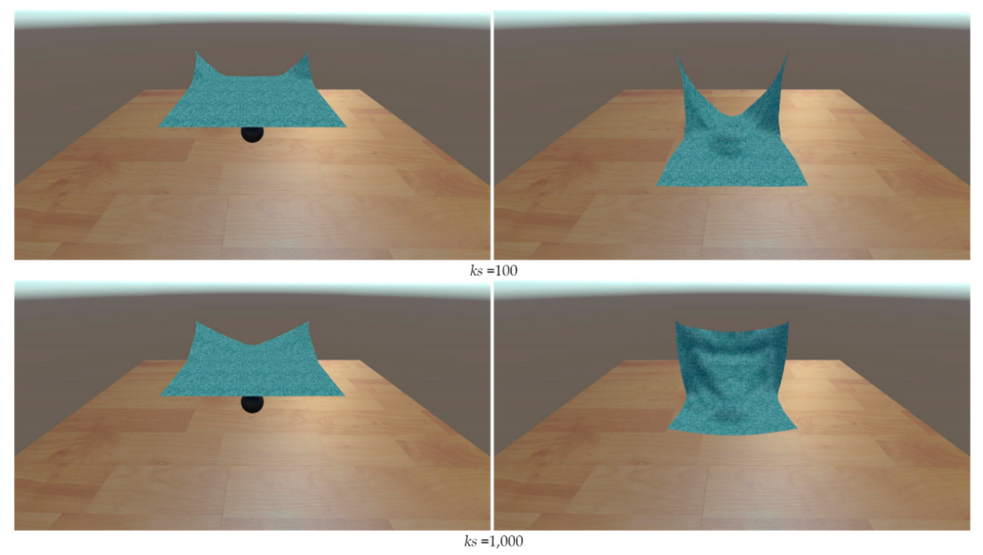
3.4. Cloth–Sphere Collision Detection and Response

In this section, we describe how the cloth object performs collision detection and the response algorithm with the 3D sphere object. In Unity3D, there is a 3D sphere object with a sphere collider, so we use node–sphere distance in order to detect the collision at each frame after the time–integration method is performed. Figure 6 illustrates the scenario when a node in the cloth model collides and before it collides with a spherical object.

In Figure 6, the old position is by p₀ and the new position is p₁. Let p^′ be the approximation of the new position after the p₀ is updated. Then, the distance between p^′ and the center O of a sphere can be calculated, and readily compared with the radius r of the spherical object. When the collision occurs, the distance between p^′ and the center O is smaller than the sphere’s radius r. The new position and velocity should be calculated according to solving this collision. Algorithm 4 demonstrates the proposed simple collision detection and response algorithm for the cloth simulation.

Algorithm 4 The algorithm for collision detection and response.

Collision detection and response

Input: p0, p′, v0, O, r, offset           Output: p1, v1 Begin   If distance(p′-O) < r do:     distance ← p0-O     p1 ← O + normalize(distance) × (r + offset)     v1 ← normalize(distance) + normalize(v0)   End if End

3.5. Normal Vectors Computation Based on Triangle Model on the GPU

Another property of the node, the normal vector is significantly used for rendering cloth objects with lighting and shadow casting. In a triangle of the cloth model, there are 3 vertices V₁, V₂ and V₃. To find a normal vector, the cross product of V₁₂ × V₂₃ is calculated, where V₁₂ = V₂ − V₁ and V₂₃ = V₃ − V₂. However, in the cloth model, all triangles are connected sequentially, then all normal vectors of the triangle are calculated, and the normal vectors of vertices are simultaneously accumulated. From the hierarchy to compute the spring force in the mass–spring system method, the same structure can be defined to compute each normal vector of a vertex concurrently. In a cloth mesh, a single vertex is connected with 8 triangles, which means that each thread performs the computation of the normal vectors, and accumulates the normal value from 8 triangles in 4 quadrants. Algorithm 5 shows the pseudo-code of the normal vector computation.

Algorithm 5 Pseudocode of the normal vector computation algorithm.

Normal vector computation

Input: Buffer Position           Output: Buffer Normal Begin   i ← ThreadID.x   j ← ThreadID.y   index ← j×column+i   n ← vector3(0,0,0)   n1 ← Compute n2 normal of 1st quadrant   n3 ← Compute normal of 2nd quadrant   n4 ← Compute normal of 3rd quadrant   n5 ← Compute normal of 4th quadrant   n ← ${\Sigma }_{i=1}^4{n}_i$   Normal [index] ← Normalize (n) End

4. Result

4.1. Experimental Environment

Table 3. Experimental environment.

Component	Specification
OS	Windows 10 Pro 10.0.1.19042 Build 19042
CPU	Intel® Core™ i7-7700
RAM	16 GB
GPU	NVIDIA GeForce GTX 1070 8 GB V-RAM
IDE	Unity 2020.3.8f1, Microsoft Visual Studio Community 2019 version 16.10.3
HLSL	Shader model 5.0
MAX thread per local workgroup	1024

shows the specifications with which our experiment was conducted on the desktop:

4.2. Rendering Method

We applied two different methods to render the proposed GPU cloth model using Unity3D. In the first method, the calculation has been done by compute shader that is dispatched in the C# script, and the vertices’ position are stored in the GPU buffer as well. The custom shader is required to shade the cloth object based on the vertices’ position and normal vector, then the ambient, diffuse, and specular lighting can be applied as well to render the cloth model. In the second method, a custom shader for shading the cloth object is optional, since it can use the default material that Unity provides to the mesh object. However, the disadvantage of this method is that it directly modifies the mesh’s vertices in the CPU. In consequence, it can cause further problems in terms of performance since the data transferring processing from GPU to CPU is time-consuming.

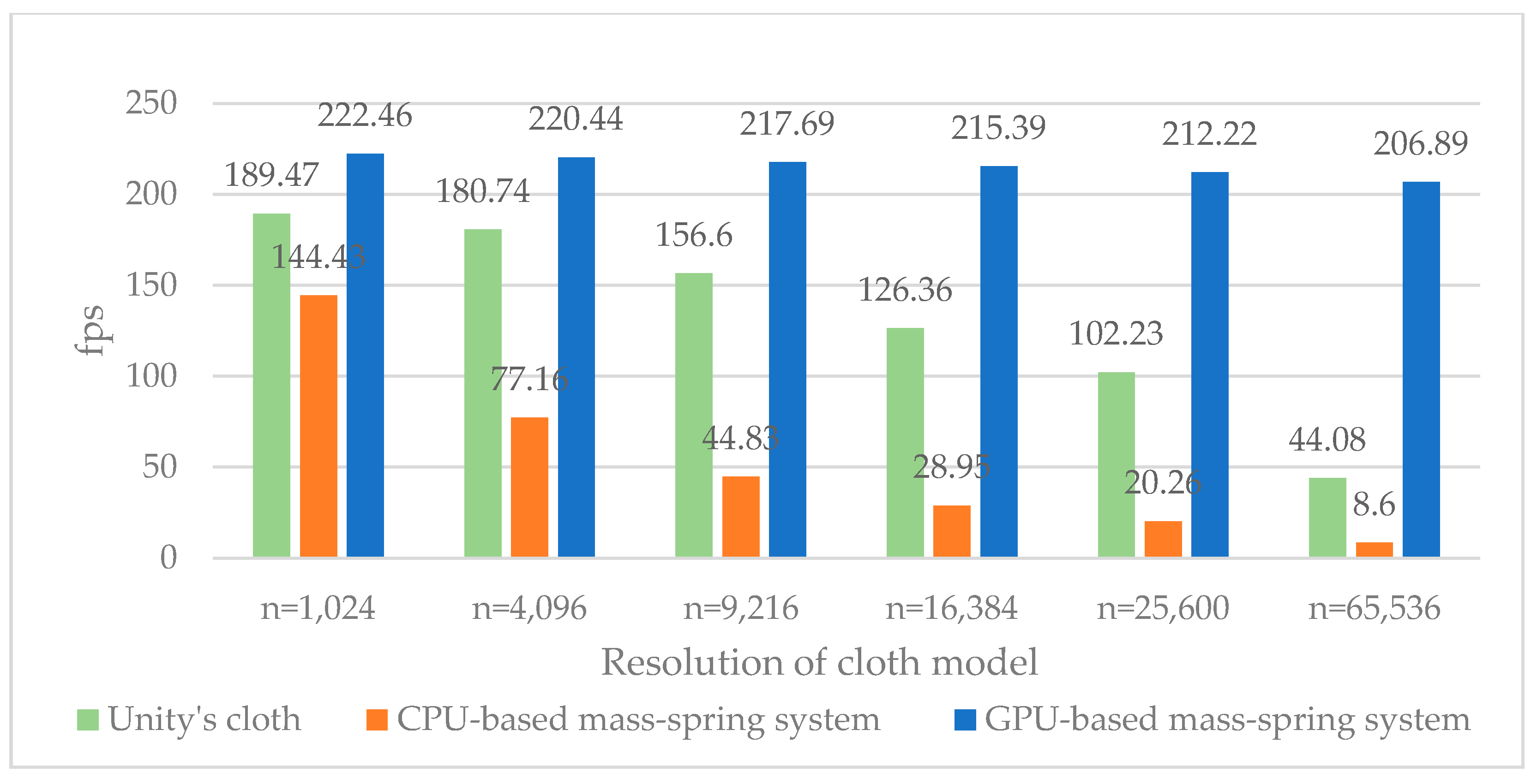
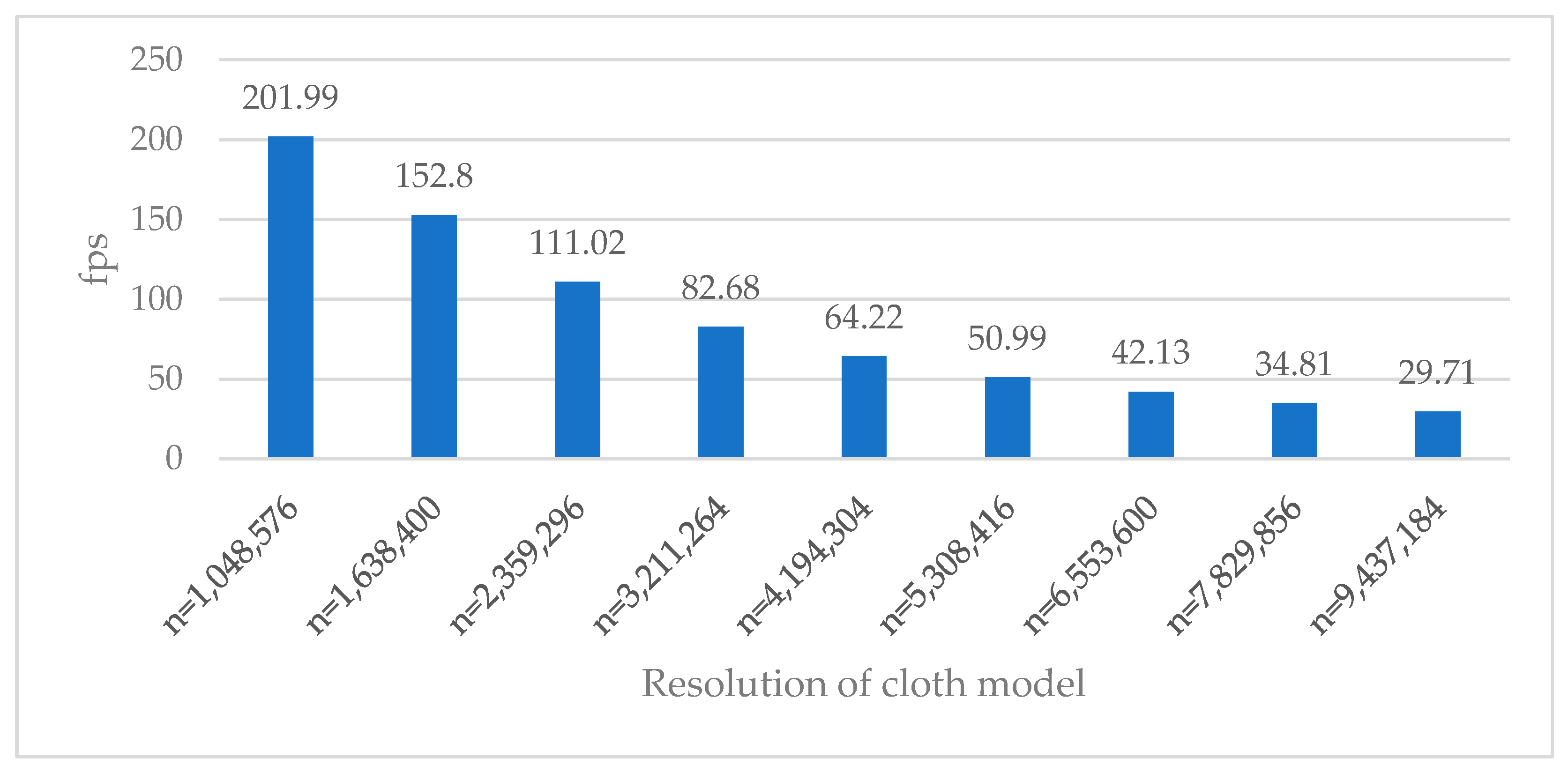
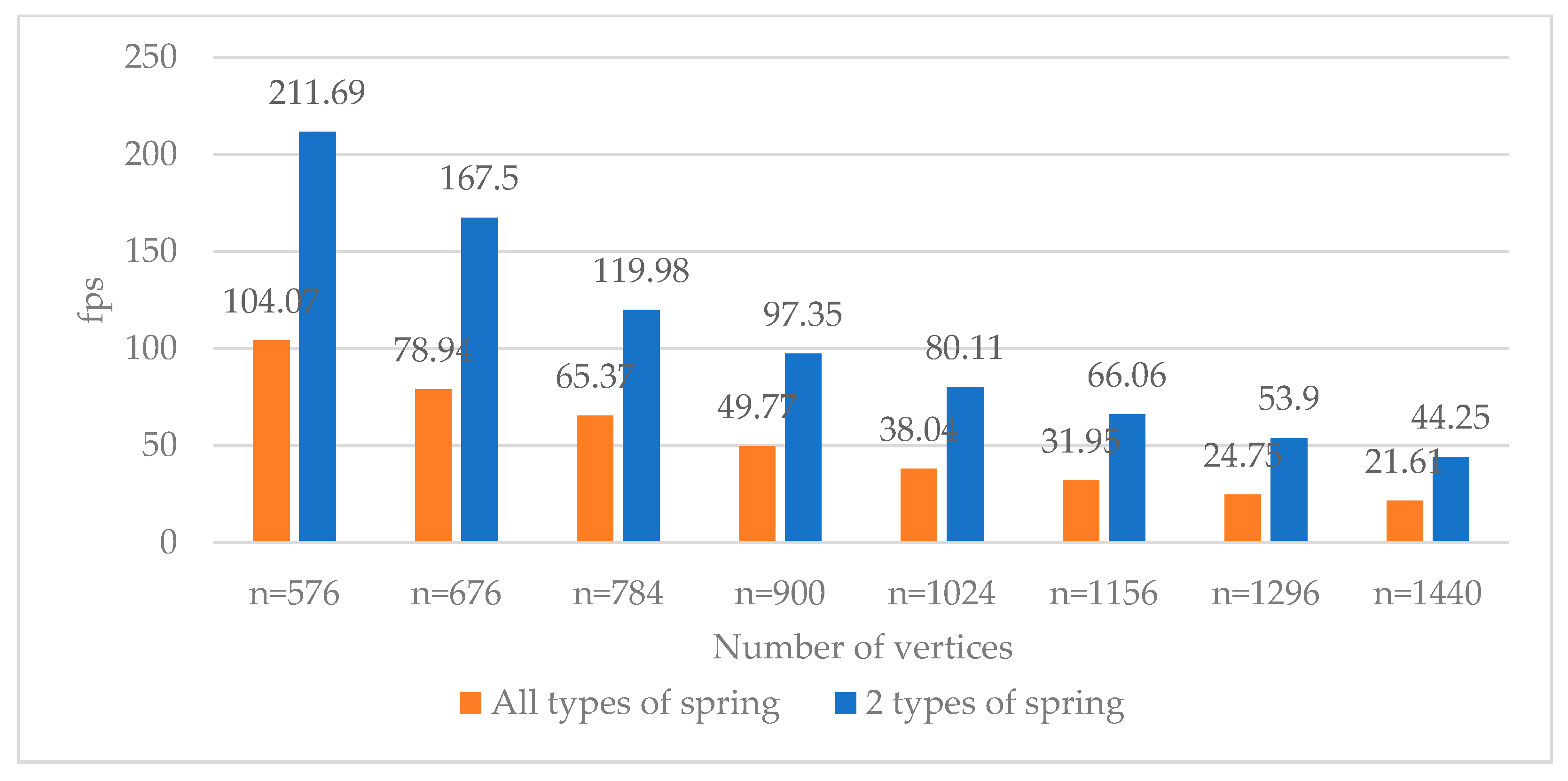
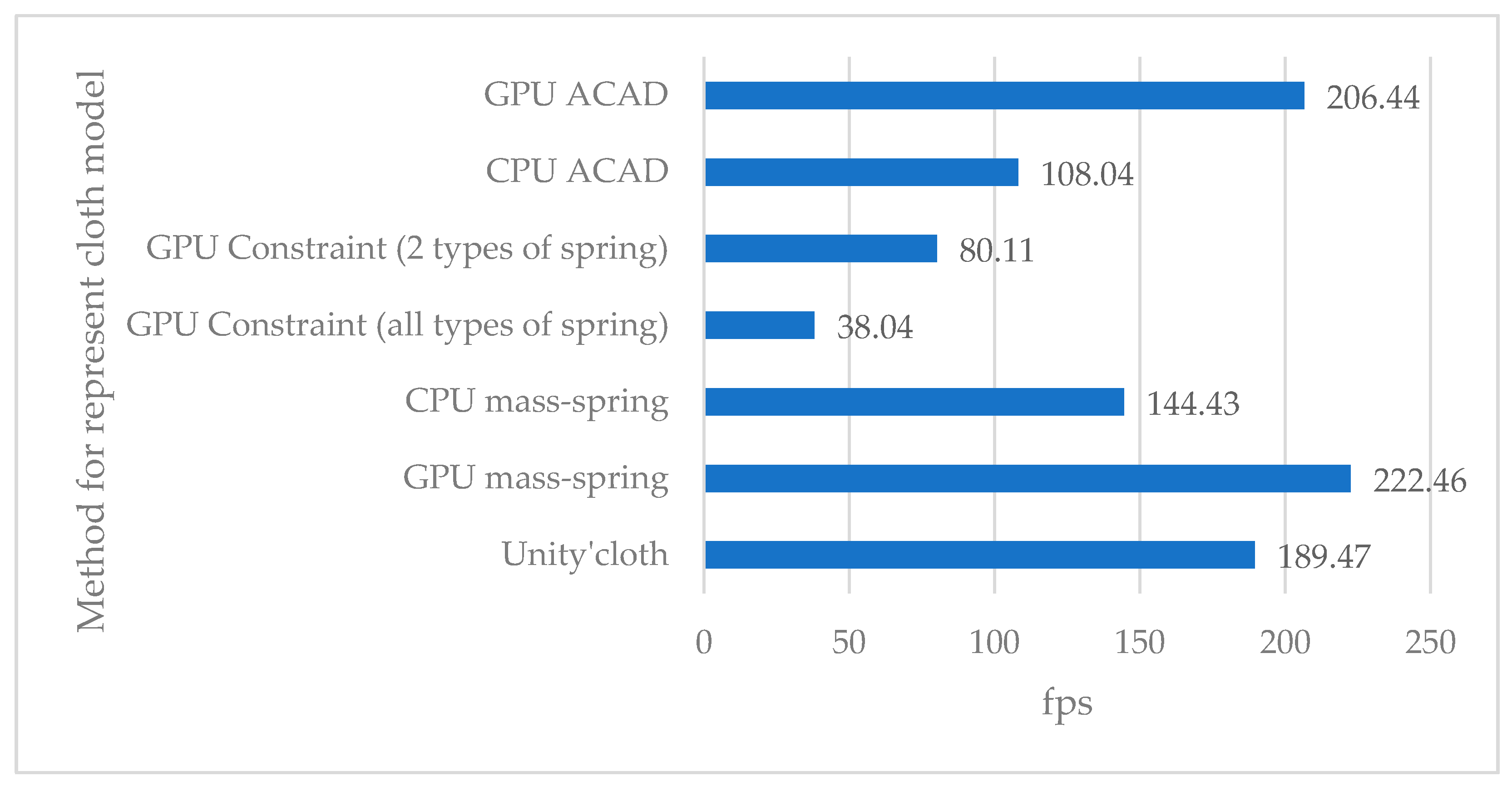
4.3. Performance Result

In this work, the vertical synchronization (VSync) is deactivated to compare the performance of the simulation measures by frames per second (fps). Since the measurement unit of performance (fps) defines how many average frames are rendered in a second, it shows how fast the algorithm runs. The proposed algorithm can be applied in VR and AR simulation, where the peak performance term of normal simulation is a performance in which simulation can be performed above 30 fps for general simulation, and above 60 fps for VR and AR simulation. Figure 7 compares the performance result between the CPU-based and GPU-based mass–spring system and Unity’s cloth object with different resolutions of the number of nodes n. However, Unity3D’s cloth object does not provide the number of springs, since the number of vertices is adapted to the types of the mesh. To make a fair comparison, the simulation performs 500 frames, while the average fps is calculated at the end of the simulation for different resolutions of the cloth model.

The peak performance result of the cloth simulation using Unity’s cloth object can achieve 65,636 nodes with 44.08 fps. Note that we use “Plane” mesh to represent the cloth object for Unity’s cloth method, and the limitation on vertices number is 65,536, but in the other method does not require “Plane” mesh, since it uses custom shading technique for rendering. On the other hand, the peak performance result of the cloth simulation using the CPU-based mass–spring system only achieves 9216 nodes in an average 44.83 fps, while the performance of GPU-based algorithm using compute shader obtains more than 200 fps in all cases.

Therefore, Figure 8 presents the maximum resolution of the GPU-based mass–spring cloth model to find the real-time performance. The peak performance of the mass–spring cloth model is about 34.81 fps for the cloth object that consists of 7,820,856 nodes. Compared to the CPU-based algorithm that uses serial process, the GPU-based algorithm delivers significantly better results, due to the massive parallelism of multi-thread that processes data in the GPU.

For these reasons, we further investigate the performance of cloth simulation using constraint enforcement that is implemented in Unity compute shader and measured in fps. Since the constraint enforcement algorithm is stable and accurate, we use only two types of spring (structural and shear), compared to the cloth model using all types of spring. Figure 9 illustrates the performance result of the cloth simulation using constraint enforcement in Unity with the different resolutions of the cloth model.

A cloth model using the constraint enforcement method with all types of springs obtains only 1156 nodes and 6598 springs with an average fps of 31.95. By reducing the level of spring to 3906, the performance achieves 66.06 fps on average for the same cloth model. On the other hand, the real-time performance of the cloth model using constraint enforcement algorithm can handle the resolution of the cloth with 1440 nodes and 5550 springs, and still achieve 44.25 fps. Since the constraint enforcement attempts to solve the large system in real-time, the maximum number of springs to be used for the cloth model is about 6000.

Since the cloth model using the GPU-based mass–spring system is extremely fast, but unstable when using a large time-step, the method of ACAD is applied to enhance the performance of the complex and large resolution of a cloth model. Figure 10 demonstrates the performance result of the cloth model with 1024 nodes and 5826 springs. The result shows that the constraint enforcement method can barely obtain the performance of cloth simulation in real-time, while the mass–spring system method outperforms the other methods with 222.46 fps on average. Alternatively, the ACAD method also confirms that it is a good choice for representing the cloth model, since it can obtain about 206.44 fps for the experimental cloth model.

The coefficient stiffness ks in Equation (1) defines the stiffness of the spring in a cloth model. Figure 11 shows the different behavior of the model using a GPU-based mass–spring system with 0.005 time-step.

In the constraint enforcement method, the cloth model using all spring types can reduce the performance of the simulation. Therefore, the cloth model using only two types of spring (structural and shear) is much faster for the same resolution of a model, but the cloth is stretched more than the model using all springs since the bend spring-type uses force to pull the other nodes, as shown in Figure 12.

Figure 13 illustrates the different behavior of the cloth model using our proposed method, and shows that the ACAD method is much faster than the constraint enforcement method. Since the spring force and constraint force are used, the spring coefficient ks affects the behavior of the cloth. The cloth model with large ks presents as hard cloth, while the cloth model with small ks presents as soft cloth.

The large time-step can also be applied to the cloth simulation based on the constraint enforcement method. However, the usage of all types of spring is more stable and accurate compared to the cloth without bend spring type. Figure 14 demonstrates the different behavior of the cloth model using the constraint enforcement method with a large time-step.

Figure 15 shows different behaviors of the cloth model using our proposed method and the mass–spring system method with large time-step. The cloth model using the mass–spring system method can blow up when a large time-step is used to perform the collision scenario. Therefore, the cloth model using the ACAD method will not blow up under the same conditions and will respond well to the collided object, but the cloth is stretched since the spring force is inaccurate at condition ks = 200.

Moreover, although the explicit Euler integration method is fast for estimating the next status of the velocity and position, it may cause much error in the result for large time-step compared to the Runge–Kutta method which provides more accurate estimation using extra computational costs. However, an implicit Euler method would help reducing the error much more than an explicit method in the presence of collision, but it requires more computational costs as well.

5. Conclusions

This research proposed a method to design and implement cloth simulation in Unity based on the mass–spring system, constraint enforcement method, and ADAC method with the parallel structure of compute shader kernel in GPU. Due to the usage of the parallel method in GPU, the performance of cloth simulation is much faster than CPU-based implementation. Additionally, the behavior results have shown that the mass–spring system method achieves stable and effective cloth behavior in the case where a small integration time-step and spring coefficient are used. Therefore, the constraint-based method provides stable and effective control of cloth behavior even with collision objects, and can be used with a large integration time-step. Using all types of springs to simulate a constraint enforcement cloth model is more stable and accurate than using only two types of springs. Our proposed method, ACAD, is used to reduce the computational burden of the cloth simulation to achieve stable and effective cloth behavior with large time-step during collision scenarios.

However, the limitation of the GPU-based mass–spring system approach is that it is necessary to manually pre-define the grid of the nodes. In the case where different models are used, the compute spaces should be modified to define the group of the thread in the GPU. Similarly, the constraint enforcement method requires the optimization of the size of the system matrix (COO matrix) to reduce the compute space in GPU. On the other hand, we utilize the atomic operation in the GPU to perform concurrent sum on the buffer data, but the usage of atomic operation is the main bottleneck of the whole operation in a simulation. Another limitation is that we experimented with the proposed simulation only with GPU NVIDIA GeForce GTX 1070; different GPUs may not perform our simulation well, due to the maximum number of threads per workgroup.

In future work, we will look for a method to optimize the performance result of the cloth simulation. In addition, we will apply parallel sum reduction to avoid the use of atomic operations in the simulation. The adaptive coefficient algorithm including machine learning and deep learning is required to study and predict the coefficient of the algorithm with regard to the cloth material. Furthermore, our simulation was implemented on Unity3D engine, which can be applied in the VR or AR application with real-time performance, due to the usage of parallel GPU.

References

1. Navarro-Hinojosa, O.; Ruiz-Loza, S.; Alencastre-Miranda, M. Physically-based visual simulation of the Lattice Boltzmann method on the GPU: A survey. J. Supercomput. 2018, 74, 3441–3467. [Google Scholar] [CrossRef]
2. Zhang, X.; Yu, X.; Sun, W.; Song, A. An Optimized Model for the Local Compression Deformation of Soft Tissue. KSII Trans. Internet Inf. Syst. 2020, 14, 671–686. [Google Scholar]
3. Zhao, P.; Liu, J.; Li, Y.; Wu, C. A spring-damping contact force model considering normal friction for impact analysis. Nonlinear Dyn 2021, 105, 1437–1457. [Google Scholar] [CrossRef]
4. Zhang, X.; Wu, H.; Sun, W.; Yuan, C. An Optimized Mass-spring Model with Shape Restoration Ability Based on Volume Conservation. KSII Trans. Internet Inf. Syst. 2020, 14, 1738–1756. [Google Scholar]
5. Tian, H.; Wana, C.; Zhana, X. A Realtime Virtual Grasping System for Manipulating Complex Objects. In Proceedings of the IEEE Conference on Virtual Reality and 3D User Interfaces (VR), Tuebingen/Reutlingen, Germany, 18–22 March 2018; pp. 1–2. [Google Scholar]
6. Chen, Z.; Huang, D.; Luo, L.; Wen, M.; Zhang, C. Efficient Parallel TLD on CPU-GPU Platform for Real-Time Tracking. KSII Trans. Internet Inf. Syst. 2020, 14, 201–220. [Google Scholar]
7. Li, J.; Guo, B.; Shen, Y.; Li, D. Low-power Scheduling Framework for Heterogeneous Architecture under Performance Constraint. KSII Trans. Internet Inf. Syst. 2020, 14, 2003–2021. [Google Scholar]
8. Unity. Available online: https://www.unity.com (accessed on 19 July 2021).
9. Obi Unified Particle Physics for Unity. Available online: http://obi.virtualmethodstudio.com (accessed on 19 July 2021).
10. Marinkovic, D.; Zehn, M. Survey of Finite Element Method-Based Real-Time Simulations. Appl. Sci. 2019, 9, 2775. [Google Scholar] [CrossRef] [Green Version]
11. Lamecki, A.; Dziekonski, A.; Balewski, L.; Fotyga, G.; Mrozowski, M. GPU-Accelerated 3D Mesh Deformation for Optimization Based on the Finite Element Method. Radioengineering 2017, 26, 924–929. [Google Scholar] [CrossRef]
12. Volino, P.; Magnenat-Thalmann, N.; Faure, F. A simple approach to nonlinear tensile stiffness for accurate cloth simulation. ACM Trans. Graph 2009, 28, 105. [Google Scholar] [CrossRef] [Green Version]
13. Weber, D.; Bender, J.; Schnoes, M.; Stork, A.; Fellner, D. Efficient GPU data structures and methods to solve sparse linear systems in dynamics applications. Comput. Graph. Forum 2013, 32, 16–26. [Google Scholar] [CrossRef]
14. Chen, Z.; Zheng, X.; Guan, T. Structure-Preserving Mesh Simplification. KSII Trans. Internet Inf. Syst. 2020, 14, 4463–4482. [Google Scholar]
15. Müller, M.; Heidelberger, B.; Hennix, M.; Ratcliff, J. Position based dynamics. J. Vis. Commun. Image Represent. 2007, 18, 109–118. [Google Scholar] [CrossRef] [Green Version]
16. Eberhardt, B.; Etzmuß, O.; Hauth, M. Implicit-explicit schemes for fast animation with particle systems. In Computer Animation and Simulation; Springer: Vienna, Austria, 2000; pp. 137–151. [Google Scholar]
17. Provot, X. Deformation constraints in a mass-spring model to describe rigid cloth behavior. In Graphics Interface; Canadian Information Processing Society: Quebec City, QC, Canada, 1995; pp. 147–154. [Google Scholar]
18. Georgii, J.; Westermann, R. Mass-spring systems on the GPU. Simul. Model. Pract. Theory 2005, 13, 693–702. [Google Scholar] [CrossRef]
19. Mosegaard, J.; Sorensen, T.S. GPU accelerated surgical simulators for complex morphology. In Proceedings of the IEEE VR 2005, Bonn, Germany, 12–16 March 2005; pp. 147–153. [Google Scholar]
20. Hong, M.; Welch, S.; Choi, M.H. Intuitive control of dynamic simulation using improved implicit constraint enforcement. In Asian Simulation Conference; Springer: Berlin/Heidelberg, Germany, 2004; pp. 315–323. [Google Scholar]
21. Goldenthal, R.; Harmon, D.; Fattal, R.; Bercovier, M.; Grinspun, E. Efficient Simulation of Inextensible Cloth. In ACM SIGGRAPH 2007 Papers; Association for Computing Machinery: New York, NY, USA, 2007; p. 49-es. [Google Scholar]
22. Baraff, D.; Witkin, A. Large steps in cloth simulation. In Proceedings of the 25th Annual Conference on Computer Graphics and Interactive Techniques 1998, Orlando, FL, USA, 19–24 July 1998; pp. 43–54. [Google Scholar]
23. Hong, M.; Choi, M.H.; Jung, S.; Welch, S.; Trapp, J. Effective constrained dynamic simulation using implicit constraint enforcement. In Proceedings of the 2005 IEEE International Conference on Robotics and Automation; IEEE: New York, NY, USA, 2005; pp. 4531–4536. [Google Scholar]
24. Va, H.; Lee, D.; Hong, M. Parallel algorithm of conjugate gradient solver using OpenGL compute shader. J. Korea Soc. Comput. Inf. 2021, 26, 1–9. [Google Scholar]
25. Park, H.; Baek, N. Developing an Open-Source Lightweight Game Engine with DNN Support. Electronics 2020, 9, 1421. [Google Scholar] [CrossRef]
26. Compute Shader Overview. Available online: https://docs.microsoft.com/en-us/windows/win32/direct3d11/direct3d-11-advanced-stages-compute-shader (accessed on 19 July 2021).
27. Steinberger, M.; Zayer, R.; Seidel, H.P. Globally homogeneous, locally adaptive sparse matrix-vector multiplication on the GPU. In Proceedings of the International Conference on Supercomputing 2017, Chicago, IL, USA, 14–16 June 2017; pp. 1–11. [Google Scholar]
28. Steinberger, M.; Derlery, A.; Zayer, R.; Seidel, H.P. How naive is naive SpMV on the GPU? In Proceedings of the IEEE High-Performance Extreme Computing Conference (HPEC), Waltham, MA, USA, 13–15 September 2016; pp. 1–8. [Google Scholar]
Figure 1. Mass–spring model for cloth simulation.
Applsci 11 08255 g001
Figure 2. The compute space dimension of the kernel in Unity.
Applsci 11 08255 g002
Figure 3. Scheme of accessing buffer through the index of the thread.
Applsci 11 08255 g003
Figure 4. Flowchart of cloth simulation using constraint enforcement method with compute shader in Unity.
Applsci 11 08255 g004
Figure 5. Flowchart of cloth simulation using the ACAD method with compute shader in Unity.
Applsci 11 08255 g005
Figure 6. Collision detection between node and spherical object.
Applsci 11 08255 g006
Figure 7. The performance comparison of cloth simulation using Unity’s cloth, CPU-based, and GPU-based mass–spring system.
Applsci 11 08255 g007
Figure 8. The performance result of cloth simulation using the GPU-based mass–spring system measured in fps.
Applsci 11 08255 g008
Figure 9. The performance result of cloth simulation using GPU-based constraint enforcement with and without bend spring and measured in fps.
Applsci 11 08255 g009
Figure 10. Performance comparison of the cloth simulation using the different methods.
Applsci 11 08255 g010
Figure 11. The behavior of the cloth using the mass–spring system method with different ks.
Applsci 11 08255 g011
Figure 12. Comparison of the behavior of the cloth model using the constraint enforcement method with and without bend spring, and using a 0.005 time-step.
Applsci 11 08255 g012
Figure 13. Comparison of the behavior of the cloth model using the ACAD method with different coefficient ks, and using a 0.005 time-step.
Applsci 11 08255 g013
Figure 14. Comparison of the behavior of the cloth model using the constraint enforcement method with and without bend spring, and using a 0.016 time-step.
Applsci 11 08255 g014
Figure 15. Comparison on the behavior of the cloth model using the mass–spring system method and the ACAD method with a 0.016 time-step, 200 ks.
Applsci 11 08255 g015