
Design of Autonomous Mobile Robot for Cleaning in the Environment with Obstacles


Abstract
:1. Introduction
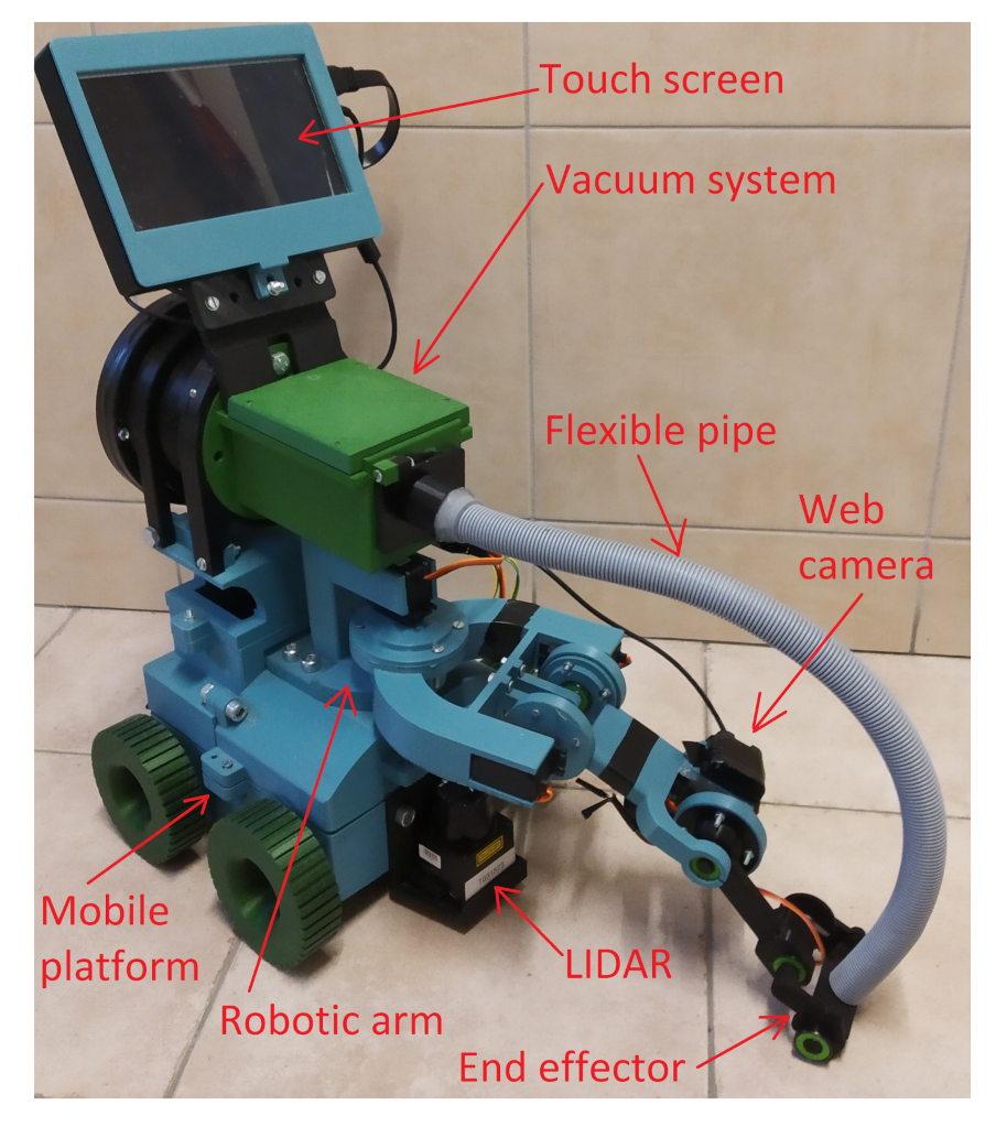
2. Mechanical Design and Electronics Parts
- Lightweight parts.
- Suitable for 3D printing.
- Strength of PLA material.
- Ease of assembly.
- Robotic arm.
- Vacuum system.
- Mobile platform.
2.1. Robotic Arm
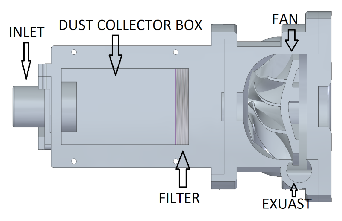
2.2. Vacuum System
2.3. Mobile Platform
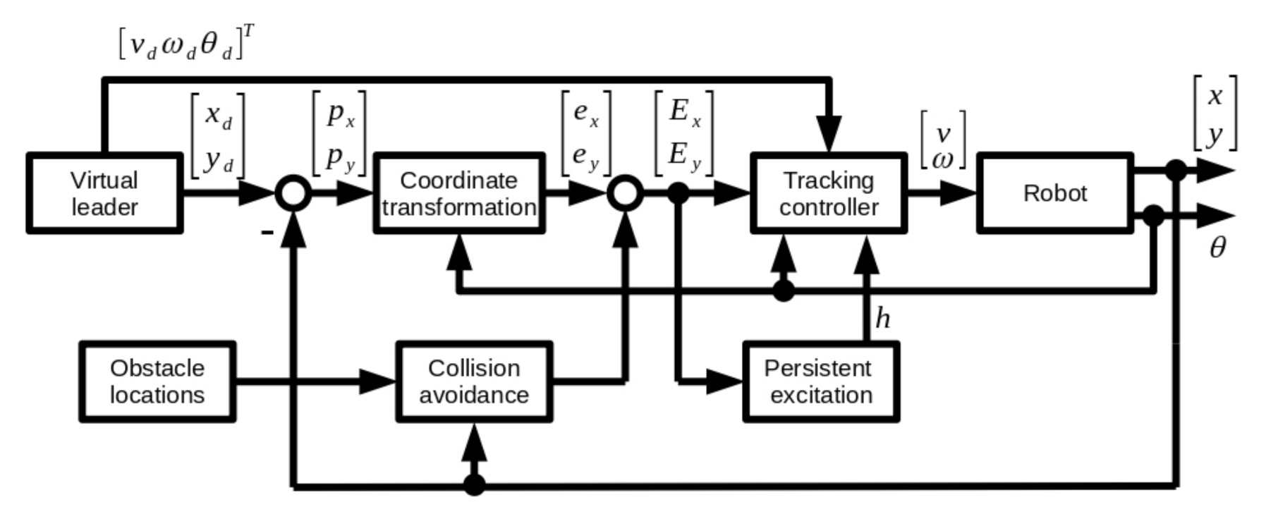
3. Control Algorithm
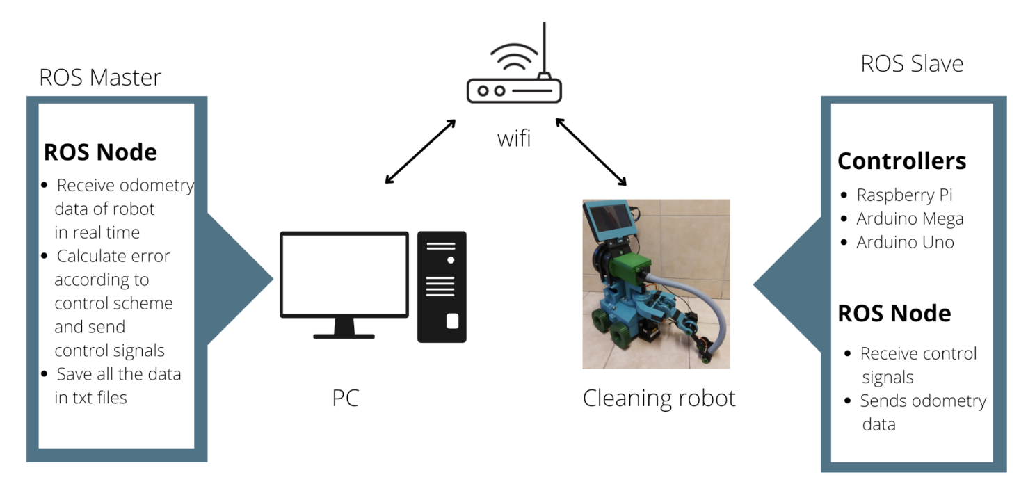
4. Methodology
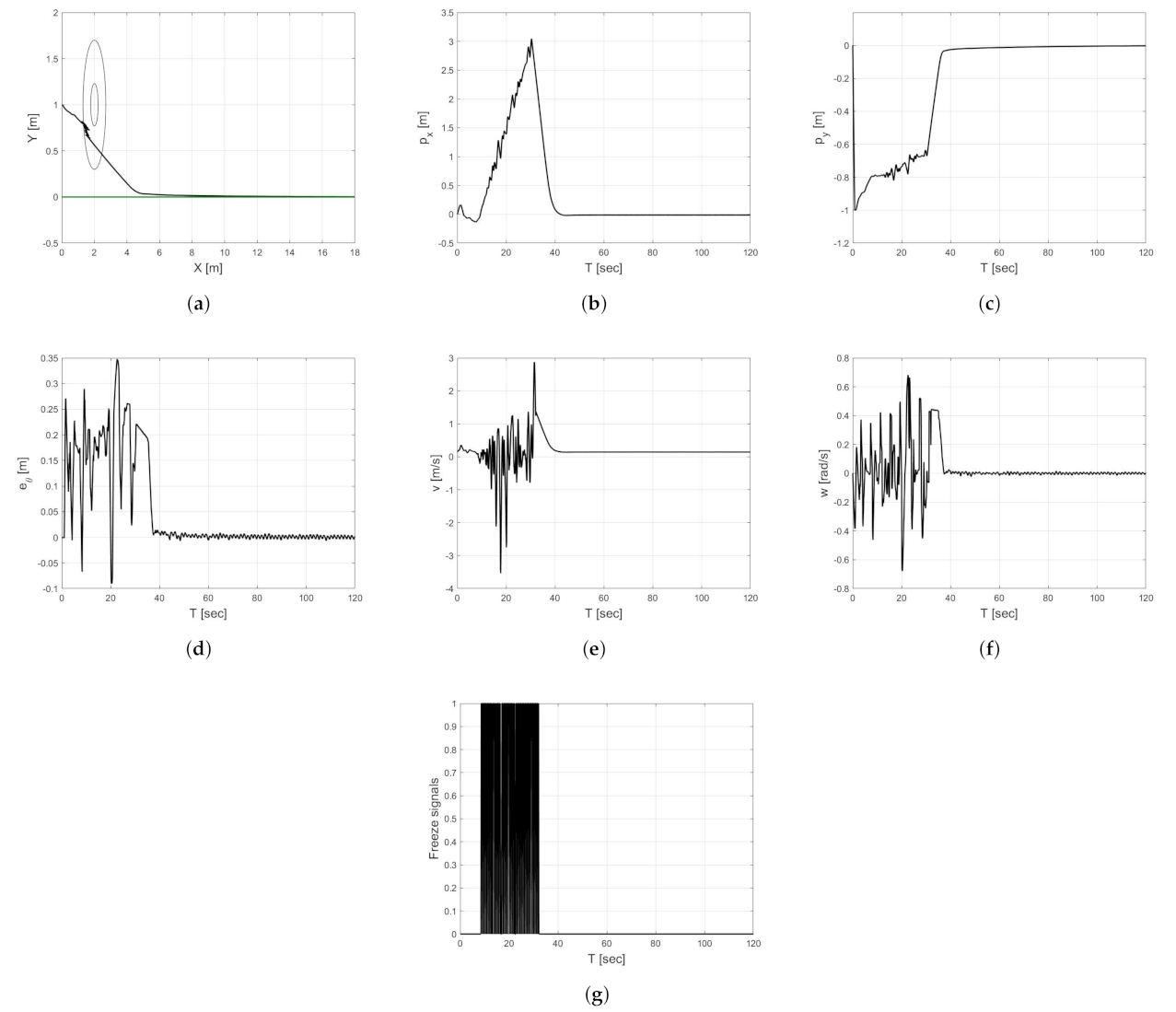
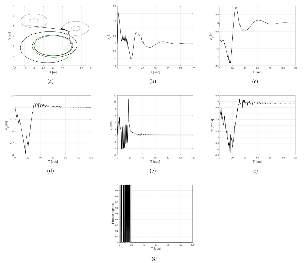
5. Experiment Results
5.1. Experiment 1
5.2. Experiment 2
6. Conclusions
Author Contributions
Funding
Acknowledgments
Conflicts of Interest
References
- Prassler, E.; Ritter, A.; Schaeffer, C. A Short History of Cleaning Robots. Auton. Robots 2000, 9, 211–226. [Google Scholar] [CrossRef]
- Asafa, T.B.; Afonja, T.M.; Olaniyan, E.A.; Alade, H.O. Development of a vacuum cleaner robot. Alex. Eng. J. 2018, 57, 2911–2920. [Google Scholar] [CrossRef]
- Murdan, A.P.; Ramkissoon, P.K. A smart autonomous floor cleaner with an Android-based controller. In Proceedings of the 3rd International Conference on Emerging Trends in Electrical, Electronic and Communications Engineering (ELECOM), Balaclava, Mauritius, 25–27 November 2020; Volume 57, pp. 235–239. [Google Scholar] [CrossRef]
- Hasan, K.M.; Nahid, A.A.; Reza, K.J. Path planning algorithm development for autonomous vacuum cleaner robots. In Proceedings of the International Conference on Informatics, Electronics and Vision (ICIEV), Dhaka, Bangladesh, 23–24 May 2014; Volume 57, pp. 1–6. [Google Scholar] [CrossRef]
- Prayash, H.A.S.H.; Shaharear, M.R.; Islam, M.F.; Islam, S.; Hossain, N.; Datta, S. Designing and Optimization of An Autonomous Vacuum Floor Cleaning Robot. In Proceedings of the IEEE International Conference on Robotics, Automation, Artificial-Intelligence and Internet-of-Things (RAAICON), Dhaka, Bangladesh, 29 November–1 December 2019; pp. 25–30. [Google Scholar] [CrossRef]
- Vaussard, F.; Fink, J.; Bauwens, V.; Rétornaz, P.; Hamel, D.; Dillenbourg, P.; Mondada, F. Lessons learned from robotic vacuum cleaners entering the home ecosystem. Robot. Auton. Syst. 2014, 62, 376–391. [Google Scholar] [CrossRef] [Green Version]
- Ulrich, I.; Mondada, F.; Nicoud, J.-D. Autonomous vacuum cleaner. Robot. Auton. Syst. 1997, 19, 233–245. [Google Scholar] [CrossRef] [Green Version]
- Kowalczyk, W.; Kozłowski, K. Trajectory tracking and collision avoidance for the formation of two-wheeled mobile robots. Bull. Pol. Acad. Sci. 2019, 67, 915–924. [Google Scholar] [CrossRef]
- Garcia-Sillas, D.; Gorrostieta-Hurtado, E.; Vargas, J.E.; Rodrí-guez-Reséndiz, J.; Tovar, S. Kinematics modeling and simulation of an autonomous omni-directional mobile robot. Ing. Investig. 2015, 35, 74–79. [Google Scholar] [CrossRef] [Green Version]
- Martínez-Prado, M.; Rodríguez-Reséndiz, J.; Gómez-Loenzo, R.; Herrera-Ruiz, G.; Franco-Gasca, L. An FPGA-Based Open Architecture Industrial Robot Controller. IEEE Access 2018, 6, 13407–13417. [Google Scholar] [CrossRef]
- Montalvo, V.; Estévez-Bén, A.A.; Rodríguez-Reséndiz, J.; Macias-Bobadilla, G.; Mendiola-Santíbañez, J.D.; Camarillo-Gómez, K.A. FPGA-Based Architecture for Sensing Power Consumption on Parabolic and Trapezoidal Motion Profiles. Electronics 2020, 57, 1301. [Google Scholar] [CrossRef]
- Khatib, O. Real-Time Obstacle Avoidance for Manipulators and Mobile Robots. Int. J. Robot. Res. 1986, 5, 90–98. [Google Scholar] [CrossRef]
- Dimarogonasa, D.V.; Loizoua, S.G.; Kyriakopoulos, K.J.; Zavlanosb, M.M. A Feedback Stabilization and Collision Avoidance Scheme for Multiple Independent Non-point Agents. Bull. Pol. Acad. Sci. 2006, 67, 229–243. [Google Scholar] [CrossRef]
- Filippidis, I.; Kyriakopoulos, K.J. Adjustable Navigation Functions for Unknown Sphere Worlds. In Proceedings of the IEEE Conference on Decision and Control and European Control Conference (CDCECC), Orlando, FL, USA, 12–15 December 2011; pp. 4276–4281. [Google Scholar] [CrossRef]
- Roussos, G.; Kyriakopoulos, K.J. Decentralized and Prioritized Navigation and Collision Avoidance for Multiple Mobile Robots. Distrib. Auton. Robot. Syst. Springer Tracts Adv. Robot. 2013, 83, 189–202. [Google Scholar] [CrossRef]
- Roussos, G.; Kyriakopoulos, K.J. Completely Decentralised Navigation of Multiple Unicycle Agents with Prioritisation and Fault Tolerance. In Proceedings of the IEEE Conference on Decision and Control (CDC), Atlanta, GA, USA, 15–17 December 2010; pp. 1372–1377. [Google Scholar]
- Roussos, G.; Kyriakopoulos, K.J. Decentralized Navigation and Conflict Avoidance for Aircraft in 3-D Space. IEEE Trans. Control. Syst. Technol. 2012, 20, 1622–1629. [Google Scholar] [CrossRef]
- Mastellone, S.; Stipanovic, D.; Spong, M. Formation control and collision avoidance for multi-agent non-holonomic systems: Theory and experiments. Int. J. Robot. Res. 2008, 27, 107–126. [Google Scholar] [CrossRef]
- Kowalczyk, W.; Kozłowski, K. Leader-Follower Control and Collision Avoidance for the Formation of Differentially-Driven Mobile Robots. In Proceedings of the 23rd International Conference on Methods and Models in Automation and Robotics MMAR, Miedzyzdroje, Poland, 27–30 August 2018. [Google Scholar]
- Do, K. Formation Tracking Control of Unicycle-Type Mobile Robots with Limited Sensing Ranges. IEEE Trans. Control. Syst. Technol. 2008, 16, 527–538. [Google Scholar] [CrossRef] [Green Version]
- Kowalczyk, W.; Kozłowski, K.; Tar, J.K. Trajectory tracking for multiple unicycles in the environment with obstacles. In Proceedings of the 19th International Workshop on Robotics in Alpe-Adria-Danube Region RAAD, Budapest, Hungary, 24–26 June 2010; pp. 451–456. [Google Scholar] [CrossRef]
- Guldner, J.; Utkin, V.I.; Hashimoto, H.; Harashima, F. Tracking gradients of artificial potential fields with non-holonomic mobile robots. In Proceedings of the 1995 American Control Conference-ACC’95, Seattle, WA, USA, 21–23 June 1995; Volume 4, pp. 2803–2804. [Google Scholar] [CrossRef]
- Zhou, L.; Li, W. Adaptive Artificial Potential Field Approach for Obstacle Avoidance Path Planning. In Proceedings of the Seventh International Symposium on Computational Intelligence and Design, Hangzhou, China, 13–14 December 2014; pp. 429–432. [Google Scholar] [CrossRef]
- Loria, A.; Dasdemir, J.; Alvarez Jarquin, N. Leader—Follower Formation and Tracking Control of Mobile Robots Along Straight Paths. IEEE Trans. Control Syst. Technol. 2016, 57, 727–732. [Google Scholar] [CrossRef] [Green Version]
- De Wit, C.C.; Khennouf, H.; Samson, C.; Sordalen, O.J. Nonlinear Control Design for Mobile Robots. In Recent Trends in Mobile Robots; World Scientific Publishing Company: Singapore, 1994; pp. 121–156. [Google Scholar]
- Michałek, M.; Kozłowski, K. Vector-Field-Orientation Feedback Control Method for a Differentially Driven Vehicle. IEEE Trans. Control Syst. Technol. 2010, 18, 45–65. [Google Scholar] [CrossRef]
- Kowalczyk, W.; Michałek, M.; Kozłowski, K. Trajectory tracking control with obstacle avoidance capability for unicycle-like mobile robot. Bull. Pol. Acad. Sci. Tech. Sci. 2012, 60, 537–546. [Google Scholar] [CrossRef] [Green Version]


| Joint Number | Servo Name | Quantity | Torque |
|---|---|---|---|
| Joint 1 | Tower Pro SG-5010 | 1 | 6.5 kg × cm |
| Joint 2 | Feetech FS5115M | 2 | 15.5 kg × cm |
| Joint 3 | Tower Pro SG-5010 | 1 | 6.5 kg × cm |
| Joint 4 | Tower Pro SG-90-micro | 1 | 1.8 kg × cm |
| S.No | Component Name | Specification |
|---|---|---|
| 1 | ESC, skywalker | Input- 2–4 s Lipo, continous current 50 A |
| 2 | Brushless motor, iFlight XING | 2750 KV, max current 50.03 A |
| 3 | Lipo battery | 11.1v, 50C, 5000 mAh |
| S.No | Component Name | Quantity | Specification |
|---|---|---|---|
| 1 | Motor Driver, L298N | 2 | Maximum current 2A |
| 2 | Arduino Mega | 1 | 54 digital input/output pins |
| 3 | Arduino Uno | 1 | 14 digital input/output pins |
| 4 | Raspberry Pi 4 | 1 | 2 GB RAM |
| 5 | Battery | 1 | 6 V, 12 Ah |
| 6 | DC motor- Pololu 99:1 Metal | 4 | Integrated 48 CPR quadrature encoder |
| gearmotor 25D×66L | 4741.44 CPR, Torque-15 kg/cm | ||
| 14 digital input/output pins |
Publisher’s Note: MDPI stays neutral with regard to jurisdictional claims in published maps and institutional affiliations. |
© 2021 by the authors. Licensee MDPI, Basel, Switzerland. This article is an open access article distributed under the terms and conditions of the Creative Commons Attribution (CC BY) license (https://creativecommons.org/licenses/by/4.0/).
Share and Cite
Joon, A.; Kowalczyk, W. Design of Autonomous Mobile Robot for Cleaning in the Environment with Obstacles. Appl. Sci. 2021, 11, 8076. https://doi.org/10.3390/app11178076
Joon A, Kowalczyk W. Design of Autonomous Mobile Robot for Cleaning in the Environment with Obstacles. Applied Sciences. 2021; 11(17):8076. https://doi.org/10.3390/app11178076
Chicago/Turabian StyleJoon, Arpit, and Wojciech Kowalczyk. 2021. "Design of Autonomous Mobile Robot for Cleaning in the Environment with Obstacles" Applied Sciences 11, no. 17: 8076. https://doi.org/10.3390/app11178076
APA StyleJoon, A., & Kowalczyk, W. (2021). Design of Autonomous Mobile Robot for Cleaning in the Environment with Obstacles. Applied Sciences, 11(17), 8076. https://doi.org/10.3390/app11178076