Abstract
In this work, the use of adaptive filters for reducing forecast errors produced by a Regional Climate Model (RCM) is investigated. Seasonal forecasts are compared against the reanalysis data provided by the National Centers for Environmental Prediction. The reanalysis is used to train adaptive filters based on the Recursive Least Squares algorithm in order to reduce the forecast error. The K-means unsupervised learning algorithm is used to obtain the number of filters to employ from the climate variables. The proposed approach is applied to some climate variables such as the meridional wind, zonal wind, and the geopotential height. The forecast is produced by the Eta RCM at 40-km resolution in a domain covering most of Brazil. Results show that the proposed approach is capable of reducing the forecast errors, according to evaluation metrics such as normalized mean square error, maximum absolute error, and maximum normalized absolute error, thus improving the seasonal climate forecasts.
1. Introduction
Climate forecasts aim at providing the most probable evolution of the climate in a future time window. Numerical methods are applied to model and solve the physics laws that govern atmospheric circulation [1]. An atmospheric model is a tool to predict the evolution of climate conditions for a certain region [2,3].
The Eta Regional Climate Model (RCM) has provided seasonal forecasts over South America since 2002 [4]. The Eta model [5,6] has been employed by the Brazilian National Institute for Space Research (INPE) since 1996 [7] for high-resolution numerical weather forecasts. The Eta model employs as prognostic variables: air temperature, zonal and meridional wind components, specific humidity, surface pressure, turbulent kinetic energy, soil humidity and temperature, and liquid or ice water in clouds [8,9]. Climate forecasts using any numerical method/model (such as the Eta) will generally differ from the observed climatic conditions.
To reduce forecast errors, one normally carries out statistical bias correction of climate model outputs by using methods based on distribution mapping, power transformation, local intensity, and linear scaling [10,11,12,13]. These methods adjust the statistics of the climate forecast such as mean, variance, and distribution matching; other methods proceed by attempting to adjust wet days probability [14]. In addition, these studies show that approaches based on quantile mapping with gamma distribution result in better performance on RCM bias correction. In [15], the authors compared the quantile mapping (QM) with gamma distribution adjustment against power transformation, considering the Eta RCM precipitation. They concluded that the former method is more appropriate for daily precipitation bias correction. In the literature, we found bias correction being performed in the frequency domain, usually by employing Discrete Fourier Transform. This framework treats both univariate [16,17] and multivariate [18] cases. The frequency-domain bias correction comprises several timescales simultaneously, whereas the QM techniques are restricted to specific timescales as shown in [19,20,21]. Recently, in [22], the authors used discrete wavelet transforms to correct systematic bias in spectral attributes from raw General Circulation Model simulations results, more specifically, on global mean sea level and the Arctic sea-ice extent.
This work aims to investigate the possibility of improving the quality of climate forecasts by filtering the predicted climate variables using adaptive filters. The adaptive filters are applied to the Eta seasonal forecasts. In this work, we consider the design of filters for postprocessing of the prognostic variables in order to reduce forecast errors. The filters are designed for different spatial regions using adaptive algorithms and are also inherently capable of processing different timescales simultaneously. The spatial regions are defined through a clustering algorithm. Therefore, in our proposal, temporal variability is treated by adaptive filtering and spatial variability is treated by clustering. Our work innovates by employing adaptive filtering techniques for RCM bias correction.
The NCEP (National Centers for Environmental Prediction) provides a dataset aiming to be a bona fide portrait of the observed climatic conditions. This dataset is known as NCEP reanalysis, from the term NCEP/CFSR (NCEP/Climate Forecast System Reanalysis). It is constructed from a combination of forecasts and observed meteorological data, which are then processed and fused into a regular grid to produce the NCEP reanalysis [23]. These data can be used to verify the forecast skill of meteorological models.
The filter coefficients are adjusted and adapted, comparing the Eta model forecasts against the NCEP reanalysis data. This can result in filtered prognoses having both a temporal behavior and statistical characteristics that are more similar to the observed conditions than the original forecasts.
Therefore, we investigate the validity and the effectiveness of different setups using adaptive filters to improve climate forecasts. In this paper, we employ the output of the Eta model at 40-km resolution and compare it against the NCEP reanalysis at 38-km resolution. The reanalysis dataset was remapped onto the Eta grid in order to enable comparisons. The chosen filter-updating technique refers to the RLS (Recursive Least-Squares) algorithm [24]. Different grid cells are grouped depending on the climate forecast variables during the forecast period. For data partitioning and clustering, we use the K-means algorithm [25,26]. This unsupervised learning algorithm is used to automatically choose the number of filters employed for forecast improvement in the geographical domain. Seminal work was introduced in [27], and we extend it here by comprising more climate forecast variables, presenting an improved adaptive filter algorithm, and using additional evaluation metrics.
The paper is organized as follows. Section 2 presents some details on the climate forecast data used in this work, more specifically on its volumetric characteristic and the volume discretization (grid), and also on the geographic region of interest. Section 3 shows how the adaptive filters are employed to reduce the climate forecast error. Following, Section 4 describes the proposed methodology, which comprises the data grid adjustment approach between Eta RCM and NCEP data sets, the clustering technique applied to the climate time series, and the evaluation of the clustering quality that is used to decide the number of filters to employ in a given region. The methodology also comprises a brief presentation of the RLS algorithm used for adaptive filtering and how to evaluate the performance of the proposed climate forecast error reduction approach. Section 5 presents the experimental setup and numerical results, and discusses the performance of the proposed method for the reduction of RCM forecast deviations. Section 6 ends with the conclusions.
2. Seasonal Climate Forecasts
Weather and climate forecasts differ basically on the forecast period, and the integration length employed in the numeric solution. Weather forecasts extend for about ten (10) days. In contrast, climate forecasts encompass the analysis of a longer time scale (months or years) of meteorological variables that are treated statistically. Both forecasts are interested in temperature, geopotential height, wind, specific humidity, surface pressure, precipitation, clouds, among other variables.
The climate forecasts considered in this work are within the region inside the dashed rectangle in Figure 1. This region is located within the latitudes 6 S and 30 S and the longitudes 33 W and 83 W, covering most of Brazil. The forecast dataset is produced by the Eta climate model using a spatial resolution of 40 km.
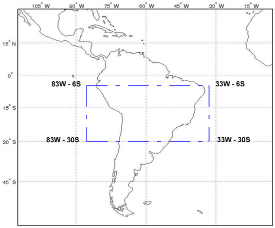
Figure 1.
Limits of the region considered for adjusting the Eta-40-km climate forecast using as reference the NCEP reanalysis.
Regional climate forecast requires initial conditions in the model domain and lateral boundary conditions along its contour. The initial conditions in the region must describe the observed atmospheric state so that they may be a reliable scenario for the atmospheric variables to evolve. Meanwhile, the contour conditions (which are necessary for regional climate models) describe the state of the atmosphere in the region’s border from a coarser model dataset. These conditions drive the regional model domain, which in turn provides a smaller scale climate forecasts that is dynamically downscaling [2,3]. The Eta Regional Climate Model outputs used in this study are derived from ten-year seasonal reforecasts [28], which have been shown to add value over the driver coarse global model forecasts, especially during the rainy seasons. The evaluation was based on the temporal correlation between forecasts and observations of precipitation seasonal anomaly. In addition, the regional forecasts reproduce the average upper and lower level winds in different seasons of the year.
However, regional climate forecasts are not completely accurate and differ from the observed climate. The differences have several origins and tend to increase as the integration time (the forecast time range) advances. There are approximations such as those inherent to the physics of the model or the initial conditions errors (inside the region and along the borders). All these aspects contribute to produce climate forecast inaccuracies, i.e., errors. While the initial conditions may affect short- and medium-term prognoses (days to weeks), the lateral boundary conditions along the borders affect the long-term (months and years) prognosis of regional climate [3,29]. For example, the prognostics from Eta-40-km are used as contour conditions for even higher resolution models such as the Eta-15-km, affecting numerical simulation results.
Eta outputs prognoses with a six-hour time interval. They may be envisioned as 3-dimension data that evolve with time since each prognostic variable is spatially sampled using latitude, longitude, and altitude coordinates. Therefore, a temporal sequence of the predicted values of a given climatic variable in a region of interest can be understood as a discrete volumetric signal. There is a 3D matrix (a tensor) for each climate variable that evolves depending on the time index n. Let denote this tensor. It contains the value of the variable in each volumetric cell at time 1, 2, ⋯, L—L being the prognosis interval.
The elements in the tensor are indexed by their spatial positions; consequently, the i-th element in is the value of the variable x at the coordinates at time n. Consequently, represents the time-series (signal) containing the values of the prognosis for the variable x at the i-th cell over time. We use the term ”cell“ to refer to a specific position (latitude, longitude, and height). If is used for the vectorization operation, then
is the vector correspondent to the time series .
In the presented work, the i-th cell signal enters a filter with impulse response aiming at producing an output to present better accordance with the observed data than does. A possible approach to turn the resulting convolution, , more similar to than , is by means of adaptive filtering. Filters are designed by adaptively considering clusters of coordinates instead of designing a filter for each cell alone. However, before obtaining the filters for the adjustment of the climate forecast, we discuss how adaptive filters can be used for designing them.
3. Forecast Error Reduction by Adaptive Filtering
If is the time series of a forecast variable at a given cell, the reduction of RCM forecast error by filtering process aims at obtaining a filtered version , mathematically described by the so-called difference equation
where are the N-order filter coefficients, and are the output and input signals, and l is the coefficient index that also indicates the l-th past sample of the input signal. The n-th iteration of this process is illustrated in Figure 2. The sliding windows passes over previous samples of the input signals—over in the figure—and the filter order is . In this case, we consider a digital filter with finite impulse response (FIR) [30] that produces the output as in Equation (2).
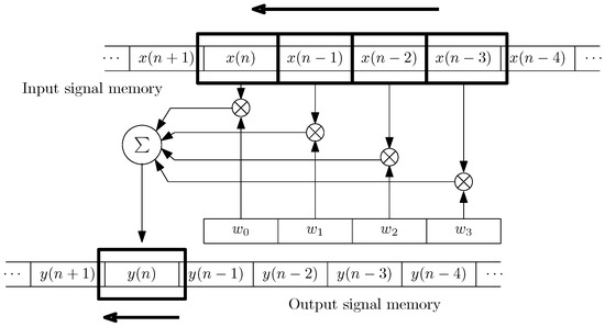
Figure 2.
Filtering process employed to reduce climate forecast errors.
In the proposed approach, the filter is designed using adaptive filtering techniques. The general framework of adaptive filtering is shown in Figure 3, where n is the iteration number, denotes the forecast time series, denotes the adapted filter output signal, and is the NCEP reanalysis considered the reference time series [24]. The error signal is computed by subtracting from , which subsidies the adaptive algorithm to appropriate updating of the filter coefficients. The coefficients are adjusted iteratively to reduce the error. Hence, the filter is adaptive.
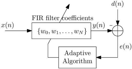
Figure 3.
General configuration of adaptive filtering.
The core idea is to find the optimum filter that, when it is applied to the forecast climate time series, its output becomes more adherent to the observational data—in this case, the NCEP reanalysis. It is expected that the adapted filter based on past data from Eta RCM forecast and NCEP reanalysis should lead to forecast accuracy improvement of the Eta model’s future forecasts. One notes the dependence on past data for the filter training process. For the adaptive filter design, several factors need to be considered, such as filter length and adaptive algorithm.
In addition, the statistical behavior of climate times series depends on the geographic location of the evaluated region. As a starting point, one highlights that it is unlikely to find one single optimum filter for the whole domain. Hence, data partitioning and clustering are required for adequate filter adaption. In doing so, one obtains filters that are applicable at specific spatial domains (forecast cells), and the filters inherently consider prognostic evolution, a temporal aspect. We apply the K-means, an unsupervised learning algorithm, to obtain the number of filters to use. The next section describes the specific methodology that we adopt.
4. Proposed Framework for Climate Forecast Error Reduction
We employ adaptive filters to adjust the prognostic series of the regional climate model and improve its accuracy. Figure 4 describes the methodology employed to obtain the filters that improve the accuracy of climate forecasts. The volumetric data at a given point (lat, long, alt) forms a time series. Filter adaption requires training. Time series corresponding to different cells are grouped using the K-means algorithm [25] to produce training sets containing enough samples so that robust statistics are available. Clustering and filter training apply at year YYYY, and the resulting filters adjust the prognoses for the following year (YYYY + 1).
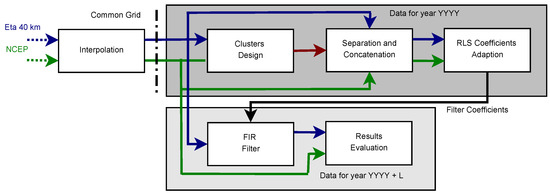
Figure 4.
Basic methodology for filter adaption in order to improve the forecast skill of climate models. The Eta forecast and the NCEP reanalysis are adjusted to the same grid. Then, in the Clusters Design block, unsupervised learning is employed to clusters cells presenting similar statistics. The time-series of the climate variables in each cluster are serialized in the Separation and Concatenation block. The resulting signals are used to adjust filter coefficients of the FIR filter that postprocesses the climate forecast cells on the time dimension, aiming at reducing forecast errors. Filter adaption uses the RLS (Recursive Least-Squares) algorithm.
4.1. Data Grid Adjustment
The spatial grid of the Eta model output at 40-km resolution differs from the NCEP reanalysis grid. While the Eta provides a 61 × 126 elements matrix in the region of interest, the NCEP reanalyses provide a matrix having 49 × 101 elements for the same region. This is due to the difference in their spatial resolution; while the Eta model employs 0.4 resolution, NCEP employs 0.5. Consequently, grid adjustment between both datasets is necessary. Both datasets were scaled through interpolation to 0.1, leading to a 244 × 504-point matrix.
4.2. Climate Series Clustering
The K-means algorithm [25] is employed to cluster the grid time series from different cells. Clustering reduces the number of filters to be trained. One trains a filter for each clustered time series (a group of cells) instead of one filter for each time series (one cell), increasing the quantity of data available to adapt each filter. Using the K-means, one clusters the time series of different cells according to the (vector) distance between them. At each iteration, one evaluates the partitioning quality and reassigns the time series within the clusters so that they are more similar within a cluster and more different among clusters.
Let be the set of Z elements to be clustered. Consider K clusters , for and , each cluster is represented by a centroid , . K-means clusters the elements in using the distances to the centroids—that is, is assigned to the -th cluster if , where is the Euclidean distance between two vectors (For vectors and , i.e., , is the n-th coordinate of .). After assigning the elements to the clusters, each cluster centroid is updated as the arithmetic mean of its elements. The mean is an appropriate metric since it can be representative of magnitude of the variable in the season.
At the first iteration, K elements in are randomly selected as centroids [25,31]. The process in the paragraph above is iterated until a predefined number of iterations is reached or the process stabilizes in terms that very small variations of assignments and centroids occur. Let be the number of elements in cluster k, the total clustering distance within cluster k is
and the total clustering distortion (considering all clusters) is
Small changes in between successive iterations represent small changes in the clusters, meaning that the assignment of the time-series to clusters stabilizes.
The problem one must address is to find the best number of clusters K for a given dataset. This is an unsupervised learning problem. We do not need only to assign the time series within clusters to minimize the total distortion but also to discover the appropriate number of clusters for the dataset. To investigate this, we use the “Validity” index
Above,
which is the sum of the distances inside each cluster and
returns the smaller distance between cluster centroids. The K-means minimizes iteratively all the , maximizing also the distances between different cluster centroids [31]. Consequently, for a given K, it minimizes intra while maximizing inter, resulting in minimizing Validity. As a result, the smaller the value of Equation (5), the better the clustering. This way, one learns the appropriate number of filters to be designed for the considered geographical region and time frame.
To define the clusters, one uses the means of the climate forecast variables in each cell during the forecast period. This approach attempts to group cells presenting similar climates over time and not similar forecast errors. The latter could lead to grouping cells presenting very similar error behavior but from different climates. This could hamper the moving average model in Equation (2) and Figure 3 to follow the time series behavior over time.
For the clustering process, we define the vector , where the first subscript is used to indicate the forecast variable, the second indicates the cell, and i refers to ordered pair . More precisely, for the first subscript, 1 denotes the meridional wind (m/s), 2 denotes the zonal wind (m/s), and 3 denotes the geopotential height; the overline indicates the average over time n, i.e., .
Once we learn the number of filters to be employed, the filters that the time series within each cluster for forecast error reduction need to be learned. However, in this case, one can use supervised learning from the forecast error in previous time series. This is accomplished using adaptive filtering. The time series within each cluster are randomly concatenated in time, and the resulting series is used to adapt the correspondent filter using the Recursive Least Squares algorithm.
4.3. Recursive Least Squares Adaptive Filters
We employ the Recursive Least Squares (RLS) algorithm for the adaptive filters. The RLS algorithm aims to minimize the MSE (Mean Squared Error) at the filter output. It converges rapidly if the eigenvalues of the input signal correlation matrix are reasonably spread and present good performance when the input signal presents fast amplitude changes [24].
Let be the input signal deterministic autocorrelation matrix
and be the deterministic cross-correlation between the input and the desired signal
in that is the input information vector, is the reference signal sample, and is the so-called forgetting factor, i.e., an exponential weighting factor that should be chosen between 0 and 1.
At the n-th iteration of the RLS, it produces the updated filter coefficients vector by means of
Although the computational cost of the matrix inversion is too high, strategies to avoid it leading to viable algorithms exist; for more details, see [24].
There is one adaptive filter for each cluster resulting from the K-means whose input is obtained from the RCM Eta forecast time series for the cells in the cluster. Meanwhile, the reference signal is composed of the NCEP reanalysis time series of the cells within the cluster.
4.4. Performance Evaluation
The reduction in climate forecasts errors using adaptive filters can be evaluated by comparing the error between the Eta forecast and the NCEP reanalysis before and after it passes through the filter. Note that this applies only to the adjusted forecast; in Figure 4, the data for the year YYYY + L.
To evaluate the performance, we employ some error indices: the maximum error, its normalized maximum error, and the NMSE (normalized mean squared error). They are given by
Above, is the error between the series from the Eta-40-km forecasts, original and filtered, and the reference series , from the NCEP reanalysis. Each time series corresponds to the temporal change of a climate variable of each volumetric cell in the climate model.
Effectiveness in Reducing RCM Forecast Deviations
The maximum error value as given in Equation (11) and its normalized counterpart (Equation (12)) analyze the largest error at the cells over time; while evaluates the extreme cases, evaluates their relative impacts. They depend on the error at a given sample (time) in a given cell; thus, they analyze local errors in the volume-time/cell-sample space (at a given cell and time). On the other hand, the NMSE in Equation (13) compares the energy/sample of the error against the energy/sample of the reference time series. Hence, it evaluates the error in the entire time series. The smaller the error is, the better is the adjusted time series in a mean squared sense, meaning that the distance between the adjusted forecast and the observed climate is reduced. However, none of them consider the entire climate model domain.
In order to evaluate the performance of the forecast adjustment in the entire climate model domain, we define the Effectiveness Rate of RCM forecast deviation reduction as
where is the total number of time series and denotes the number of time series for which a reduction in RCM forecast deviation is observed. This can be computed for each one of the error metrics in Equations (12) and (13).
Since we have one climate numerical simulation per year, we also compute the Mean Effectiveness Rate, defined as
where is the quantity of years and is the deviation reduction effectiveness rate of the i-th year.
5. Experiments
5.1. Climate Variables
In this work, we have focused on the major variables that drive the large scale of atmosphere and climate variability. The use of geopotential height is equivalent to the use of air temperature, through the hydrostatic relation. The surface pressure is derived from wind convergence and temperature of the atmospheric column. Variables such as moisture, cloud, turbulent kinetic energy, and soil conditions are strongly dependent on model parameterization schemes, which are additional sources of uncertainties in numerical models. Therefore, for a proof of concept, this work has focused on the geopotential height and the zonal and meridional winds. The 500-hPa level is critical as it contains atmospheric waves that drive the development of phenomena at the surface level, such as extratropical cyclones and fronts. The 250-hPa level contains the position of upper-level jets or storm tracks that play important roles in the development of large-scale waves in the atmosphere. Therefore, the current work has chosen to focus on two atmospheric levels: 250-hPa and 500-hPa. We use the forecasts for the period between 2001 to 2010. Each forecast comprises the period from 17 December to 30 April. Consequently, each series corresponds to a 133-day forecast period with four (4) samples per day, yielding a time series of 533 samples long. These correspond to austral summer period. This is the rainy season over most of South America. Further details on the construction of this data set can be found in [28].
5.2. Learning Clusters
Considering the averages of the three climate variables—the meridional wind (m/s), zonal wind (m/s), and the geopotential height (in geopotential meters)—at the pressure levels 250 hPa and 500 hPa, the quality of the clustering is evaluated using the validity index (see Equation (5)). We calculated the validity index for a number of clusters ranging from 2 to 24. After exhaustive tests, this range proved to be wide enough to achieve low validity and avoid small clusters. The result is shown in Figure 5. The number of clusters resulting in the lowest validity was , which results in an average of 6400 time series per cluster inside the considered region within 6 S–30 S and 33 W–83 W. For each of the clusters, one obtains a different filter using the RLS adaptive filter.
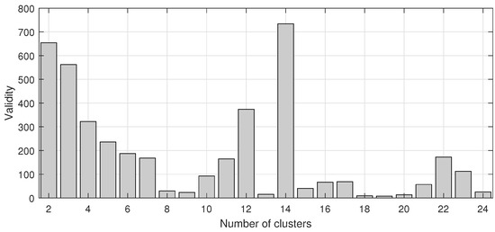
Figure 5.
Evaluation of the number of clusters by means of the Validity index.
We employ K-means due to its simplicity and wide use [26,32]. It is important to mention that the K-means are not applied on the time series containing the climate forecasts but on their time averages, reducing the dimension of the clustering problem. Figure 6 shows the clusters provided by K-means. One can note that they are reasonably linked with our previous knowledge of climate resemblance in different subregions within the considered region. Other clustering approaches could be attempted based on self-organizing maps using directly the data points (a cell over the considered time-frame presenting several climate variables). One could use dimensional reduction mappings such as principal component analysis, independent component analysis, and other nonlinear dimension reduction methods to map the data points for an alternative clustering space, which might provide better results. However, as we develop in the sequel, k-means clustering proved effective for training adaptive filters for reducing climate forecast errors.
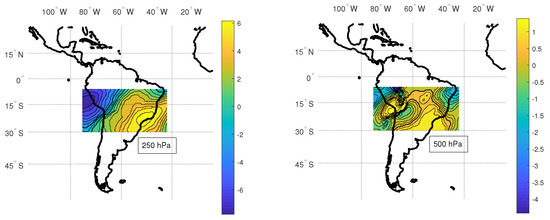
Figure 6.
Clustering results via K-means for meridional wind (m/s) produced by Eta RCM at 250 hPa and 500 hPa in the forecast domain, considering .
5.3. Adaptive Filter Configuration
We test adaptive filters of several lengths to adjust the 40-km Eta forecast. The filters’ order is set to be 4, 8, 16, and 32 samples, which correspond to one, two, four, and eight days of forecast, respectively. The results are averaged over ten (10) trials/rounds. At each round, one randomly sorts the time series concatenation sequence for filter adaption. These provide more reliable results and analyses of the proposed adjustment for the climate forecast. In the experiments, the RLS algorithm employs . However, as aforementioned, before filter adaption (design), one needs to effectively cluster the prognosis cells.
5.4. Capturing Spatial and Temporal Variability
The proposed framework treats the spatial variability through the clustering procedure and the temporal variability through adaptive filtering. Figure 6 illustrates the clustering results of the meridional wind variable at 250 and 500-hPa levels in the forecast domain. The color-bar indicates the centroids of the cluster regions. One can note more homogeneous and smooth clusters at 250 hPa than at 500 hPa. This is expected since the atmosphere at 500 hPa level height is nearer to the earth’s surface, which produces a spatial structure due to surface features such as the continents and mountains.
Figure 7 presents the 250-hPa meridional wind for a time slice of the forecast, which started on 13 December 2001. This shows the temporal variability of the time series. The filtered data approaches the reference NCEP data and shows the reduction of the forecast errors.
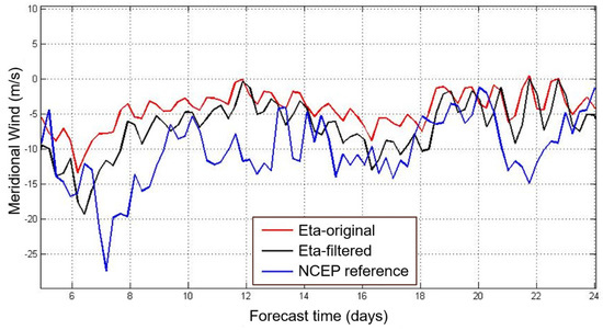
Figure 7.
Meridional wind time series at 250 hPa produced by the Eta RCM (Eta-original), its filtered version (Eta-filtered), and the NCEP reference data.
5.5. Results
Regarding the experimental setup, we compute ER (see Equation (14)) for three deviation metrics, considering data from years 2001 to 2010 (), at two pressure levels (250 hPa and 500 hPa), while designing/adapting filters of different lengths 4, 8, 16, and 32 (1, 2, 4, and 8 days, respectively, as discussed in Section 5.3). The number of clusters used in K-means is fixed at 19 (as discussed in Section 5.2). The combination of these setup variables generates an amount of ER data spread in a three-dimensional domain associating an axis to each one of the deviation metrics considered herein. Let NMSE, , and be the ordered series containing the ER data of the corresponding deviation metric in the different years of each time series, at each pressure level of each climate variable and value of N. By computing the correlation coefficient among the ER values of NMSE, , and , we can verify that since their correlation is around 0.5 and 0.6, as shown in Table 1, these results reveal different aspects. Remark that the poor cross-correlation among these error metrics proves that none of them should to be discarded in the proposed framework performance evaluation, since they evaluate distinct aspects of the systematic error between Eta RCM and the observational data.

Table 1.
Correlations between effectiveness rates for NMSE, , and .
To assess the performance of the proposed strategy for RCM deviation reduction, we plot the obtained ER data by combining simulation years and filter orders with respect to these three deviation metrics, as illustrated in Figure 8 and Figure 9. These three-dimensional graphs present the ERs for each of the deviation metrics considered for the four filter lengths. The graph analysis is carried out separately at each pressure level, 250 hPa and 500 hPa. The more the cloud points are concentrated in the top-right corner, the better is the performance on reducing the RCM forecast deviation according to the three error metrics simultaneously. The better performance at 500 hPa than at 250 hPa is an important result. Variables at 500 hPa are closer to the surface than 250 hPa; therefore, the improvement of the 500-hPa variables can contribute more to the improvement of the forecasts near the surface. At the 250-hPa level, the climate variables exhibit longer wavelengths than at 500-hPa [33]; therefore, the filter acted more effectively at the 500-hPa level where more climate variability is found.
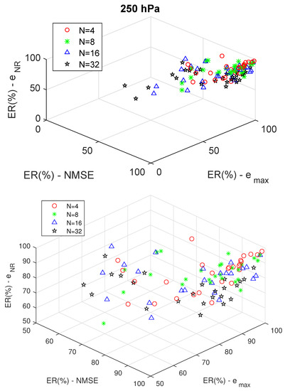
Figure 8.
Effectiveness rate of RCM forecast deviation reduction at 250 hPa with different filter orders (above), and a larger view with values greater than .
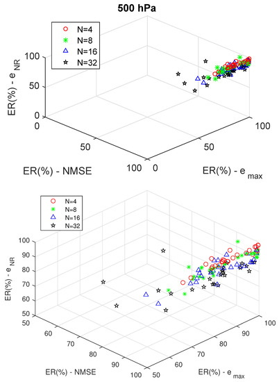
Figure 9.
Effectiveness rate of RCM forecast deviation reduction at 500 hPa with different filter orders (above), and a larger view with values greater than .
In addition, at both pressure levels, the ER performance decreases as the filter order increases. This becomes evident when we compute the centroids (averages) and dispersion of the cloud points separated by filter order. Table 2 contains the MER (%) and the standard deviation () of the error metrics for each pressure level and filter order (N). Note that the larger MER and the smaller dispersion (marked in boldface) occur for the four-coefficient filter at the two pressure levels. It is important to highlight that the filter performs the convolution over the entire time series produced by the Eta RCM; therefore, it is applied for error correction. The filter does not produce a forecast. There is a 6-h interval between each value of the time series; therefore, the four-coefficient filter, comprising a 24-h time period, removes the diurnal cycle, which is a strong signal in meteorological time series. The 6-h interval is the sampling interval availability of the Eta RCM forecasts data set. It should be noted that a four-coefficient filter refers to a one-day forecast. Moreover, the NMSE leads to a larger MER centroid and smaller dispersion than and . This is expected given that the filter is adapted in the least-square sense for the whole time series length, i.e., on average.
Table 2.
Centroid (MER) and dispersion () of effectiveness rates for different filter orders at 250 hPa and 500 hPa.
From the preceding results, we now fix the filter order at and the number of clusters at and evaluate the MER with respect to the error metrics NMSE, , and , separating the analysis into climate variables: meridional wind, zonal wind, and geopotential height. The results are shown in Table 3. At 250 hPa, meridional wind provides the best MER performance with respect to the three forecast deviation metrics. At 500 hPa, all studied climate variables show equivalent MER performance with respect to NMSE and , whereas for the geopotential height, one achieves the best MER performance with respect to .
Table 3.
Mean effectiveness rates (%) of climate variables at 250 hPa and 500 hPa, considering a four-coefficient filter and 19 clusters.
6. Conclusions
This paper proposed a postprocessing approach to reduce forecast deviations of the Eta regional climate model by using adaptive filters. The correction of forecast deviation depends on comparisons between past model forecasts and reanalysis data. These data are applied to the well-known RLS (Recursive Least-Squares) algorithm to obtain the filter.
There are many cells within the geographic domain of climate forecast. Each cell presents a set of climate variable time series. Therefore, the K-means clustering algorithm is employed to learn the number of filters adapted in the model domain. The criterion for the clusters is the average climate in the cells.
The fraction of climate forecast cells where the error between the prognosis (Eta RCM) and the observed (NCEP) reduces the effectiveness rate (ER) is used to evaluate the proposal. One computes the ER for three error metrics: the normalized mean square error, the maximum absolute error, and the absolute normalized error.
The proposed procedure was tested in a region comprising most of Brazil, within 6 S–30 S and 33 W–83 W. The results show that the proposed method can achieve high effectiveness rates (ER) in reducing forecast deviations of the Eta RCM, mainly with a four-coefficient filter that corresponds to a one-day time period. Moreover, at 500 hPa, we could obtain better ER performance than at 250 hPa. This is an important and useful result, as the 500-hPa level climate variables affect more closely the variables near the surface, where people live.
Author Contributions
Conceptualization, M.P.T., L.L. and S.C.C.; methodology, M.P.T., A.R.F. and L.L.; software, A.R.F. and M.P.T.; validation, A.R.F and M.P.T.; writing—original draft preparation, M.P.T. and L.L.; writing—review and editing, M.P.T., L.L. and S.C.C. All authors have read and agreed to the published version of the manuscript.
Funding
This study was financed in part by Coordenação de Aperfeiçoamento de Pessoal de Nível Superior—Brasil (CAPES) Finance Code 001, by Conselho Nacional de Desenvolvimento Científico e Tecnológico (CNPq) no. 306757/2017-6 and by Fundação Carlos Chagas Filho de Amparo à Pesquisa do Estado do Rio de Janeiro (FAPERJ).
Institutional Review Board Statement
Not applicable.
Informed Consent Statement
Not applicable.
Conflicts of Interest
The authors declare no conflict of interest.
References
- Holton, J.R.; Hakim, G.J. An Introduction to Dynamic Meteorology; Academic Press: Cambridge, MA, USA, 2012; Volume 88. [Google Scholar]
- Castro, C.L.; Pielke, R.A.; Leoncini, G. Dynamical downscaling: Assessment of value retained and added using the Regional Atmopsheric Modeling System (RAMS). J. Geophys. Res. Atmos. 2005, 110, 1–21. [Google Scholar] [CrossRef]
- Laprise, R.; de Elía, R.; Caya, D.; Biner, S.; Lucas-Picher, P.; Diaconescu, E.; Leduc, M.; Alexandru, A.; Separovic, L. Challenging some tenets of Regional Climate Modelling. Meteorol. Atmos. Phys. 2008, 100, 3–22. [Google Scholar] [CrossRef]
- Chou, S.C.; Bustamante, J.F.; Gomes, J. Evaluation of Eta Model seasonal precipitation forecasts over South America. Nonlinear Process. Geophys. 2005, 12, 537–555. [Google Scholar] [CrossRef] [Green Version]
- Black, T.L. The new NMC mesoscale Eta model: Description and forecast examples. Weather. Forecast. 1994, 9, 265–278. [Google Scholar] [CrossRef] [Green Version]
- Mesinger, F.; Janjić, Z.I.; Ničković, S.; Gavrilov, D.; Deaven, D.G. The step-mountain coordinate: Model description and performance for cases of Alpine lee cyclogenesis and for a case of an Appalachian redevelopment. Mon. Weather. Rev. 1988, 116, 1493–1518. [Google Scholar] [CrossRef] [Green Version]
- Chou, S.C. Modelo regional Eta. Climanálise 1996, 1, 27–29. Available online: http://climanalise.cptec.inpe.br/~rclimanl/boletim/cliesp10a/27.html (accessed on 27 May 2021). (In Portuguese).
- Mesinger, F.; Chou, S.C.; Gomes, J.L.; Jovic, D.; Bastos, P.; Bustamante, J.F.; Lazic, L.; Lyra, A.A.; Morelli, S.; Ristic, I.; et al. An upgraded version of the Eta model. Meteorol. Atmos. Phys. 2012, 116, 63–79. [Google Scholar] [CrossRef] [Green Version]
- Mesinger, F.; Veljovic, K.; Chou, S.C.; Gomes, J.; Lyra, A. The Eta model: Design, use, and added value. In Topics in Climate Modeling; InTech: London, UK, 2016. [Google Scholar]
- Piani, C.; Haerter, J.O.; Coppola, E. Statistical bias correction for daily precipitation in regional climate models over Europe. Theor. Appl. Climatol. 2010, 99, 187–192. [Google Scholar] [CrossRef] [Green Version]
- Jakob Themeßl, M.; Gobiet, A.; Leuprecht, A. Empirical-statistical downscaling and error correction of daily precipitation from regional climate models. Int. J. Climatol. 2011, 31, 1530–1544. [Google Scholar] [CrossRef]
- Teutschbein, C.; Seibert, J. Bias correction of regional climate model simulations for hydrological climate-change impact studies: Review and evaluation of different methods. J. Hydrol. 2012, 456, 12–29. [Google Scholar] [CrossRef]
- Berg, P.; Feldmann, H.; Panitz, H.J. Bias correction of high resolution regional climate model data. J. Hydrol. 2012, 448, 80–92. [Google Scholar] [CrossRef]
- Maraun, D. Bias correcting climate change simulations—A critical review. Curr. Clim. Chang. Rep. 2016, 2, 211–220. [Google Scholar] [CrossRef] [Green Version]
- Tschöke, G.V.; Kruk, N.S.; de Queiroz, P.I.B.; Chou, S.C.; de Sousa Junior, W.C. Comparison of two bias correction methods for precipitation simulated with a regional climate model. Theor. Appl. Climatol. 2017, 127, 841–852. [Google Scholar] [CrossRef]
- Pierce, D.W.; Cayan, D.R.; Maurer, E.P.; Abatzoglou, J.T.; Hegewisch, K.C. Improved bias correction techniques for hydrological simulations of climate change. J. Hydrometeorol. 2015, 16, 2421–2442. [Google Scholar] [CrossRef]
- Nguyen, H.; Mehrotra, R.; Sharma, A. Correcting for systematic biases in GCM simulations in the frequency domain. J. Hydrol. 2016, 538, 117–126. [Google Scholar] [CrossRef] [Green Version]
- Nguyen, H.; Mehrotra, R.; Sharma, A. Correcting systematic biases across multiple atmospheric variables in the frequency domain. Clim. Dyn. 2019, 52, 1283–1298. [Google Scholar] [CrossRef]
- Mehrotra, R.; Sharma, A. A multivariate quantile-matching bias correction approach with auto-and cross-dependence across multiple time scales: Implications for downscaling. J. Clim. 2016, 29, 3519–3539. [Google Scholar] [CrossRef]
- Johnson, F.; Sharma, A. A nesting model for bias correction of variability at multiple time scales in general circulation model precipitation simulations. Water Resour. Res. 2012, 48. [Google Scholar] [CrossRef] [Green Version]
- Haerter, J.; Hagemann, S.; Moseley, C.; Piani, C. Climate model bias correction and the role of timescales. Hydrol. Earth Syst. Sci. 2011, 15, 1065–1079. [Google Scholar] [CrossRef] [Green Version]
- Kusumastuti, C.; Jiang, Z.; Mehrotra, R.; Sharma, A. A signal processing approach to correct systematic bias in trend and variability in climate model simulations. Geophys. Res. Lett. 2021, 48, e2021GL092953. [Google Scholar] [CrossRef]
- Kistler, R.; Collins, W.; Saha, S.; White, G.; Woollen, J.; Kalnay, E.; Chelliah, M.; Ebisuzaki, W.; Kanamitsu, M.; Kousky, V.; et al. The NCEP–NCAR 50–year reanalysis: Monthly means CD–ROM and documentation. Bull. Am. Meteorol. Soc. 2001, 82, 247–267. [Google Scholar] [CrossRef]
- Diniz, P.S. Introduction to Adaptive Filtering. In Adaptive Filtering; Springer: Berlin/Heidelberg, Germany, 2020; pp. 1–8. [Google Scholar]
- Han, J.; Pei, J.; Kamber, M. Data Mining: Concepts and Techniques; Elsevier: Amsterdam, The Netherlands, 2011. [Google Scholar]
- Friedman, J.; Hastie, T.; Tibshirani, R. The Elements of Statistical Learning; Springer Series in Statistics New York; Springer: Berlin/Heidelberg, Germany, 2001; Volume 1. [Google Scholar]
- Freitas, A.R.; Tcheou, M.P.; Lovisolo, L.; Chou, S.C. Filtragem adaptativa para a redução de desvios em séries temporais de previsão numérica climática. In Proceedings of the Simpósio Brasileiro de Telecomunicações e Processamento de Sinais, Juiz de Fora, Brazil, 1 September 2015. (In Portuguese). [Google Scholar]
- Chou, S.C.; Dereczynski, C.; Gomes, J.L.; Pesquero, J.F.; AVILA, A.; Resende, N.C.; Alves, L.F.; Ruiz-Cardenas, R.; Souza, C.R.D.; Bustamante, J.F.F. Ten-year seasonal climate reforecasts over South America using the Eta Regional Climate Model. An. Acad. Bras. Ciênc. 2020, 92. [Google Scholar] [CrossRef] [PubMed]
- Davies, T. Lateral boundary conditions for limited area models. Q. J. R. Meteorol. Soc. 2014, 140, 185–196. [Google Scholar] [CrossRef]
- Diniz, P.S.R.; Da Silva, E.A.B.; Netto, S.L. Digital Signal Processing: System Analysis and Design; Cambridge University Press: Cambridge, UK, 2010. [Google Scholar]
- Lovisolo, L.; Da Silva, E. Uniform distribution of points on a hyper-sphere with applications to vector bit-plane encoding. IEE Proc. Vision Image Signal Process. 2001, 148, 187–193. [Google Scholar] [CrossRef]
- Wu, X.; Kumar, V.; Quinlan, J.R.; Ghosh, J.; Yang, Q.; Motoda, H.; McLachlan, G.J.; Ng, A.; Liu, B.; Philip, S.Y.; et al. Top 10 algorithms in data mining. Knowl. Inf. Syst. 2008, 14, 1–37. [Google Scholar] [CrossRef] [Green Version]
- Hoskins, B.; Pearce, R. Large-Scale Dynamical Processes in the Atmosphere; Academic Press: Cambridge, MA, USA, 1983. [Google Scholar]
Publisher’s Note: MDPI stays neutral with regard to jurisdictional claims in published maps and institutional affiliations. |
© 2021 by the authors. Licensee MDPI, Basel, Switzerland. This article is an open access article distributed under the terms and conditions of the Creative Commons Attribution (CC BY) license (https://creativecommons.org/licenses/by/4.0/).