Experimental Study on the Ventilation Resistance Characteristics of Paddy Grain Layer Modelled with Response Surface Methodology

Abstract

The ventilation resistance of air flow through rice grain layers is one of the key parameters affecting drying uniformity as well as the energy consumption of the drying process. In order to reveal the variation of characteristics of the ventilation resistance with paddy grain moisture content, the air velocity and the bed layer depth are needed. A second order model was fitted to pressure drop using the response surface methodology and the results are compared with those of the Ergun model. The results showed that the pressure drop increases with the increase of paddy grain moisture content, air velocity and the bed layer depth, and the interactions between the air velocity and the bed layer depth have the most significant influence on the pressure drop. Moreover, a second-order polynomial pressure drop model based on RSM was established and compared with the Ergun model. The results showed that the pressure drop model established by RSM is similar to that of the Ergun model.

1. Introduction

The pressure drop of the grain bed layer is the key parameter for designing and optimizing the structure of the drying chamber, and it is also one of the most important references for selecting the power of a fan [1,2]. During the drying process, owing to the bed layer porosity as well as the air viscosity, there must be a pressure drop when the air flows through the bed layer. A high-pressure drop may make it difficult for the air to flow through the bed layer and further lead to the increase of non-uniformity of the drying process, while a low-pressure drop may lead to wasting the power of the fan [3]. Accordingly, it is necessary to find out a reasonable pressure drop under the premise of ensuring product quality and maintaining a reasonable power demand of the fan.

In the last few decades, researchers have done many studies on the ventilation resistance of the grain bed layer by applying the traditional pressure drop models [4,5,6,7]. For example, Gunasekaran and Jackson [8] conducted an experiment on the flow resistance of sorghum bed layer by applying the Ergun model, the resistance of sorghum moisture content of 16.5, 18.5, and 23 %w.b. were determined under the grain bed depth of 150 to 1200 mm with the airflow ranges of 0.05 to 0.3 m/s. The results showed that the resistance of airflow increases with the increase of air velocity and bed layer depth, while resistance increases with the decrease of moisture content. Li et al. [9] applied the Shedd model to simulate the flow resistance of the hot air flow through the paddy grain bed layer; they found that the flow resistance of the hot air increases with the increase of hot air velocities. Zhang et al. [10] investigated the pressure drop of the air (with velocity ranges of 0.1 to 0.6 m/s) flow through the bed layer with depth ranges of 100 to 1000 mm, and found that the simulation accuracy of the pressure drop using Ergun model is reliable only when the air velocity is under 0.2 m/s. It can be summarized from the above analyses that the flow resistance of the grain bed layer are mainly determined by the traditional models and the characteristics of the air flow resistance are investigated by using single factor test. Though the works provided some valuable references for guiding the practical production, the air flow resistance prediction accuracy based on traditional models should be further improved and the interaction of the parameters on the flow resistance should be further investigated.

Respond surface methodology (RSM) is one of the most effective modeling tools to investigate the interactions of two or more variables on the responses, which is widely adopted to optimize the process parameters in the agriculture field [11,12]. Zeng et al. [13] conducted an experimental study on the vacuum drying extraction technology of konjac glucomannan using RSM, and an artificial neuron network (ANN) was also adopted and then compared with the RSM. The results showed that the model established by RSM is slightly better than that of an ANN. In order to improve the dynamic performance of orchard ditching fertilizer and to avoid resonance, Liu et al. [14] adopted the RSM to optimize the structure of the rack of orchard ditching–fertilizer machine. The results showed that the optimized structure has a better first-order modal frequency of 38.31 Hz than that of the traditional structure, and the optimized frequency is far away from the input frequency (35 Hz) of a tractor, indicating that the frequency of the structure optimized by RSM can avoid the resonance. Moreover, Kowalczyk et al. [15] adopted the RSM to optimize the production process of a micro-elemental feed additive for laying hens, the most favorable enrichment conditions of the process were determined by the model established by the RSM. It can be summarized that the RSM is widely used in the agricultural field, and it can be also adopted to model the ventilation resistance of paddy grain layer.

The present work adopted the RSM to model the ventilation resistance of paddy grain layer. In detail, an experiment followed by Box–Behnken Design was conducted to investigate the influences of the independent variable including paddy grain moisture content (Mc), air velocity (v_air), and paddy layer depth (L) on the pressure drop (Δp). The influences of the single factor as well as the interactions between any two independent variables on Δp were investigated and a ternary quadratic model for Δp was established and compared with the traditional Ergun model.

2. Materials and Methods

To fully understand the variation rules of ventilation resistance of the air flowing through paddy grain layer and further specify the optimization strategy for deep bed paddy drying process. A laboratory-scale experimental test was conducted based on the engineering application consideration; the detailed analysis steps are as follows.

2.1. Materials

The paddy grains sample with initial moisture content of 12.2 %w.b. are purchased from a local farmer at Leizhou Guangdong Province, China. The samples are, respectively manual humidified to 13.6 %w.b., 14.8 %w.b., 16.2 %w.b., 17.8 %w.b., 18.9 %w.b., 21.3 %w.b., 22.9 %w.b., 24.5 %w.b., and 25.6 %w.b. according to the methodology introduced in the literature [16]. Additionally, the prepared samples are sealed in plastic bags and stored in a refrigerator at approximately 4 °C for about 48 h prior to the experiments [13].

2.2. Experimental Apparatus

As can be seen from Figure 1, the apparatus mainly consists of 6 parts including the centrifugal fan, frequency converter, air supply duct, screen mesh, test pipeline, and the fixing bracket. There are 10 pressure taps with a diameter of 10 mm on the test pipeline, the height of the test pipeline is 1100 mm, and the distance between any two adjacent pressure taps is 100 mm. Moreover, there is one air velocity tap closed to connection between the test pipeline and air supply duct and the connection is sealed by a rubber ring and silicone [17]. During the tests, the three levels of air velocities (0.1, 0.35, and 0.6 m/s) are produced by the centrifugal fan connected with a frequency converter. The air flows through the air supply duct, then flows cross the screen mesh, further flows cross the grain layer, and finally flows into the ambient space. The v_air was controlled by the frequency converter. The inlet v_air was measured by an anemometer. The air pressure was measured by a digital pressure gauge. The details of the instruments used in the tests are tabulated in

Table 1. The details of the instruments used for the tests.

Instruments	Type	Range/Value	Precision
Frequency converter	Delta VFD002M43B	2.2 kW	-
Centrifugal fan	XYFL-170	2.2 kW	-
Air supply duct	Round plastic pipe	ϕ = 300 mm	-
Screen mesh	Stainless steel screen	2 × 2 mm	-
Anemometer	SUMMIT-565	0.1–20 m/s	0.1 m/s
Digital pressure gauge	DP2000-5	0–1000 Pa	1 Pa
Electronic digital calliper	MNT-150	0–200 mm	0.02 mm

. Compared with the industrial dryer—although the physical structure of the laboratory-scale apparatus is different, the grain bed is dynamic (actually for a single grain bed layer, and the velocities of the grain bed are very low during the cyclic drying process—the ratio of air volume to the mass of the bed layer for the industrial dryer and the apparatus are the same [18]. This indicates that the main results obtained by the laboratory-scale apparatus can provide some references for the industrial dryer, especially for power selection of the fan and to ascertain of the bed layer depth in the design link of the industrial dryer.

2.3. Experimental Design

2.3.1. RSM Design

In the present work, three different paddy grain Mc of 12.2 %w.b., 18.9 %w.b., and 25.6 %w.b.; three different v_air of 0.10, 0.35, and 0.60 m/s; three different L of 0.10, 0.55, and 1.0 m, were considered to be the independent variables, while the Δp was regarded as the response. Owing to the fact that the Box–Behnken Design has the advantages of the less experimental operations comparing with Central Composite Design [19], and by comprehensive considering that the mass of each test is huge, the Box–Behnken Design method was adopted to analyze the effects of the interaction of independent variables (Mc, v_air, and L) on the response (Δp) and further optimize the drying process. The experimental design representing the natural and coded values of independent variables are shown in

Table 2. Experimental design for the RSM test.

Independent Variables	Code Levels
	−1	0	1
	Natural Levels
Mc (%w.b.)	12.2	18.9	25.6
vair (m/s)	0.10	0.35	0.60
L (m)	0.10	0.55	1.0

. In order to develop the mathematical relations between the independent variables and the response, the second-order polynomial model (Equation (1)) was adopted to establish the RSM model [20].

$$Y={\beta }_0+{\displaystyle \sum _{i=1}^2\beta iXi}+{\displaystyle \sum _{i=1}^2\beta ij{X}_i^2}+{\displaystyle \sum _{i=1}^2{\beta }_{ij}{X}_i{X}_j}$$

(1)

where Y is the response, X_i and X_j are the independent variables affecting the response, β₀, β_i, and β_ij are the regression coefficients for intercept quadratic liner and interaction terms.

2.3.2. Model Validation

In statistics, the p-value is the probability of obtaining results as extreme as the results observed from a statistical hypothesis test, assuming that the null hypothesis is correct. The p-value is used as an alternative to rejection points to provide the smallest level of significance where the null hypothesis would be rejected [21,22]. A smaller p-value means stronger evidence for the alternative hypothesis [23].

Based on the analysis above, the p-value is used to validate hypothesis test of the model. The null hypothesis is defined as the response (Δp) that cannot be explained by the obtained model, while the alternative hypothesis is defined as the response (Δp) can be explained by the obtained model.

2.3.3. RSM Model Validation Metrics

In the present work, the statistical indexes including determination coefficient (R²), mean absolute error (MAE), mean square error (MSE), and root mean square (RMSE) were adopted to evaluate the fitting performance of the Δp model developed by the RSM and the Ergun model, which can be, respectively, calculated followed by the following Equations (2)–(5) [24]:

$$R^2=1-\frac{{\displaystyle {\sum }_{i=1}^{\mathrm{n}}{(Y_{pre,i}-Y_{\exp ,i})}^2}}{{\displaystyle {\sum }_{i=1}^n{(Y\exp ,\mathrm{i}-\overline{Y_{pre,i}})}^2}}$$

(2)

$$MAE=\frac{1}{n}{\displaystyle \sum _{i=1}^n\left|Y_{pre,i}-Y_{\exp ,\mathrm{i}}\right|}$$

(3)

$$MSE=\frac{{\displaystyle {\sum }_{i=1}^n{(Ypre,i-Y\exp ,\mathrm{i})}^2}}{n}$$

(4)

$$RMSE=\sqrt{MSE}$$

(5)

where, Y_pre,i is the value predicted by the models, Y_exp,i is the experimental value, $\stackrel{-}{Y}$_exp is the mean of the experimental values, and n is the number of the data points. Moreover, the experimental results are tabulated in

Table 3. Experimental design for the tests.

Standard	Run	Independent Variables			Response
		Mc (%w.b.)	vair (m/s)	L (m)	Δp (Pa)
12	1	18.90	0.60	1.00	689.56
15	2	18.90	0.35	0.55	194.26
3	3	12.20	0.60	0.55	255.21
1	4	18.90	0.60	0.10	83.13
1	5	12.20	0.10	0.55	1375
2	6	25.60	0.10	0.55	60.58
4	7	25.60	0.60	0.55	485.12
11	8	18.90	0.10	1.00	42.52
14	9	18.90	0.35	0.55	167.28
7	10	12.20	0.35	1.00	182.54
9	11	18.90	0.10	0.10	12.62
16	12	18.90	0.35	0.55	158.76
5	13	12.20	0.35	0.10	17.11
6	14	25.60	0.35	0.10	38.82
17	15	18.90	0.35	0.55	168.76
13	16	18.90	0.35	0.55	166.46
8	17	25.60	0.35	1.00	396.69

.

2.3.4. ANOVA Validation: Anderson-Darling (AD) Test for Normality

According to some of the literature, the distribution of residuals for a set of data can reflect the validity of a predicted model [25]. In detail, if the residuals follow a normal distribution (occurrences are random), the established model has a well-predicting capacity. The Anderson–Darling (AD) test is the statistical tool used to quantify the deviation for a set of residuals from a normal distribution. The validity of the distribution of residuals in the AD test at a 5% level of significance was used to confirm the model accuracy and to determine if a sample data set was taken from a population with a specific distribution [26]. In the present work, the AD test was conducted by the software Minitab 17.0, the null hypothesis is defined as the distribution of the residuals that do not follow the normal distribution, and the hypothesis can be rejected if the test statistic (AD value) is greater than a critical value [27].

2.3.5. Single Factor Experiments

In order to investigate influence of each independent variable on the response, the Δp under ten levels of Mc, v_air, and L were, respectively, measured followed by the 3 sets of experimental design, the single factor experiment design and the corresponding results are tabulated in

Table 4. Experimental design for the single factor tests.

Level	Single Factor Test 1			Single Factor Test 2			Single Factor Test 3
	Mc (%w.b.)	vair (m/s)	L (m)	Mc (%w.b.)	vair (m/s)	L (m)	Mc (%w.b.)	vair (m/s)	L (m)
1	12.2	0.35	0.5	18.9	0.1	0.5	18.9	0.35	0.1
2	13.6				0.15				0.2
3	14.8				0.2				0.3
4	16.2				0.25				0.4
5	17.8				0.3				0.5
6	18.9				0.35				0.6
7	21.3				0.4				0.7
8	22.9				0.45				0.8
9	24.5				0.5				0.9
10	25.6				0.6				1.0

.

2.4. Ergun Model

Ergun model is one of most effective tools for revealing the relationship between fluid properties and porous media properties, which has been widely used in Hydrodynamics, thermodynamics, and engineering [28]. In order to investigate the ventilation resistance characteristics of the air flow through the paddy bed layer as well as to verify the Δp model developed by the RSM. The most widely used Ergun model (Δp_Eur) was applied in the present work, which can be expressed as following expressions [29,30,31]:

$$-\frac{{\Delta p}_{\mathrm{Eur}}}{L}=\frac{150\mu {\left(1-\epsilon \right)}^2}{d_g^2{\epsilon }^3}{v}_{air}+\frac{1.75\rho \left(1-\epsilon \right)}{d_g{\epsilon }^3}{v}_{air}^2$$

(6)

where μ is the dynamic viscosity of the air, 1.81 × 10⁻⁵ kg/(m·s) [32]; ρ is the density of the air, ρ = 1.205 kg/m³ [33]; ε is the porosity of the bed layer; and d_g is the equivalent diameter of a single paddy grain, m. The ε for different Mc levels of the paddy grains can be determined by a self-developed porosimeter; the details of the porosimeter can be found in our previous work [34].

On the other hand, the d_g for a single paddy grain with different Mc can be calculated according to the length (L₀), width (W₀), and height (H₀) of the paddy grain. The calculation methodology introduced by Mohsenin et al. [35] are expressed as follows:

$$d_g=3L_0{W}_0{H}_0{\left(L_0{W}_0+L_0{H}_0+W_0{H}_0\right)}^{-1}$$

(7)

Each parameter used for calculating the d_g was measured 3 times and the average value was used for the calculation. The d_g and ε for different Mc used for calculation in the Ergun model are shown in Figure 2.

3. Results

3.1. ANOVA Analysis

In the present work, the software Design Expert 8.0.6 was applied to analyze the experimental results and the ANOVA analysis was employed to analyze the significance of the Mc, v_air, and L on the Δp. The results are tabulated in

Table 5. ANOVA evaluation of linear, quadratic, and interaction terms for response and coefficient of Δp model.

Source	Sum of Squares	df	Mean Square	F-Value	p-Value
Model	5.480 × 105	9	60,885.15	148.56	<0.0001 **
Mc	32,848.69	1	32,848.69	80.15	<0.0001 **
vair	2.393 × 105	1	2.393 × 105	583.84	<0.0001 **
L	1.681 × 105	1	1.681 × 105	410.13	<0.0001 **
Mc · vair	8379.57	1	8379.57	20.45	0.0027 **
Mc · L	9255.40	1	9255.40	22.58	0.0021 **
vair · L	83,096.71	1	83,096.71	202.76	<0.0001 **
Mc 2	256.14	1	256.14	0.62	0.4551
vair 2	6858.82	1	6858.62	16.74	0.0046 **
L 2	85.53	1	85.53	0.21	0.6616
Residual	2868.84	7	409.83
Lack of Fit	2138.59	3	712.86	3.90	0.1106 (NS)
Pure Error	730.26	4	182.56
Std. Dev	20.24
Mean	184.31
R2	0.9948
Adj R2	0.9881
Pred R2	0.9358
Adep Pre	43.223
C.V.%	10.98
PRESS	35,358.41

Note: The symbol “**” indicates the term is extremely significant.

. It can be seen from the table that the sum of squares, mean square, F-value, and p-value for each of the terms of the model were calculated, of which the F-value and p-value are the criteria for evaluating the fitting performance of the specific term [36]. Specifically, the larger the F-value is, the more significant the term is and the better the fitting performance is; on the other hand, the p-value with the range of (0.01 < p < 0.05) indicates the term is significant (characterized by the symbol “*”) while a p-value less than 0.01 indicates that the term is extremely significant (characterized by the symbol “**”).

As can be seen from Table 5, the Δp model F value of 148.56 corresponds to a low p-value (p < 0.0001), which implies that the model was significant as the test failed to accept the null hypothesis that variations in the response could not be explained by the model. This indicates that the Δp model developed by the RSM is significant, and the experimental Δp can be explained by the obtained model. Moreover, the values of R², Adj R², and Pred R² are similar and all close to 1 [37], which also indicates that the Δp model is in a well-fitting performance and can be used to predicted the Δp. The value of the C.V.% term is 10.98%, indicating that there are only 10.98% of the experimental data that cannot be explained by the Δp model developed by the RSM, in statistics, if the value of the C.V.% is greater than 15%, the data may be abnormal and should be eliminated [19]. On the other hand, the predicted residual sum of squares (PRESS) is a measure of how well the Δp model fits each point in the design. The high PRESS value (35358.41) in the present work may be caused by the abnormal 10.98% data. The influences of Mc, v_air, and L on the Δp model can be determined by the F-value as well as the p-value. It can be obviously summarized that the terms of Mc, v_air, L, Mc·v_air, Mc·L, v_air·L, and v_air² have significant influences on the Δp while the Mc² and L² have no influence on the Δp. For the significant terms, by estimating the corresponding F-value, the contributors to the Δp, in ascending order of significance, are as follows: v_air², Mc·v_air, Mc·L, Mc, v_air·L, L, and v_air.

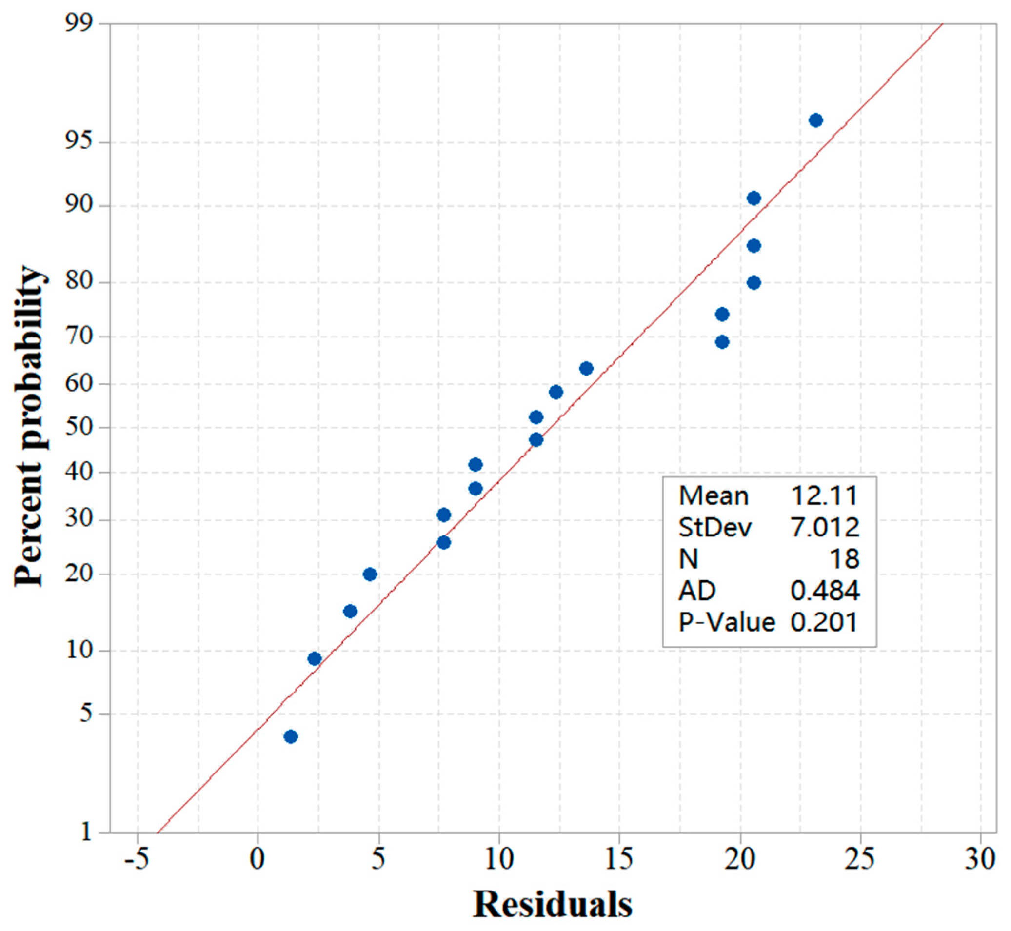
3.2. Anderson-Darling Normality Test Results

In the present work, the residuals are the difference between the experimental Δp and the predicted Δp by the established model (Equation (2)). The AD test was conducted by the software Minitab 17.0, and the probability distribution plot of the residuals is shown in the following Figure 3. As can be seen from the figure, the obtained AD value (0.484) is less than a critical value of 0.752, and the associated p-value (0.594) of the AD test is significant at a 5% level (p-value > 0.05) [25]. The results indicate that the residuals follow a normal distribution, and the deviation between the experimental Δp and predicted Δp are random [26]. Accordingly, it can be concluded that the null hypothesis can be rejected and the model predictions are correlated with the experimental data over the factor-space under evaluation in the present work.

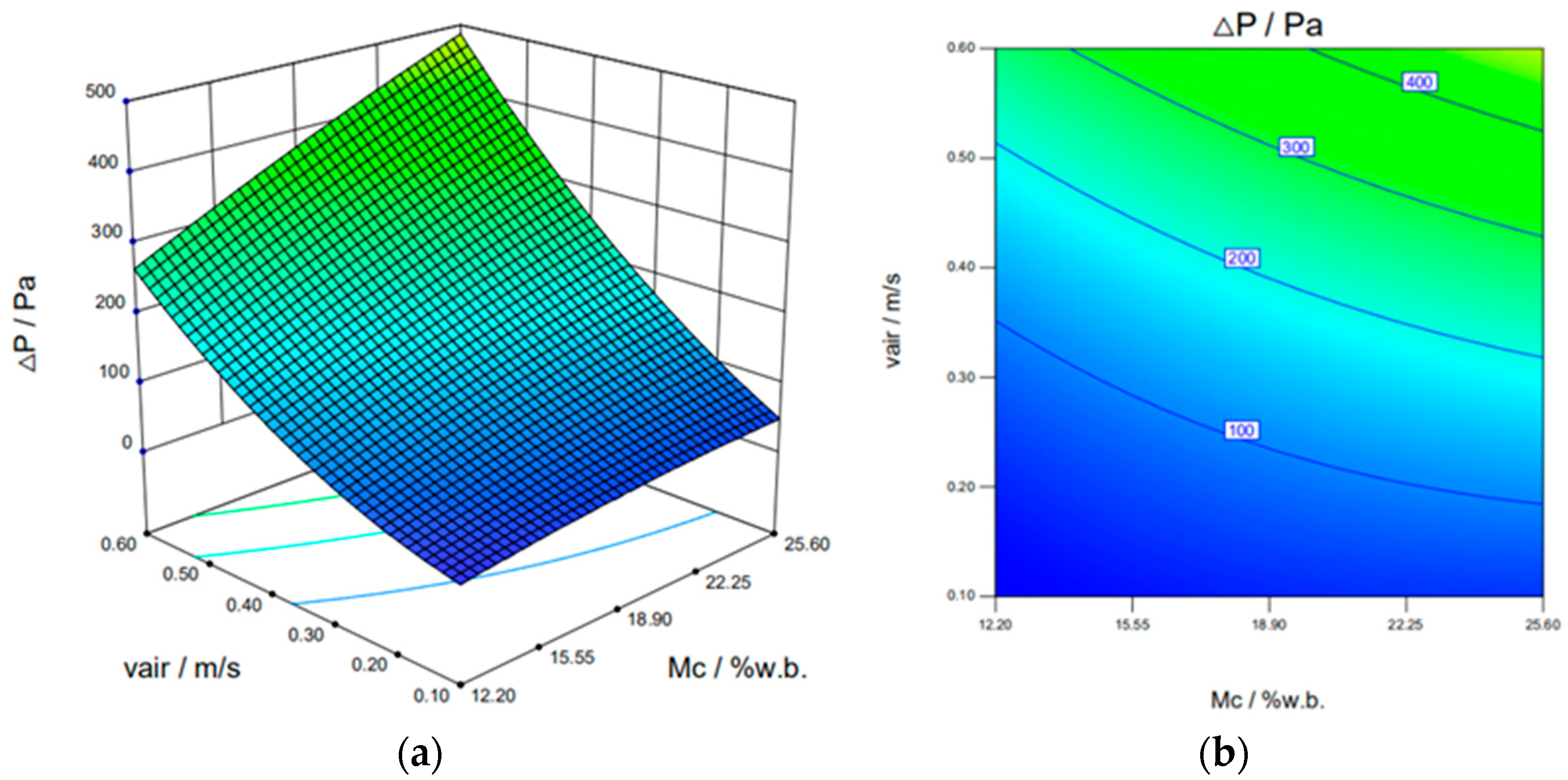
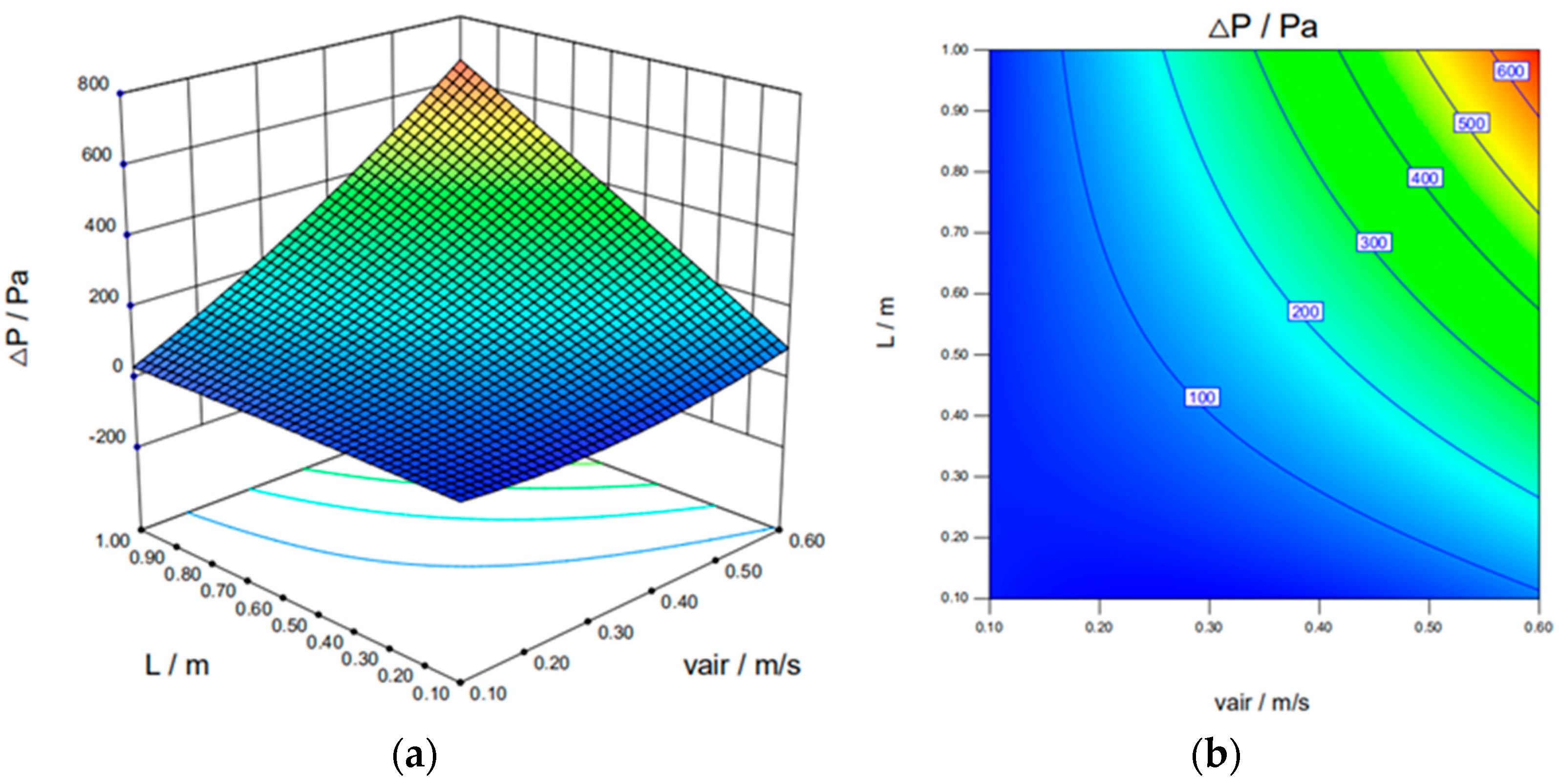
3.3. The Interactions of the Independent Variables on the Pressure Drop

Based on the ANOVA analysis in Section 3.1, the Mc·v_air, Mc·L, and v_air·L, respectively, have significant influences on the Δp. The response surface as well as its corresponding contour plots are depicted in the following Figure 4, Figure 5 and Figure 6. As can be seen from Figure 4a, the Δp increases with the increase of v_air under constant Mc, which might be due to the fact that the inertia resistance of the air increases with the increase of v_air, just as reported by Zhang et al. [10]. On the other hand, the Δp increases with increase of Mc under constant v_air, which might be caused by the increased ε in high Mc, just as reported by Li et al. that the ε of paddy layer increases with increase of paddy moisture content [38]. Though the suitable Δp for the engineering application should be further investigated by comprehensively considering the power of the fan, the contours shown in Figure 4b can be the reference for the single factor analysis.

Figure 5 depicts the interaction of Mc and L on the Δp, similar with the trend shown in above Figure 4. Δp increases with increase of L, which might be caused by the fact that the path of air flow through the paddy grain layer increases with the increase of L and further lead to the increase of Δp; a similar finding has been reported by Rocha et al. for Δp of paddy rice layer [39]. On the other hand, the Δp increases with increase of Mc; the same reason analyzed in Figure 4 can be also used to explain the trend. Interestingly, the Δp under different Mc with the L under 0.4 m almost remains constant, indicating that the Δp is slightly affected by the Mc when the L is small, which can be regarded as a design reference of the bed layer depth. Moreover, it can be seen from Figure 5a that the Δp linearly varies the single factor L or Mc, while the Δp non-linearly varies with the interaction terms of Mc·L, just as shown in the following Figure 5b.

The interaction of v_air and L on the Δp are shown in the following Figure 6. As can be seen from Figure 6a that the Δp varies from the minimum 17.11 Pa to the maximum 689.56 Pa, the variation range is much larger than that of the interaction terms of Mc·L and Mc·v_air, indicating that the influence of term L·v_air on Δp is more significant than that of Mc·L and Mc·v_air, just as analyzed in Section 3.1. Accordingly, in order to reach the objective of the efficient and energy-saving drying, efforts should be firstly made to optimize the drying parameters related to the L and v_air in the engineering drying application. Especially when the air with high v_air flow through the bed layer with large L, the Δp rapidly increases with the interaction term of L·v_air (as shown in Figure 6b, in other words, the larger driven force for supplying the drying medium is needed when the L·v_air is high.

3.4. The Comparison of the Δp Model Developed by RSM and Ergun Model

In order to verify the feasibility of the Δp model developed by RSM, the comparison analysis focused on the RSM experiments for the Δp model developed by RSM and Ergun model was conducted, and the statistical indexes including R², MAE, MSE, and RMSE were calculated. The detailed analysis is in Section 3.4.1.

3.4.1. The Comparison of the Δp in the RSM Experiments

Based on the ANOVA analysis results shown in Table 5, the second-order polynomial expression of the Δp model developed by the RSM (Δp_RSM) are expressed as following Equation (8):

$$\begin{array}{l}{\Delta p}_{\mathrm{RSM}}=174.60194-2.20717Mc-981.35993v_{air}-403.3567L+27.32537Mc·v_{air}\\ +15.95439Mc·L+1281.17778v_{air}·L-0.17375M{c}^2+645.768v_{air}^2-22.25679L^2\end{array}$$

(8)

The 17 sets of independent variables tabulated in Table 5 were substituted into the above Δp_RSM model and the predicted Δp_RSM values were obtained. On the other hand, the 17 sets of independent variables were also substituted into the Δp_Eur model shown in Equation (2) by transmitting the Mc into the corresponding ε (just as tabulated in Figure 2), and the predicted Δp_Eur values were obtained and compared with the corresponding predicted Δp_RSM. The comparison between the Δp_RSM and the Δp_Eur were evaluated by the validation metrics (Equations (2)–(5)), and the statistical results are tabulated in

Table 6. The statistical results of the RSM experiment for comparing Δp_RSM and Δp_Eur.

Statistical Indexes	RSM Model	Ergun Model
	Δ pRSM	Δ pEur
Determination coefficient (R2)	0.9948	0.9868
Mean-square error (MSE)	10.9021	15.7041
Mean absolute error (MAE)	2868.9372	7292.4115
Root-mean-square error(RMSE)	12.9908	20.7115

.

As can be seen from Table 6, the index R² (0.9948) of the RSM model is higher than that of the Ergun model (0.9868), while the indexes MAE, MSE, and RMSE of the RSM model are, respectively, lower than the corresponding index of the Ergun model, which indicates that the pressure drop model developed by the RSM is better fitted than the Ergun model.

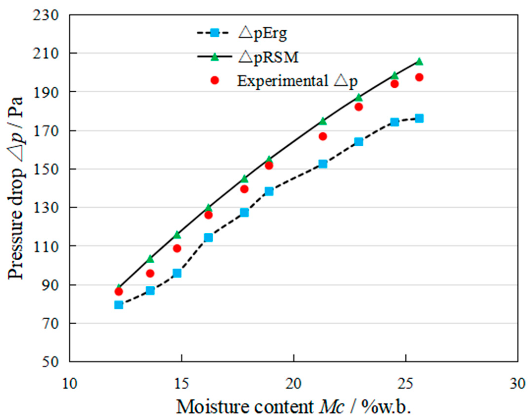
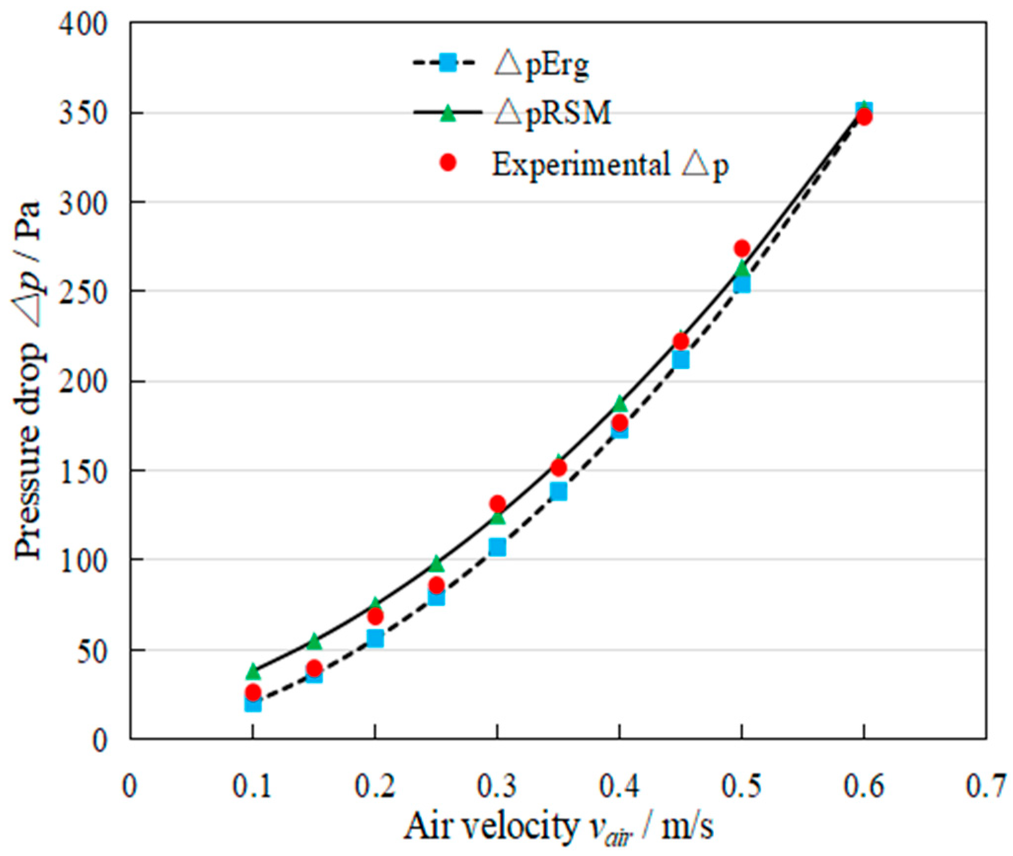
3.4.2. The Single Factor Analysis of the Δp

In order to validate fitting performance of the Δp_RSM and Δp_Erg. The second-order polynomial RSM model was transmitted into three first-order quadratic models by substituting the independent variables shown in Table 3 into Equation (8), the single factor pressure drop models based on the Δp_RSM are as follows:

$${\Delta p}_{Mc}=-72.8038915+19.7482445Mc-0.17375M{c}^2$$

(9)

$${\Delta p}_{{\mathrm{v}}_{air}}=14.4119253+175.678453{\mathrm{v}}_{\mathrm{air}}+645.768{\mathrm{v}}_{air}^2$$

(10)

$${\Delta p}_L=-12.72658565+346.593494L-22.25679L^2$$

(11)

Based on the above Equations (6), (9)–(11), the variations of Δp with Mc, v_air, and L can be obtained and, respectively, depicted in the following Figure 7, Figure 8 and Figure 9. As can be seen from Figure 7 that the Δp is proportional to the Mc, and the variation range of the Δp was ascertained to be 86.38–197.57 Pa. It can be summarized from Figure 2 that the equivalent diameter d_g increases with the Mc while porosity of the bed layer ε decreases with the increase of the Mc, indicating that the volume of the air pathways decreased with the increase of Mc [40], and further lead to the flow resistance of the air passing through the bed layer will be increased with the increase of the Mc. On the other hand, it can be seen from Figure 7 that the Δp_RSM are more closed to the experimental Δp than the Δp_Erg.

Figure 8 depicts the variations of Δp with v_air under the constant Mc of 18.9 %w.b. and L of 0.5 m. Similar with the variation trend of the Δp shown in the above Figure 7, Δp also increases with increase of v_air, and the variation range of the Δp was ascertained to be 38.44–352.92 Pa. Moreover, it can be seen from Figure 8 that the Δp_Erg with the v_air of 0.1 m/s and 0.15 m/s are more closed to the corresponding experimental Δp than the Δp_RSM, indicating that the Ergun model has a better prediction performance than the developed RSM model when the v_air is under 0.2 m/s. The same conclusions have been made by Mahmood et al. [41] and Ye et al. [10]. However, in this case, the developed Δp_RSM model has a better performance than the Ergun model when the v_air is above 0.2 m/s, which may be more suitable for guiding the actual process.

The variations of Δp with L under the constant v_air of 0.35 m/s and Mc of 18.9 %w.b. are depicted in Figure 9. It can be seen from the figure that the Δp linearly increases with the increase of L, and the Δp gets the minimum (27.68 Pa) and maximum value (276.83 Pa), respectively, at the L of 0.1 and 1m. On the other hand, it can be also seen from Figure 9 that, for the all levels of L, the fitting performance of the Δp_RSM is better than that of the Δp_Erg. In order to further investigate the fitting performance of the Δp_RSM and the Δp_Erg in the above three single factor experiment, the statistical indexes mentioned in Section 2.3.3 were also calculated and the results are tabulated in the following

Table 7. The statistical results for the single factor experiments.

Statistical Indexes	RSM Model			Ergun Model
	ΔpMc	Δpvair	ΔpL	ΔpMc	Δpvair	ΔpL
Determination coefficient (R2)	0.9755	0.9909	0.9918	0.8539	0.9846	0.9737
Mean-square error (MSE)	35.9195	89.4276	64.5378	213.7543	151.9289	206.1363
Mean absolute error (MAE)	5.6094	8.4528	6.3943	13.9521	10.1731	12.6444
Root-mean-square error(RMSE)	5.9933	9.4566	8.0335	14.6203	12.3259	14.3574

.

As can be seen from Table 7 that the R² value of each single factor model based on the Δp_RSM is higher than that of the corresponding model based on the Δp_Erg, while the other indexes (MSE, MAE, and RMSE) of each single factor model based on the Δp_RSM are lower than the corresponding index of the corresponding model based on the Δp_Erg. Which indicates that the single factor model Δp_Mc, Δp_vair, and Δp_L based on the Δp_RSM has better fitting performance than that of the corresponding single factor model based on the Δp_Erg. By combining the results obtained in Section 3.4.1, it can be concluded that the developed ventilation resistance model based on the RSM has a better predicting performance than the traditional Ergun model.

4. Conclusions

By considering the moisture content (Mc), air velocity (v_air), and grain bed layer depth (L) as the key factors affecting the ventilation resistance of the air, one must regard the pressure drop (Δp) as the key index characterizing the ventilation resistance of the air. The present work investigated the influences of each factor and the interactions of the factors on the pressure drop; a second-order polynomial model was also obtained based on the RSM. The detailed conclusions depending on the main results are listed as follows:

(1)

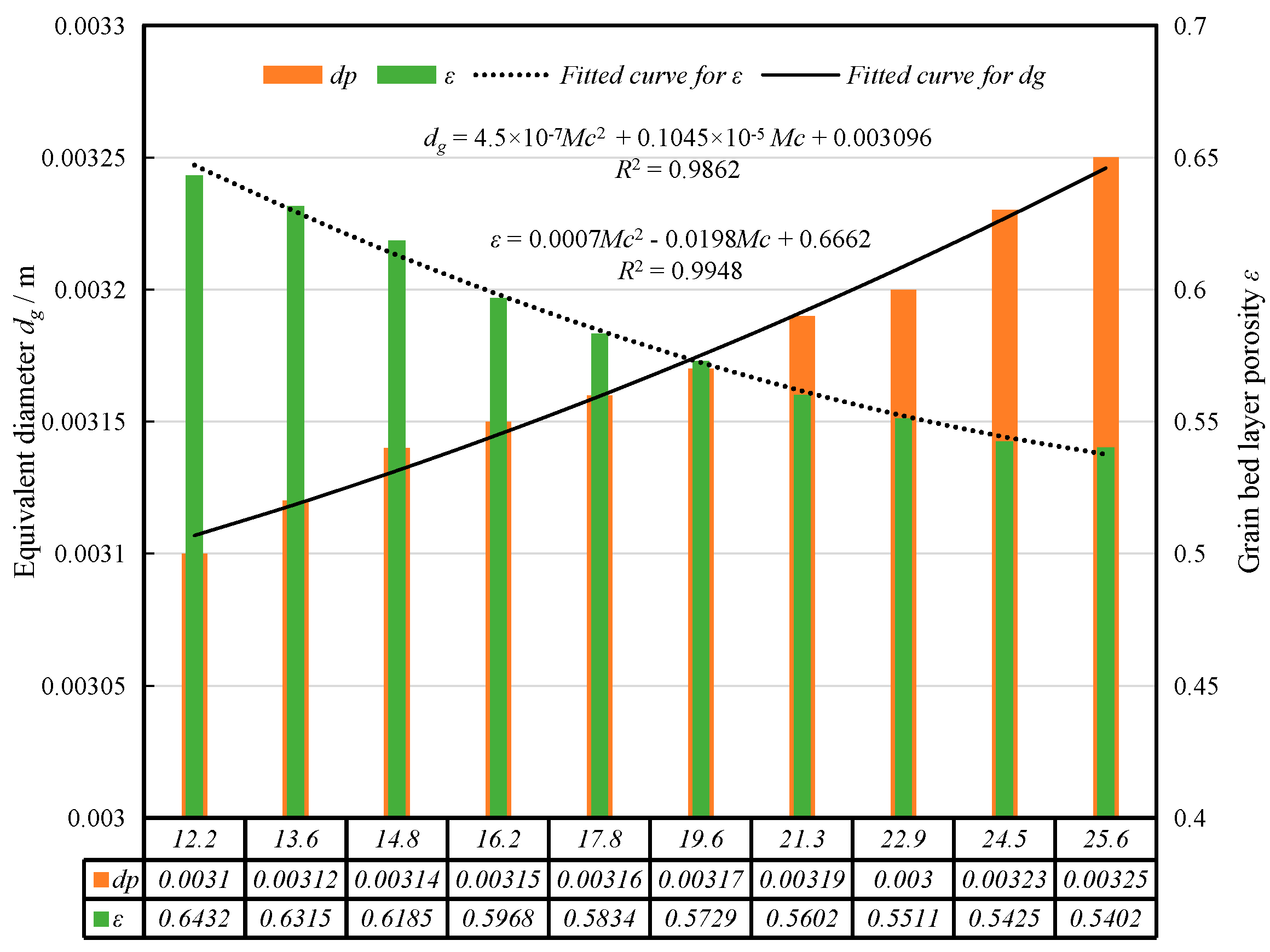
The relations among the Mc, ε, and d_g were revealed and the mathematical expressions were also given in the present work.

(2)

The Δp increases with the increase of Mc, v_air, and L and the contributors to the Δp, in ascending order of significance, are as follows: Mc < L < v_air.

(3)

The interaction analysis indicates that the interactions of the v_air and L has the most significant influence on the Δp, and the match principle between the v_air and L should be firstly considered when optimizing the drying process.

(4)

A second-order polynomial Δp model based on the RSM was obtained, and its fitting performance was verified to be better than that of the traditional Ergun model by evaluating the R², MSE, MAE, and RMSE.

(5)

The developed Δp model based on the RSM shows a better fitting performance than the Ergun model when the v_air ≥ 0.2 m/s, while the Ergun model shows better when the v_air is under 0.2 m/s.

The present work revealed the influences of the variables that can be directly measured in an engineering drying application on the pressure drop and established a prediction model of the pressure drop. Thus, the main results would be helpful for further optimizing the drying process. Further study is recommended to investigate the pressure drop variation characteristics by taking the air temperature as well as the paddy grain flow velocity into consideration.

References

1. Mujumdar, A.S. Handbook of Industrial Drying, 3rd ed.; Taylor & Francis Group: Abingdon, UK; CRC Press: Boca Raton, FL, USA, 2006. [Google Scholar] [CrossRef]
2. Li, C. Theoretical analysis of exergy transfer and conversion in grain drying process. Trans. Chin. Soc. Agric. Eng. 2018, 34, 1–8. [Google Scholar] [CrossRef]
3. Li, J.; Li, C.; Ma, X. Experimental study on ventilation resistance of paddy. Guangdong Agric. Sci. 2012, 39, 191–193. [Google Scholar] [CrossRef]
4. Chu, J.C.; Teng, J.T.; Xu, T.T.; Huang, S.; Jin, S.; Yu, X.F. Characterization of frictional pressure drop of liquid flow through curved rectangular microchannels. Exp. Therm. Fluid Sci. 2012, 38, 171–183. [Google Scholar] [CrossRef]
5. Norouzi, A.M.; Siavashi, M.; Soheili, A.R.; Oskouei, M.H.K. Experimental investigation of effects of grain size, inlet pressure and flow rate of air and argon on pressure drop through a packed bed of granular activated carbon. Int. Commun. Heat Mass Transf. 2018, 96, 20–26. [Google Scholar] [CrossRef]
6. Spieler, O.; Alidibirov, M.; Dingwell, D.B. Grain-size characteristics of experimental pyroclasts of 1980 mount st. helens cryptodome dacite: Effects of pressure drop and temperature. Bull. Volcanol. 2003, 65, 90–104. [Google Scholar] [CrossRef]
7. Yue, R.; Zhang, Q. A pore-scale model for predicting resistance to airflow in bulk grain. Biosyst. Eng. 2017, 155, 142–151. [Google Scholar] [CrossRef]
8. Gunasekaran, S.; Jackson, C.Y. Resistance to airflow of grain sorghum. Trans. ASAE 1988, 31, 1237–1240. [Google Scholar] [CrossRef]
9. Li, Q.T.; Hu, T.Q.; Yu, Z.; Yang, Y.Q.; Fang, Y.L. Experimental study of fluid drag in granary ventilation. J. Hydrodyn. (Ser. A) 2006, 21, 473–478. [Google Scholar]
10. Zhang, Y.; Li, C.; Ma, X.; Li, J.; Zou, X.; Wang, R. Experiment and Numerical Simulation of Layer Resistance Parameters in Dryer. Trans. Chin. Soc. Agric. Mach. 2014, 45, 216–221. [Google Scholar] [CrossRef]
11. Li, B.; Peng, G.; Luo, C.; Qiu, G.; Yang, L. Optimization of rapeseed vacuum drying technology parameter by response surface methodology. Food Ferment. Ind. 2016, 42, 105–110. [Google Scholar] [CrossRef]
12. Wang, X.; Wu, Y.; Chen, G.; Yue, W.; Liang, Q.; Wu, Q. Optimisation of ultrasound assisted extraction of phenolic compounds from sparganii rhizoma with response surface methodology. Ultrason. Sonochem. 2013, 20, 846–854. [Google Scholar] [CrossRef]
13. Zeng, Z.; Chen, M.; Wang, X.; Wu, W.; Zheng, Z.; Hu, Z.; Ma, B. Modeling and Optimization for Konjac Vacuum Drying Based on Response Surface Methodology (RSM) and Artificial Neural Network (ANN). Processes 2020, 8, 1430. [Google Scholar] [CrossRef]
14. Liu, S.; Zhang, H.; Wang, J.; Zhang, C.; Sun, L.; Qi, W. Optimization design of fertilizer-guiding mechanism for orchard ditching and fertilizing machin. J. Chin. Agric. Mech. 2017, 38, 45–53. [Google Scholar] [CrossRef]
15. Kowalczyk, P.; Ligas, B.; Skrzypczak, D.; Mikula, K.; Chojnacka, K. Biosorption as a method of biowaste valorization to feed additives: Rsm optimization. Environ. Pollut. 2020, 268, 115937. [Google Scholar] [CrossRef] [PubMed]
16. Sander, A.; Kardum, J.P.; Skansi, D. Transport properties in drying of solids. Chem. Biochem. Eng. Q. 2000, 15, 131–137. [Google Scholar] [CrossRef]
17. Brzinski, T.A., III; Mayor, P.; Durian, D.J. Depth-dependent resistance of granular media to vertical penetration. Phys. Rev. Lett. 2013, 111, 168002. [Google Scholar] [CrossRef] [Green Version]
18. Yang, Z.; Luo, X.; Li, C. Study on optimal ratio of air flux to grain mass for rough rice drying. Trans. Chin. Soc. Agric. Mach. 2007, 38, 122–125. [Google Scholar] [CrossRef]
19. Jiang, H.; Yang, L.; Xing, X.; Yan, M.; Guo, X.; Yang, B.; Wang, Q.; Kuang, H. Chemometrics coupled with UPLC-MS/MS for simultaneous analysis of markers in the raw and processed Fructus Xanthii, and application to optimization of processing method by BBD design. Phytomedicine 2018, 57, 191–202. [Google Scholar] [CrossRef] [PubMed]
20. Gupta, M.K.; Sehgal, V.K.; Arora, S. Optimization of drying process parameters for cauliflower drying. J. Food Sci. Technol. 2013, 5, 62–69. [Google Scholar] [CrossRef] [PubMed] [Green Version]
21. Mhe, A.; Mhh, A.; Shr, B. Multi-objective particle swarm optimization of thermal conductivity and dynamic viscosity of magnetic nanodiamond-cobalt oxide dispersed in ethylene glycolusing RSM. Int. Commun. Heat Mass Transf. 2020, 117, 104760. [Google Scholar] [CrossRef]
22. Aflaki, S.; Memarzadeh, M. Using two-way anova and hypothesis test in evaluating crumb rubber modification (crm) agitation effects on theological properties of bitumen. Constr. Build. Mater. 2011, 25, 2094–2106. [Google Scholar] [CrossRef]
23. Cdd, A.; Yntn, A.; Dlt, B.; Quan, N.; Dcnb, C.; Long, G. Extraction conditions of polyphenol, flavonoid compounds with antioxidant activity from veronia amygdalina del. leaves: Modeling and optimization of the process using the response surface methodology rsm. Mater. Today: Proc. 2019, 18, 4004–4010. [Google Scholar] [CrossRef]
24. Chokphoemphun, S.; Chokphoemphun, S. Moisture content prediction of paddy drying in a fluidized-bed drier with a vortex flow generator using an artificial neural network. Appl. Therm. Eng. 2018, 145, 630–636. [Google Scholar] [CrossRef]
25. Konwarh, R.; Misra, M.; Mohanty, A.K.; Karak, N. Diameter-tuning of electrospun cellulose acetate fibers: A Box–Behnken design (BBD) study. Carbohydr. Polym. 2013, 92, 1100–1106. [Google Scholar] [CrossRef] [PubMed]
26. Myer, R.H.; Montogomery, D.C. Response Surface Methodology: Process and Product Optimization Using Designed Experiment, 2nd ed.; John Wiley & Sons: New York, NY, USA, 2002; pp. 343–350. [Google Scholar]
27. Box, G.E.P.; Draper, N.R. Empirical Model Building and Response Surfaces; John Wiley & Sons: New York, NY, USA, 1987; pp. 205–477. [Google Scholar]
28. Huang, W.; Luo, Z.; Zhuang, H. Pressure drop calculation model of air dense-medium fluidized bed. Coal Eng. 2014, 46, 117–119. [Google Scholar] [CrossRef]
29. Vicente, P.G.; Garcia, A.; Viedma, A. Mixed convection heat transfer and isothermal pressure drop in corrugated tubes for laminar and transition flow. Int. Commun. Heat Mass Transf. 2004, 31, 651–662. [Google Scholar] [CrossRef]
30. Sieder, E.N.; Tate, G.E. Heat transfer and pressure drop of liquids in tubes. Ind. Eng. Chem. 1936, 28, 1429–1435. [Google Scholar] [CrossRef]
31. Sarker, M.S.H.; Ibrahim, M.N.; Aziz, N.A. Energy and rice quality aspects during drying of freshly harvested paddy with industrial inclined bed dryer. Energy Convers. Manag. 2014, 77, 389–395. [Google Scholar] [CrossRef]
32. Li, B.; Li, C.; Li, T.; Zeng, Z.; Ou, W.; Li, C. Exergetic, Energetic, and Quality Performance Evaluation of Paddy Drying in a Novel Industrial Multi-Field Synergistic Dryer. Energies 2019, 12, 4588. [Google Scholar] [CrossRef] [Green Version]
33. Li, C.; Fang, Z.; Mai, Z. Design and Test on Porosimeter for Particle Material. Trans. Chin. Soc. Agric. Mach. 2014, 45, 200–206. [Google Scholar] [CrossRef]
34. Li, T.; Li, C.; Li, C.; Xu, F.; Fang, Z. Porosity of flowing rice layer: Experiments and numerical simulation. Biosyst. Eng. 2019, 179, 1–12. [Google Scholar] [CrossRef]
35. Aghbashlo, M.; Mandegari, M.; Tabatabaei, M.; Farzad, S.; Soufiyan, M.M.; Görgens, J.F. Exergy analysis of a lignocellulosic-based biorefinery annexed to a sugarcane mill for simultaneous lactic acid and electricity production. Energy 2018, 149, 623–638. [Google Scholar] [CrossRef]
36. Erbay, Z.; Icier, F. Optimization of hot air drying of olive leaves using response surface methodology. J. Food Eng. 2009, 91, 533–541. [Google Scholar] [CrossRef]
37. Dalvand, M.J.; Mohtasebi, S.S.; Rafiee, S. Modeling of electrohydrodynamic drying process using response surface methodology. Food Sci. Nutr. 2014, 2, 200–209. [Google Scholar] [CrossRef] [PubMed]
38. Li, C.; Mai, Z.; Fang, Z. Analytical study of grain moisture binding energy and hot air drying dynamics. Trans. Chin. Soc. Agric. Eng. 2014, 30, 236–242. [Google Scholar] [CrossRef]
39. Rocha, J.C.D.; Pohndorf, R.S.; Meneghetti, V.L.; de Oliveira, M.; Elias, M.C. Effects of mass compaction on airflow resistance through paddy rice grains. Biosyst. Eng. 2020, 194, 39. [Google Scholar] [CrossRef]
40. Yang, Y.Q.; Yu, Z. Experimental Study of Grain Physics and Grain Bulk Resistance. Res. Explor. Lab. 2008, 27, 32–34. [Google Scholar] [CrossRef]
41. Bazmi, M.; Hashemabadi, S.H.; Bayat, M. Modification of ergun equation for application in trickle bed reactors randomly packed with trilobe particles using computational fluid dynamics technique. Korean J. Chem. Eng. 2011, 28, 1340–1346. [Google Scholar] [CrossRef]
Figure 1. The schematic diagram of the laboratory-scale experimental apparatus.
Applsci 11 07826 g001
Figure 2. The variations of the dg and ε with Mc.
Applsci 11 07826 g002
Figure 3. The results of the Anderson–Darling normality test.
Applsci 11 07826 g003
Figure 4. The interaction of Mc and vair on the Δp (a) and the contour plots (b).
Applsci 11 07826 g004
Figure 5. The interaction of Mc and L on the Δp (a) and the contour plots (b).
Applsci 11 07826 g005
Figure 6. The interaction of vair and L on the Δp (a) and the contour plots (b).
Applsci 11 07826 g006
Figure 7. The variations of Δp with Mc under the constant vair of 0.35 m/s and L of 0.5 m.
Applsci 11 07826 g007
Figure 8. The variations of Δp with vair under the constant Mc of 18.9 %w.b. and L of 0.5 m.
Applsci 11 07826 g008
Figure 9. The variations of Δp with L under the constant vair of 0.35 m/s and Mc of 18.9 %w.b.
Applsci 11 07826 g009