Classification of Imbalanced Data Represented as Binary Features

Abstract

Typically, classification is conducted on a dataset that consists of numerical features and target classes. For instance, a grayscale image, which is usually represented as a matrix of integers varying from 0 to 255, enables one to apply various classification algorithms to image classification tasks. However, datasets represented as binary features cannot use many standard machine learning algorithms optimally, yet their amount is not negligible. On the other hand, oversampling algorithms such as synthetic minority oversampling technique (SMOTE) and its variants are often used if the dataset for classification is imbalanced. However, since SMOTE and its variants synthesize new minority samples based on the original samples, the diversity of the samples synthesized from binary features is highly limited due to the poor representation of original features. To solve this problem, a preprocessing approach is studied. By converting binary features into numerical ones using feature extraction methods, succeeding oversampling methods can fully display their potential in improving the classifiers’ performances. Through comprehensive experiments using benchmark datasets and real medical datasets, it was observed that a converted dataset consisting of numerical features is better for oversampling methods (maximum improvements of accuracy and F1-score were 35.11% and 42.17%, respectively). In addition, it is confirmed that feature extraction and oversampling synergistically contribute to the improvement of classification performance.

1. Introduction

In the field of machine learning, it is important to understand the characteristics of input data and select the methods that are most suitable for achieving high performance in the machine learning task (regression, classification, clustering, etc.).

Class imbalance is a common issue arising from real-world data, such as in the field of marketing [1], medical diagnosis [2,3], and finance [4]. This problem occurs when the number of data represented in a class is smaller than in the other(s) class(es), as in a rare disease dataset. Typically, the minority class is more important and becomes the target class in classification. Therefore, the class imbalance issue is more sensitive to classification errors for the minority class than the majority class. This issue is an obstacle for classifiers to accurately predict the minority class, because the classifier will be more likely to predict minority class data than majority class data. Numerous approaches have been introduced to deal with class imbalance. The methods vary at either data level or algorithm level. At the data level, resampling is a widely method adopted to balance the class distribution. This method includes undersampling the majority class and oversampling the minority class. The most well-known data-level approach for oversampling imbalanced data is the synthetic minority oversampling technique (SMOTE) [5], which creates synthetics samples using k-nearest neighbor to balance the dataset instead of replicating the minority data.

After [5] introduced this technique, some approaches started to be developed based on SMOTE and focused on overcoming its drawback(s) [6,7,8,9,10,11,12,13,14,15,16]. Despite the fact that opinions about the best resampling method for the class imbalance problem vary, numerous studies have found that oversampling generally outperforms undersampling in dealing with the class imbalance problem [17,18,19]. At the algorithm level, a method is proposed to modify the algorithm by either changing or adding another line of algorithm to solve this problem. Ensemble learning such as AdaC2 [20] and cost-sensitive learning such as cost-sensitive decision tree [21] are some examples of algorithm-level methods.

However, many of the available methods were specifically developed to overcome this problem in numerical datasets or mixed datasets of numerical and categorical data. In contrast, some types of data are represented as binary values that can only take one of two values (0/1, T/F, M/F, etc.). Such binary features are located on the border of numerical and categorical values. They can be treated as numerical values; however, the domain of value is quite poor and presents no difference from a categorical value. Therefore, for a dataset consisting of binary features, direct application of oversampling methods is not a good idea, since such methods rely on numerically represented values for synthesizing new minority samples.

In this paper, we investigated an approach using feature extraction for converting binary features into numerical features prior to oversampling. Though it is popular to combine an oversampling algorithm with a feature extraction algorithm such as principal component analysis (PCA), the purpose of this combination is usually dimension reduction [22], and the positive effect of feature extraction from binary features followed by oversampling has not been analyzed in detail.

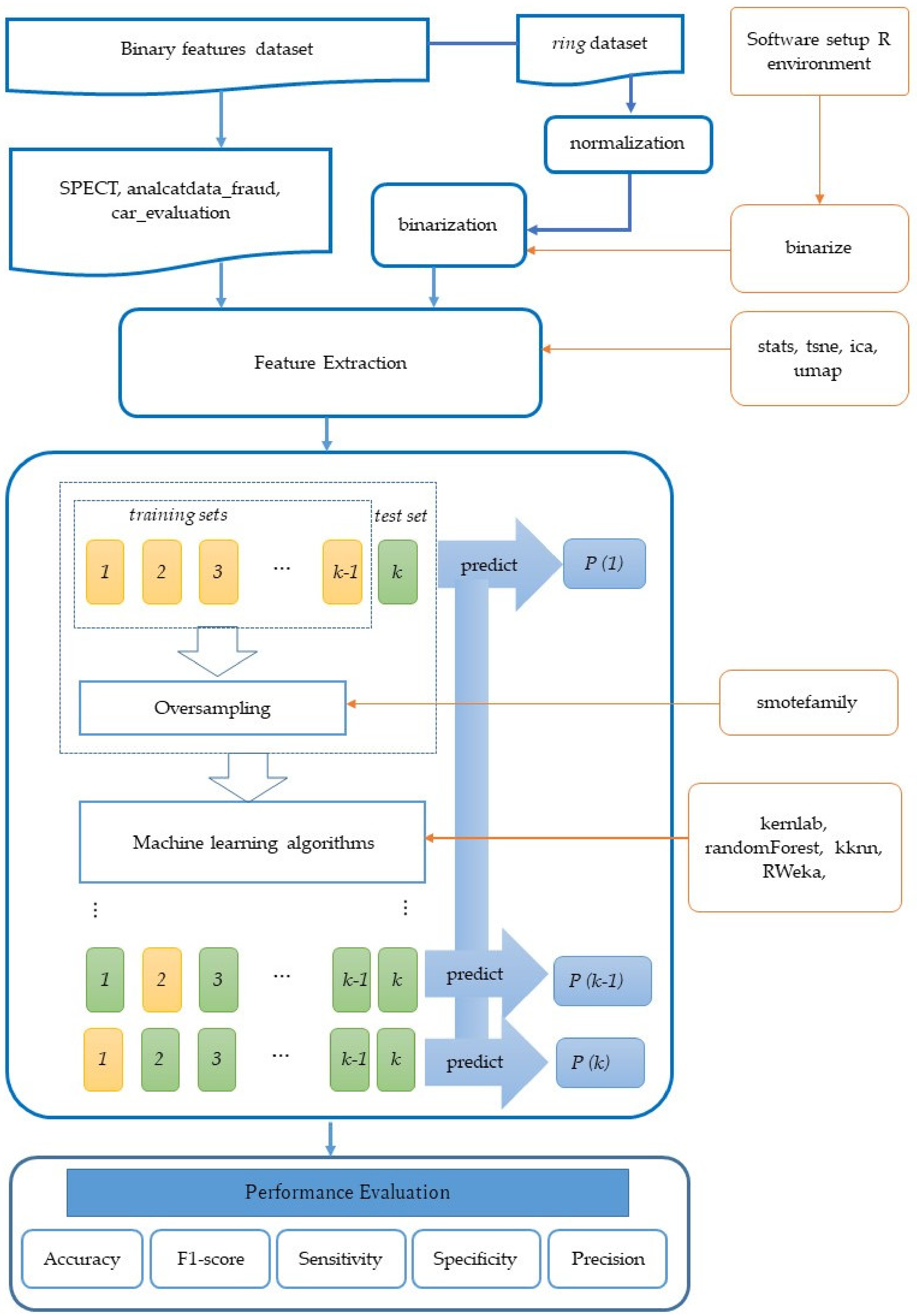
The flowchart of our approach is shown in Figure 1. Using various datasets, classifiers, feature extraction methods, and oversampling methods, classification performances were measured. Through comprehensive experiments, the effectiveness of the approach was confirmed.

2. Materials and Methods

2.1. Data Description

All the datasets used in this study are binary feature datasets, which means all of the input data were binary (values of target class can be also represented as binary, but they are treated as categorical values). To enable the performance evaluation from various viewpoints, we selected public datasets with binary features (SPECT, analcatdata_fraud), a public dataset with binary features for multiclass classification (car_evaluation), biomedical datasets with large number of binary features (Methicillin-resistant Staphylococcus Aureus (MRSA) pathogenicity, MRSA drug resistance, C. difficile pathogenicity), and a public dataset for generating a various number of samples and target class ratios through the artificial binarization of numerical features (ring).

Three of the datasets, SPECT, analcatdata_fraud, and ring, are benchmark datasets retrieved from GitHub repository of [23]. SPECT and analcatdata_fraud are datasets for which all the input data are binary. The ring dataset’s input data were originally numerical with two class labels (binary), which then were normalized and binarized using the k-means clustering algorithm of the “Binarize” R package. This was done to generate datasets with various degree of imbalance. ring_1500vs3000, ring_100vs500, ring_100vs2000, and ring_60vs3000 were randomly generated from the ring dataset. The same procedure was also performed by [24] in order to evaluate their models based on different degrees of imbalance due to the lack of available datasets.

The other three datasets are biological datasets obtained at Kanazawa University Hospital. Two datasets about MRSA share basically the same feature data, which represent the existence of mutations in each strain of MRSA corresponding to each sample [25]. The main difference in the two MRSA datasets is the target class. In the MRSA pathogenicity dataset, 0 and 1 represent latent and developed, respectively. In the MRSA drug resistance dataset, the target class represents the resistance of each strain to Clindamycin (CLDM). Similarly, the C. difficile pathogenicity dataset contains feature data representing the existence of mutations in each strain of C. difficile, which causes diarrhea in humans and poses difficulties in antibiotic treatment. To generate the feature data, the whole genomes of 77 strains were sequenced by Hiseq 2500 with 150 base reads. The reads were mapped to the reference genome NC_009089 in RefSeq (the same as AM180355.1 in GenBank) by BWA. After the mapping and file conversion by SAMtools, mutations were detected by Varscan. Among the two types of mutation, Indels and SNPs, we only used Indels (insertions and deletions). After the detection of Indels, if the feature data (existence of mutation) of two or more Indels were completely the same in 77 strains, the features were integrated as one, since such redundant features often have a harmful influence on the performance of classification by machine learning. Finally, 2610 features were generated for 77 samples, where each feature corresponded to one or more mutation. For the multiclass case, due to the difficulty in finding a benchmark dataset that met our criteria, we only used one dataset to show that our approach can also be applied to multiclass binary features datasets.

The number of samples and other basic information of the datasets are summarized in

Table 1. Basic information of the dataset used in this study.

Dataset	Number of Features	Number of Samples	Target Class Ratio
SPECT	22	267	55:212
analcatdata_fraud	10	42	29:13
car_evaluation	22	1728	1210:384:65:69
MRSA pathogenicity	1978	96	33:63
MRSA drug resistance	1976	94	75:19
C. difficile pathogenicity	2610	77	46:31
ring_1500vs3000	20	4500	1500:3000
ring_100vs500	20	600	100:500
ring_100vs2000	20	2100	100:2000
ring_60vs3000	20	3060	60:3000

. All the input variables of these datasets are binary, and all the target class were also binary, except for the car_evaluation dataset, which has four classes for the target class. All the features of these datasets were used in the analysis.

2.2. Oversampling Methods

Imbalanced datasets exist in many real-world data. Class imbalance occurs when the number of samples in a class is far less than in the other class(es). The target class is usually the minority class or the class which has far fewer samples than the other class(es), and a sample in this class is called as positive sample, while a sample from the other class is called as negative sample. This problem can lead classifiers to bias toward the majority class, because it will be most likely to predict a positive sample as a negative sample. Therefore, a method to deal with class imbalance should be performed first before providing the data as an input to the classifiers to improve the detection of minority samples and the performance metrics. Many methods exist to deal with class imbalance either at the algorithm level or the data level. At the algorithm level, methods have been proposed to modify the algorithm by either changing or adding another line of algorithm to solve the imbalanced data problem.

At the data level, there are multiple available forms of the resampling method. This method consists of oversampling and undersampling to rebalance the original dataset. The undersampling method is performed by removing samples of the majority class, while oversampling method is performed by adding samples of the minority class to the original dataset so that the new dataset becomes balanced.

The synthetic minority oversampling technique (SMOTE) is known as the pioneer method for rebalancing an imbalanced dataset. The method uses k-nearest neighbors in creating new synthetic samples to balance the class distribution of the dataset [5]. Each positive sample is paired with its nearest neighbors, and then, along a line connecting the sample with one of the selected nearest neighbors, a synthetic sample is generated. The process is repeated until the number of positive and negative samples becomes balanced. Many methods were developed to improve the classification performances based on SMOTE technique.

ADASYN, or the adaptive synthetic sampling approach for imbalance learning, is another technique to deal with class imbalance. The main idea of this method is to create synthetic samples based on the level of difficulty in learning the samples of the minority class [6]. A positive sample is labelled as difficult to learn if it has more negative samples in its k-nearest neighbors. Therefore, the harder a positive sample is to learn, the more synthetic samples are generated.

Borderline SMOTE is a SMOTE-based technique concentrating on the borderline of each class [7]. It states that a sample located on or near the borderline will provide a greater contribution to classification. It highlights the problem that borderline samples tend to be misclassified by classification methods for often than samples located far from the borderline. For that reason, this technique tries to strengthen the borderline of positive samples by generating synthetic samples along this region. This idea of borderline SMOTE in selecting certain regions to generate synthetic samples inspired other SMOTE-based techniques in oversampling methods, such as safe-level SMOTE and relocating safe level SMOTE.

Another improvement of SMOTE, namely safe-level SMOTE [8], highlighted the drawbacks of SMOTE, in that SMOTE naively ignores nearby majority instances in synthesizing the minority samples along a joining line of a minority sample and its selected nearest neighbors. This newly generated synthetic sample by SMOTE causes classifiers to create larger and less specific regions, which results in overgeneralization. Therefore, safe-level SMOTE will determine whether a sample in a minority class is safe to use in generating synthetic samples or not. In other words, safe-level SMOTE is designed to generate synthetic samples around the selected positive samples that are considered as safe.

Relocating-safe-level SMOTE (RSLS) is as an improvement on safe-level SMOTE [9]. It highlights the fact that safe-level SMOTE ignores the possibility that some synthetic samples are generated closer to negative samples than to positive samples. It contradicts the procedure of generating synthetic samples in safe-level SMOTE, as it tries to avoid negative samples when generating synthetic samples. Therefore, RSLS introduced an additional algorithm to relocate the generated synthetic samples if they are generated near to negative samples.

Another variation of SMOTE-based oversampling techniques is the density-based minority oversampling technique, or DBSMOTE. It is an integration of DBSCAN and SMOTE [10]. DBSCAN, or density-based spatial clustering of application with noise, aims at discovering clusters with an arbitrary shape [26]. DBSMOTE aims at generating synthetic samples of an arbitrarily shaped cluster found using DBSCAN. Inspired by borderline-SMOTE in maintaining the detection rate of majority class, DBSMOTE focuses the work on the overlapping region. However, this technique also highlights the drawbacks of borderline SMOTE, which fails in maintaining the detection rate of positive samples while improving the detection rate of negative samples. To resolve this drawback, DBSMOTE developed a different approach towards precise oversampling, both in the overlapping and the safe region, by synthesizing a minority instance along the shortest path retrieved in a directly density-reachable graph from each sample to the pseudo-centroid cluster.

While the methods mentioned above focus on where to generate synthetic samples, Adaptive Neighbor SMOTE (ANS) focuses on the number of neighbors needed to ideally synthesize a new sample [11]. In other words, ANS concentrates on deciding the appropriate value for the parameter k in k-nearest neighbors of each positive sample that is needed in synthesizing a new sample. The parameter k is selected according to the density level of each positive sample’s region. By utilizing the value of k, the area of the generated synthetic samples will be more spread out inside the dense area and not sparsely distributed, as in SMOTE.

2.3. Feature Extraction Methods

Feature extraction is a process meant to create new variables from the existing variables without losing the information of the original dataset. This process is conducted for various purposes, such as to reduce the problem arising from highly dimensional datasets, to increase computational efficiency, or to visualize the dataset either in 2D or 3D.

PCA is a linear feature extraction method that is commonly used to reduce the dimensions of a highly dimensional dataset. PCA orthogonally transforms the dimensions of a large set of variables into a smaller set of variables known as principal components to identify the correlation and pattern of the original dataset [27]. In this technique, a considered non-significant principal component is excluded, which results in a less dimensional projection while preserving the maximal variance of the dataset. By reducing dimensionality of original dataset, PCA provides an efficient method for data description, visualization, and classification.

Another linear method of feature extraction using component analysis is independent component analysis (ICA). ICA is an important method in signal-based analysis, such as EEG signals, to help separate normal and abnormal signals. ICA aims to extract the hidden factors of a dataset by transforming the variables to a new set of variables that is maximally independent [28]. What distinguishes ICA from PCA is that PCA assumes that signals are subject to multivariate Gaussian distribution and uses orthogonal bases to decompose signals. It can be concluded that ICA’s goal is to find the linear transformation of a highly dimensional dataset in which the basis vectors are non-Gaussian and statistically independent, while PCA’s goal is to find an orthogonal transformation that maximizes the variable’s variance of the dataset.

Other than linear dimensionality reduction techniques, there are some available techniques that are nonlinear. One familiar use of these techniques is t-distributed stochastic neighbor embedding (t-SNE), which reduces the dimensionality of a dataset by giving each data point a location in a 2D or 3D dimensional map. This technique aims at identifying the relevant pattern of a dataset while maintaining its local structure [29]. For each point of a dataset, t-SNE models the probability distribution of other points which are closest to it. One of the most important parameters to be set when using t-SNE is perplexity, which is the expected number of nearest neighbors each point has. The performance of t-SNE is fairly robust under different settings of this parameter. Generally, the perplexity is set depending on the size of the dataset. The default value of perplexity in some packages is set to 30 for a dataset whose variables are more than 30.

Uniform manifold approximation and projection for dimension reduction (UMAP) is another nonlinear dimensionality reduction technique which builds a mathematical theory to justify the graph-based approach [30]. It was developed based on ideas from topological data analysis and manifold learning techniques, which assume that the data are uniformly distributed on the manifold. To make this assumption true, it defines a Riemannian metric on the manifold. Compared to t-SNE, UMAP provides much faster computational running time.

2.4. Classification Methods

2.4.1. K-Nearest Neighbor

K-nearest neighbor (k-NN) is a simple classification algorithm which does not require any training. From a statistics perspective, k-NN is a nonparametric classification method, which means that it needs no underlying assumptions about the data or its distribution pattern in general. In the two-class classification, the value of k is usually set to an odd positive integer, because if it is set to be an even number, there is a possibility that the number of positive and negative samples in the k-nearest neighbor is equal. This can lead to a tie in the decision; that is, two class labels achieving the same score because the k-NN algorithm takes the majority as the class label for the given test sample.

In the imbalanced data case, samples of minority classes appear sparsely in the data space when there are uneven training data. The calculated k-nearest neighbors bear higher probabilities of samples from the prevalent classes when given a test sample. As a result, given test data from minority classes are more likely to be classified wrongly. However, k-NN can be used in combination with sampling techniques such as oversampling or undersampling to improve the classifier’s performance [31]. They reported that for the performance metric of sensitivity, k-NN gave a higher result than SVM and logistic regression (LR) when combined with oversampling techniques.

2.4.2. Decision Tree C4.5

C4.5 is a famous algorithm of decision tree classification, which can be used to make a decision based on a certain set of data, either univariate or multivariate. This classifier is a flowchart-like tree structure where attributes or features are represented by internal nodes, decision rules are represented by branches, and the outcome is represented by a leaf node. Certain training algorithms are applied to a training dataset to automatically create the decision tree.

C4.5 is a type of decision tree which employs the gain ratio as a splitting criterion. C4.5 stops its splitting process when the number of samples to be split falls below a specified threshold. The least reliable branches are pruned using error-based pruning. In the case of class imbalance, the decision tree may need to generate a lot of tests to differentiate between minority and majority classes. The split action may be terminated before the branches for forecasting minority classes are recognized in some learning procedures. Other learning procedures may prune the branches for forecasting minority classes as they are prone to overfitting. The reason for this is that accurately predicting a small number of samples from minority classes yields insufficient success to considerably reduce the error rate, compared to the error rate generated by overfitting. Because the pruning in the decision tree is mostly based on forecasting error, certain branches that predict small classes are likely to be deleted, and the new leaf node will be labeled with a dominating class.

Compared to other types of decision tree, such as ID3, C5.0, and CART, C4.5 is said to be less affected by class imbalance and performs noticeably better than MLP (multi-layer perceptron), SVM, k-NN, and Naïve Bayes on medium datasets with high ratio of class imbalance [32].

2.4.3. Random Forest (RF)

RF is also based on a tree structure; however, it utilizes many decision trees and random sampling. In random forest, the built forest is an ensemble of decision trees, which are commonly trained using the “bagging” method. The basic idea of the “bagging” method is that combining several learning models improves the overall output. The final decision is taken from the majority of the trees, chosen randomly by random forest.

Random forest is said to be a classifier that is prone to class imbalance, but the inclusion of a resampling method improves the classification performance of the random forest classifier [33].

2.4.4. Support Vector Machine (SVM)

Support vector machine (SVM) is one of the most popular algorithms, achieving high performance in various kinds of two-class classification. In the case of binary class, to accurately separate two classes, a SVM tries to find an optimal splitting line called as “hyperplane”. The goal in SVM classification is to find the optimal hyperplane through training the SVM algorithm on the training dataset. A hyperplane with the greatest distance to the nearest training data points results in a good separation of classes.

SVM can also be used for both linearly and non-linearly separable data by setting the kernel which is used in the algorithm. In the case of imbalanced data, SVM is believed to be less vulnerable compared to C5.0 and MLP. This is because the class boundaries are generated using only a few support vectors so that the class sizes may not have a significant impact on the class boundary [34].

2.5. Model Evaluation

The classification process was evaluated by the 3-, 5- or 10-fold cross-validation by considering the size of the sample. In the k-fold cross validation, the data were randomly split into k subsets of data. The k-1 subsets were used as the training data and the model was evaluated based on the remaining one subset. This process was repeated k times until each subset is used once for evaluation. In the final step, the result of k experiments was averaged.

2.6. Evaluation Metrics

In every classification method, evaluation metrics are essential in determining whether the method is effective in learning the data or not. Accuracy is the most frequently used evaluation metric in machine learning algorithms. However, since this study was focused on imbalance learning, accuracy alone was not sufficient to assess the effectiveness of a model [35]. Therefore, other than accuracy, we used other evaluation metrics in the family of threshold metrics such as specificity, sensitivity, recall, and F1-score to assess the effectiveness of our method. The definitions of true positive (TP), true negative (TN), false negative (FN), and false positive (FP), and all metrics used in this paper were calculated in the standard calculation [36] with $\beta =1$ for F1-score.

Accuracy is the most basic evaluation metric in machine learning. However, it only works well when there are an equal number of samples in each class. When it comes to class imbalance situation, other metrics are advisedly used along together with accuracy. This occurs because in the imbalance case, the model tends to classify each given sample as the majority class, whilst the actual class is the minority class, while still achieving high accuracy. When dealing with class imbalance problems such as in a rare disease dataset, the cost of failing to diagnose a sick person’s sickness is far greater than the cost of subjecting a healthy individual to further testing. In this case, another metric such as sensitivity will give better interpretation than accuracy.

The sensitivity or recall is a performance metric drawn from the positive samples. It shows the proportion of positive samples that are correctly predicted as positive. Contrary to this, specificity is drawn from the negative samples, where it shows the proportion of negative samples that are correctly predicted as negative. These two metrics are usually used in medical domain data, such as disease-related data, drug discovery, etc. Unlike accuracy, which measures how often a classifier correctly predicts the positive and negative samples, sensitivity and specificity also measure the same case, but in a separate way or in each class. Precision is the ratio between the TP and all of the predicted as positive values, i.e., TP and FP. It is drawn from the positive prediction value, which means that it is the measure of samples that are correctly classified as positive out of all the positive predictions. When it comes to reducing the number of false positives, this measure is crucial, since this metric puts more focus on the positive class. F1-score is the harmonic mean of the precision and recall/sensitivity. This score can be an indication of good precision as well as good recall. In the multiclass case, the above metrics are calculated by adopting the one versus all method. In this case, the dataset is treated as a binary classification where the target class becomes the first class, for example, class 1, while the other classes become class 0.

3. Results and Discussion

In this experiment, we tested the combinations of six datasets, four classifiers, five feature extraction methods including “no feature extraction”, and eight oversampling methods including “no oversampling”. Due to the limitations of the data and software, some combinations were omitted from the experiments. For instance, ICA, BLS, and ANS were not tested for the C. difficile pathogenicity dataset. All the results and the summary of them are shown in Supplementary Materials S1, S2, and S3.

Table 2. Performance metrics of the best combination compared to base model.

Model	Evaluation Criteria
	Accuracy	Sensitivity	Specificity	Precision	F1-Score
SPECT
RF base model	0.816896	0.901468	0.490909	0.872211	0.886598
RF + t-SNE + RSLS	0.982938	0.991090	0.951515	0.987467	0.989275
	(+0.166042)	(+0.089622)	(+0.460606)	(+0.115256)	(+0.102677)
analcatdata_fraud
RF base model	0.690476	0.247863	0.888889	0.500000	0.331429
RF + UMAP + RSLS	0.97619	0.940171	0.992337	0.982143	0.960699
	(+0.285714)	(+0.692308)	(+0.103447)	(+0.482143)	(+0.62927)
car_evaluation
RF base model	0.954138	0.954138	0.984713	0.954138	0.954138
RF + PCA + RSLS	0.995804	0.995804	0.998601	0.995804	0.995804
	(+0.041666)	(+0.041666)	(+0.013888)	(+0.041666)	(+0.041666)
MRSA pathogenicity
RF base model	0.617187	0.873016	0.128788	0.656716	0.749574
RF + ICA + RSLS	0.979167	0.988095	0.962121	0.980315	0.98419
	(+0.36198)	(+0.115079)	(+0.83333)	(+0.323599)	(+0.234616)
MRSA drug resistance
RF base model	0.906915	0.644737	0.973333	0.859649	0.736842
RF + t-SNE + RSLS	0.99734	0.986842	1.000000	1.000000	0.993377
	(+0.090425)	(+0.342105)	(+0.02667)	(+0.140351)	(+0.256535)
C. difficile pathogenicity
RF base model	0.750361	0.727599	0.765700	0.676667	0.701209
RF + UMAP + RSLS	0.984127	0.982079	0.985507	0.982014	0.980322
	(+0.233766)	(+0.25448)	(+0.219807)	(+0.305347)	(+0.279113)
ring_1500vs3000
RF base model	0.750250	0.770829	0.648922	0.915357	0.836897
RF + PCA + RSLS	0.971700	0.982621	0.946772	0.976857	0.979726
	(+0.22145)	(+0.211792)	(+0.297850)	(+0.061500)	(+0.142829)
ring_100vs500
RF base model	0.849167	0.851203	0.778186	0.992500	0.916437
RF + PCA + RSLS	0.985000	0.987610	0.972398	0.994500	0.991028
	(+0.135833)	(+0.136407)	(+0.194212)	(+0.002000)	(+0.074591)
ring_100vs2000
RF base model	0.951905	0.952358	0.000000	0.999500	0.975360
RF + PCA + RSLS	0.993393	0.995200	0.955195	0.997875	0.996536
	(+0.041488)	(+0.042842)	(+0.955195)	(-0.001625)	(+0.021176)
ring_60vs3000
RF base model	0.972222	0.972222	NaN	1.000000	0.985915
RF + PCA + RSLS	0.996042	0.997148	0.955735	0.998786	0.997966
	(+0.023820)	(+0.024926)	(NaN)	(−0.001214)	(+0.012051)

shows the results of the 10 datasets used in this study based on the evaluation metrics of accuracy, sensitivity, specificity, precision, and F1-score. The results of the base model compared to the best combination of feature extraction and the oversampling method are reported on the table. The values are the average of 3-, 5-, or 10-fold cross-validation based on the datasets.

The best combination is selected based on the highest value of the sum of the accuracy and F1-score. As can be seen in Table 2, it can be observed that most of the metrics outperformed the base model without the feature extraction and oversampling methods as the preprocessing task. This strongly confirms our hypothesis that the combination of feature extraction and the oversampling method can improve the performances of classifiers. This approach can be applied to the imbalanced binary feature dataset with different ratios of imbalance from low to high (33:63 to 60:3000).

In the results, the best combination of all datasets is obtained by random forest classifier. Random forest is said to be a classifier that is prone to class imbalance, but when it is combined with feature extraction methods and oversampling techniques, it outperformed the other classifiers with the same combination. This result was also confirmed by [33], who reported the same result, namely that the inclusion of resampling methods improves the classification performance of random forest classifier. In the preprocessing task, RSLS is selected as the best oversampling method for all the datasets, while the best feature extraction method varies in each of the datasets.

The experimental results strongly confirm our expectation, namely that the “conversion of binary values of features into numerical values could improve the performance of oversampling”. In most of the table rows in S1 and S2, the values in the rightmost column “MAX—(no feature extraction)” are greater than zero. This means that the original performance of an oversampling method tends to be improved by a feature extraction method. For example, the accuracy of the combination (SPECT, RF, no feature extraction, RSLS) was 0.8169. By using feature extraction (t-SNE), it was greatly improved to 0.9829 (in other words, MAX—(no feature extraction) = 0.064). At this point, it can be said that the use of oversampling combined with feature extraction resulted in a good performance. In addition, it should be emphasized that F1-scores showed similar improvement. In many cases, the same combination of feature extraction and oversampling methods achieved best performance in both accuracy and F1-score. Since accuracy and F1-score frequently show a trade-off relationship for imbalanced data, this result indicates that the approach in this study can contribute to the performance improvement of a wide variety of binary feature datasets. Regarding the applicability, it is noticeable that this approach was effective for various ratios of imbalance (from 33:63 to 60:3000) and various numbers of features and samples (the number of features from 10 to 2610 and samples from 42 to 4500). Therefore, it can be said that this method is also effective for both two-class and multiclass classification.

One question with regard to the results is the relationship between two performance improvements by feature extraction and oversampling. Are they synergistic or independent? The result indicates that rather than solely using oversampling as the pre-processing task, it is better to use oversampling and feature extraction methods in combination. For instance, the accuracies of the combinations (SPECT, RF, no feature extraction, no oversampling) and (SPECT, RF, no feature extraction, t-SNE) are slightly different (0.8169 and 0.8173, respectively). This means that a simple application of t-SNE to the original data without oversampling does not significantly improve the performance. Despite that, when it is used as a preprocessing algorithm before an oversampling method such as RSLS, it greatly contributed to the improvement of accuracy. Furthermore, we can see many cases in which the simple application of a feature extraction method decreased the performance, but the combined use of it with an oversampling method improved it. For example, the F1-score of the combination (SPECT, C4.5, no oversampling) decreased from 0.8810 to 0.8512 by means of the application of t-SNE alone. In contrast, the F1-score of the combination (SPECT, C4.5, RSLS) increased from 0.9003 to 0.9528 by t-SNE.

Finally, Table S1 summarizes the achieved improvements (i.e., “MAX—(no feature extraction)”) presented in S2 and S3. In these summary tables, it can be seen that most of the tables are filled with positive values, indicating the improvement by feature extraction.

4. Conclusions

Focusing on the problem of binary features that are too poor to apply oversampling algorithms such as SMOTE, an approach of using feature extraction methods as preprocessing before oversampling was presented. Through comprehensive experiments using various datasets and methods, it was revealed that this approach works well in many cases. By converting binary features into numerical ones using feature extraction methods, it was observed that a converted dataset consisting of numerical features is better for oversampling methods. In addition, it was confirmed that feature extraction and oversampling synergistically contribute to the improvement of classification performance.

As shown in Table 2, the combination of random forest and RSLS oversampling achieved the highest performance in all datasets tested in this paper. In contrast, it was revealed that the best feature extraction method was different in each dataset (i.e., PCA for car_evaluation and ring, ICA for MRSA pathogenicity, t-SNE for MRSA drug resistance and SPECT, and UMAP for analcatdata_fraud and C. difficile pathogenicity). Although the relationship between the characteristics of a dataset and the best feature extraction method for it is still unclear, it might be partially affected by the ratio of imbalance, since MRSA pathogenicity and MRSA drug resistance share basically the same features, differing only in the target class.

As for the statistical importance of performance improvement, most of the small improvements are not significant, as shown by the p-value of the t-test being larger than 0.05. However, in the case of an improvement of 0.022 in accuracy from (SPECT, k-NN, RSLS, no feature extraction) to (SPECT, k-NN, RSLS, t-SNE), the p-value obtained from two-tailed Student’s t-test was 0.013 (p < 0.05), which means that the improvement is significant.

In [25], the effectiveness of a feature selection method was investigated. As a future work, the combination of feature extraction, oversampling, and feature selection should be studied for the further improvement of classification performance.

References

- Amin, A.; Anwar, S.; Adnan, A.; Nawaz, M.; Howard, N.; Qadir, J.; Hawalah, A.; Hussain, A. Comparing oversampling techniques to handle the class imbalance problem: A customer churn prediction case study. IEEE Access 2016, 4, 7940–7957. [Google Scholar] [CrossRef]
- Mazurowski, M.A.; Habas, P.A.; Zurada, J.M.; Lo, J.Y.; Baker, J.A.; Tourassi, G.D. Training neural network classifiers for medical decision making: The effects of imbalanced datasets on classification performance. Neural Netw. 2008, 21, 427–436. [Google Scholar] [CrossRef] [Green Version]
- Mahmudah, K.; Purnama, B.; Indriani, F.; Satou, K. Machine Learning Algorithms for Predicting Chronic Obstructive Pulmonary Disease from Gene Expression Data with Class Imbalance. In Proceedings of the 14th International Joint Conference on Biomedical Engineering Systems and Technologies—BIOINFORMATICS, Online, 11–13 February 2021; pp. 148–153. [Google Scholar] [CrossRef]
- Sanz, J.A.; Bernardo, D.; Herren, F.; Bustince, H. A compact evolutionary interval-valued fuzzy rule-based classification system for the modelling and prediction of real-world financial application with imbalanced data. IEEE Trans. Fuzzy Syst. 2015, 23, 973–990. [Google Scholar] [CrossRef] [Green Version]
- Chawla, N.V.; Bowyer, K.W.; Hall, L.O.; Kegelmeyer, W.P. SMOTE: Synthetic minority oversampling technique. J. Artif. Intell. Res. 2002, 16, 321–357. [Google Scholar] [CrossRef]
- He, H.; Bai, Y.; Garcia, E.A.; Li, S. ADASYN: Adaptive synthetic sampling approach for imbalanced learning. In Proceedings of the IEEE International Joint Conference on Neural Networks, Hong Kong, China, 1–8 June 2008; pp. 1322–1328. [Google Scholar] [CrossRef] [Green Version]
- Han, H.; Wang, W.Y.; Mao, B.H. Borderline-SMOTE: A new oversampling method in imbalanced data sets learning. In Proceedings of International Conference on Intelligent Computing; Springer: Berlin/Heidelberg, Germany, 2005; pp. 878–887. [Google Scholar] [CrossRef]
- Bunkhumpornpat, C.; Sinapiromsaran, K.; Lursinsap, C. Safe-level-smote: Safe-level-synthetic minority oversampling technique for handling the class imbalanced problem. In Proceedings of the Pacific-Asia Conference on Knowledge Discovery and Data Mining, Bangkok, Thailand, 27–30 April 2009; Springer: Berlin/Heidelberg, Germany; pp. 475–482. [Google Scholar] [CrossRef] [Green Version]
- Siriseriwan, W.; Sinapiromsaran, K. The effective redistribution for imbalance dataset: Relocating safe-level SMOTE with minority outcast handling. Chiang Mai J. Sci. 2016, 43, 234–246. [Google Scholar]
- Bunkhumpornpat, C.; Sinapiromsaran, K.; Lursinsap, C. DBSMOTE: Density-based synthetic minority oversampling technique. Appl. Intell. 2012, 36, 664–684. [Google Scholar] [CrossRef]
- Siriseriwan, W.; Sinapiromsaran, K. Adaptive neighbor synthetic minority oversampling technique under 1NN outcast handling. Songklanakarin J. Sci. Technol. 2017, 39, 565–576. [Google Scholar] [CrossRef]
- Douzas, G.; Bacao, F. Geometric SMOTE a geometrically enhanced drop-in replacement for SMOTE. Inf. Sci. 2019, 501, 118–135. [Google Scholar] [CrossRef]
- Prusty, M.R.; Jayanthi, T.; Velusamy, K. Weighted-SMOTE: A modification to SMOTE for event classification in sodium cooled fast reactors. Prog. Nucl. Energy 2017, 100, 355–364. [Google Scholar] [CrossRef]
- Sáez, J.A.; Luengo, J.; Stefanowski, J.; Herrera, F. SMOTE–IPF: Addressing the noisy and borderline examples problem in imbalanced classification by a re-sampling method with filtering. Inf. Sci. 2015, 291, 184–203. [Google Scholar] [CrossRef]
- Ramentol, E.; Caballero, Y.; Bello, R.; Herrera, F. SMOTE-RSB *: A hybrid preprocessing approach based on oversampling and undersampling for high imbalanced data-sets using SMOTE and rough sets theory. Knowl. Inf. Syst. 2012, 33, 245–265. [Google Scholar] [CrossRef]
- García, V.; Sánchez, J.S.; Martín-Félez, R.; Mollineda, R.A. Surrounding neighborhood-based SMOTE for learning from imbalanced data sets. Prog. Artif. Intell. 2012, 1, 347–362. [Google Scholar] [CrossRef] [Green Version]
- Batista, G.E.A.P.A.; Prati, R.C.; Monard, M.C. A study of the behavior of several methods for balancing machine learning training data. SIGKDD Explor. Newsl. 2004, 6, 20–29. [Google Scholar] [CrossRef]
- Van Hulse, J.; Khoshgoftaar, T.M.; Napolitano, A. Experimental perspectives on learning from imbalanced data. In Proceedings of the 24th International Conference on Machine Learning, Corvallis, OR, USA, 20–24 June 2007; pp. 935–942. [Google Scholar] [CrossRef]
- García, V.; Sánchez, J.S.; Marqués, A.I.; Florencia, R.; Rivera, G. Understanding the apparent superiority of over-sampling through an analysis of local information for class-imbalanced data. Expert Syst. Appl. 2020, 158, 113026. [Google Scholar] [CrossRef]
- Sun, Y.; Kamel, M.S.; Wong, A.K.; Wang, Y. Cost-sensitive boosting for classification of imbalanced data. Pattern Recognit. 2007, 40, 3358–3378. [Google Scholar] [CrossRef]
- Kai, M.T. An instance-weighting method to induce cost-sensitive trees. IEEE Trans. Knowl. Data Eng. 2002, 14, 659–665. [Google Scholar] [CrossRef] [Green Version]
- Fernández, A.; Garcia, S.; Herrera, F.; Chawla, N.V. SMOTE for Learning from Imbalanced Data: Progress and Challenges, Marking the 15-year Anniversary. J. Artif. Intell. Res. 2018, 61, 863–905. [Google Scholar] [CrossRef]
- Olson, R.S.; Cava, W.L.; Orzechowski, P.; Urbanovicz, R.J.; Moore, J.H. PMLB: A large benchmark suite for machine learning evaluation and comparison. BioData Min. 2017, 10, 36. [Google Scholar] [CrossRef] [Green Version]
- Zhou, l.; Lai, K.K. Benchmarking binary classification models on datasets with different degrees of imbalance. Front Comput. Sci. China 2009, 3, 205–216. [Google Scholar] [CrossRef]
- Abapihi, B.; Faisal, M.R.; Nguyen, N.G.; Delimayanti, M.K.; Purnama, B.; Lumbanraja, F.R.; Pha, D.; Kubo, M.; Satou, K. Cross Entropy Based Sparse Logistic Regression to Identify Phenotype-Related Mutations in Methicillin-Resistant Staphylococcus aureus. J. Biomed. Sci. Eng. 2020, 13, 183–196. [Google Scholar] [CrossRef]
- Ester, M.; Kriegel, H.P.; Sander, J.; Xu, X. A density-based algorithm for discovering clusters in large spatial databases with noise. In KDD’96: Proceedings of the Second International Conference on Knowledge Discovery and Data Mining; AAAI Press: Menlo Park, CA, USA, 1996; pp. 226–231. [Google Scholar] [CrossRef]
- Karamizadeh, S.; Abdullah, S.M.; Manaf, A.A.; Zamani, M.; Hooman, A. An overview of principal component analysis. J. Signal Inf. Process. 2013, 4, 173. [Google Scholar] [CrossRef] [Green Version]
- Comon, P. Independent Component Analysis, A New Concept? Signal Process. 1994, 36, 287–314. [Google Scholar] [CrossRef]
- Van der Maaten, L.; Hinton, G. Visualizing data using t-SNE. J. Mach. Learn. Res. 2008, 1, 1–48. [Google Scholar]
- McInnes, L.; Healy, J.; Melville, J. UMAP: Uniform manifold approximation and projection for dimension reduction. arXiv 2018, arXiv:1802.03426. [Google Scholar]
- Wah, Y.B.; Rahman, H.A.; He, H.; Bulgiba, A. Handling imbalanced dataset using SVM and k-NN approach. Proc. AIP Conf. 2016, 1750, 1–7. [Google Scholar] [CrossRef] [Green Version]
- Lemnaru, C.; Potolea, R. Imbalanced classification problems: Systematic study, issues, and best practices. In Proceedings of the International Conference on Enterprise Information Systems, Beijing, China, 8–11 June 2011; pp. 35–50. [Google Scholar] [CrossRef]
- Dittman, D.J.; Khoshgoftaar, T.M.; Napolitano, A. The effect of data sampling when using random forest on imbalanced bioinformatics data. In Proceedings of the 2015 IEEE International Conference on Information Reuse and Integration, San Francisco, CA, USA, 13–15 August 2015; pp. 457–463. [Google Scholar] [CrossRef]
- Japkowicz, N.; Stephen, S. The class imbalance problem: A systematic study. Intell. Data Anal. 2002, 6, 429–449. [Google Scholar] [CrossRef]
- Japkowicz, N. Assessment metrics for imbalanced learning. In Imbalanced Learning: Foundations, Algorithms, and Applications; He, H., Ma, Y., Eds.; IEEE Press: New York, NY, USA, 2013; pp. 187–206. [Google Scholar] [CrossRef]
- Gu, Q.; Zhu, L.; Cai, Z. Evaluation Measures of the Classification Performance of Imbalanced Data Sets. In Computational Intelligence and Intelligent Systems; Springer: Berlin/Heidelberg, Germany, 2009; pp. 461–471. [Google Scholar] [CrossRef]