
Enhanced Tone Mapping Using Regional Fused GAN Training with a Gamma-Shift Dataset


Abstract
:1. Introduction
2. Background
2.1. Inverse Tone Mapping
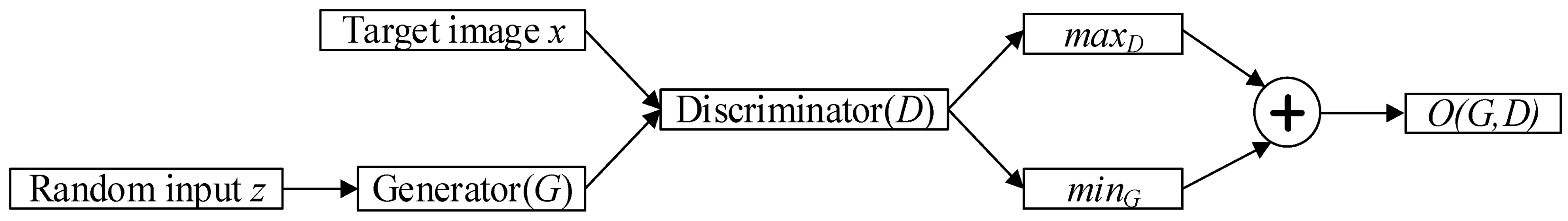
2.2. Generative Adversarial Network
2.3. Pix2Pix
2.4. CylcleGAN
2.5. Exposure Value GAN
3. Proposed Model
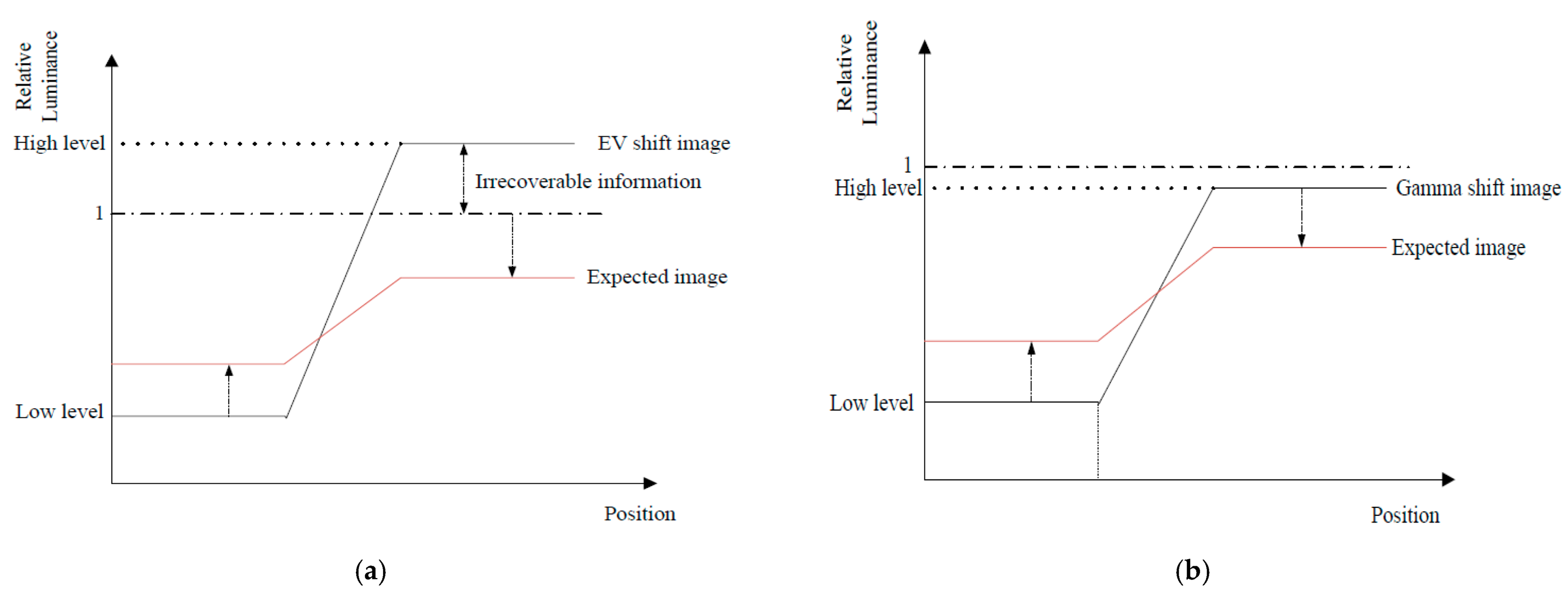
3.1. Motivation
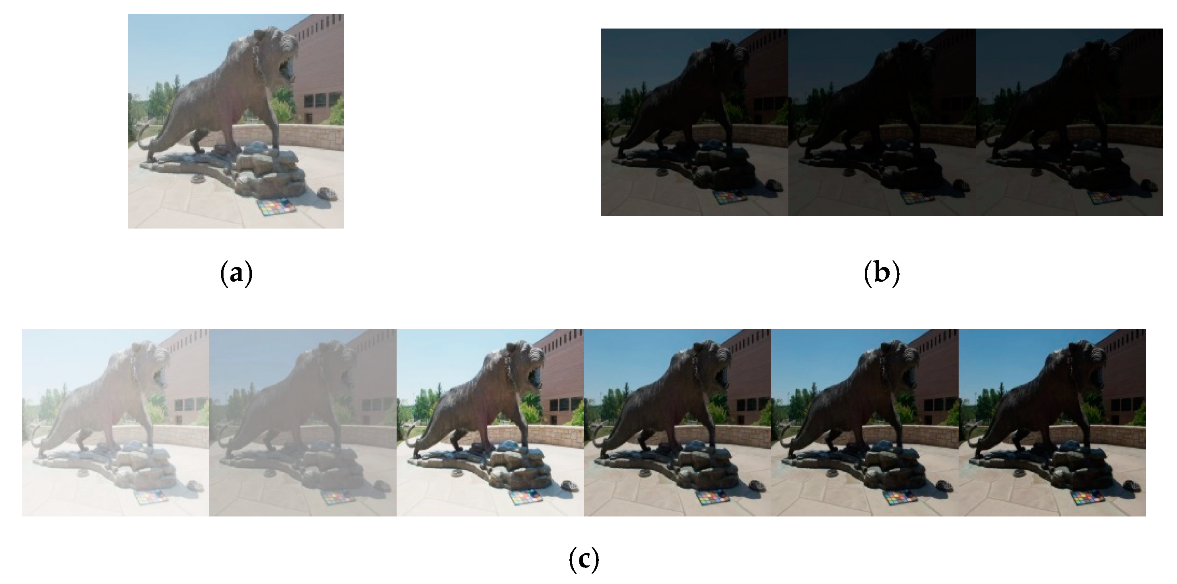
3.2. Gamma Shift Dataset for Tone Compression Generative Adversarial Network Training
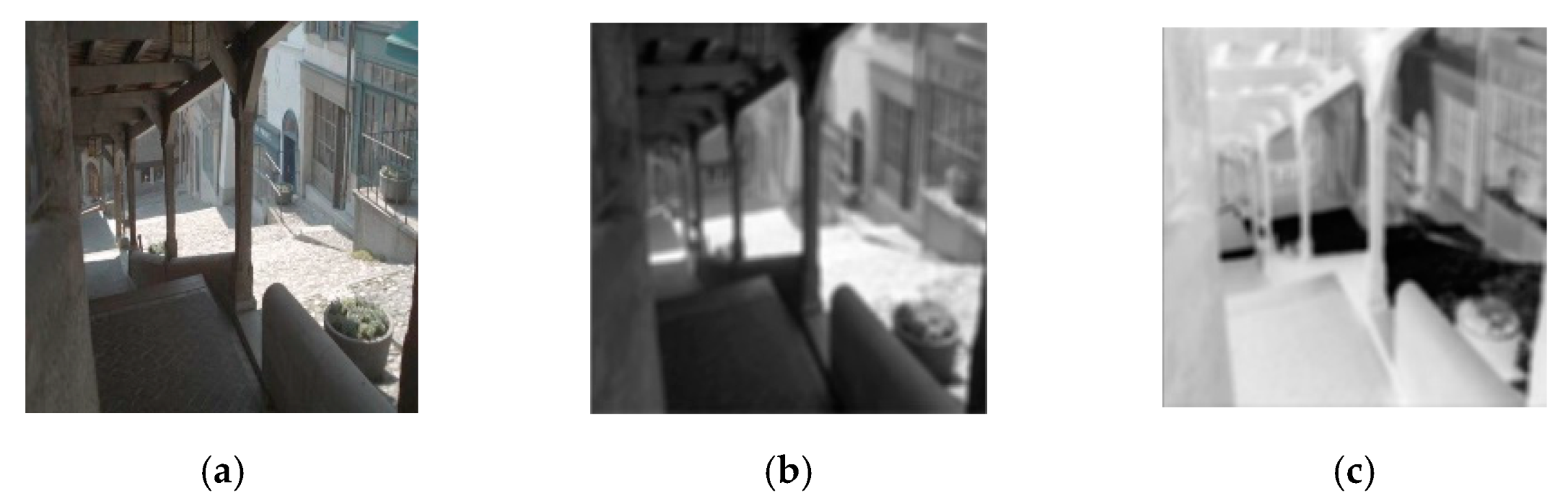
3.3. Regional Weighted Loss Function
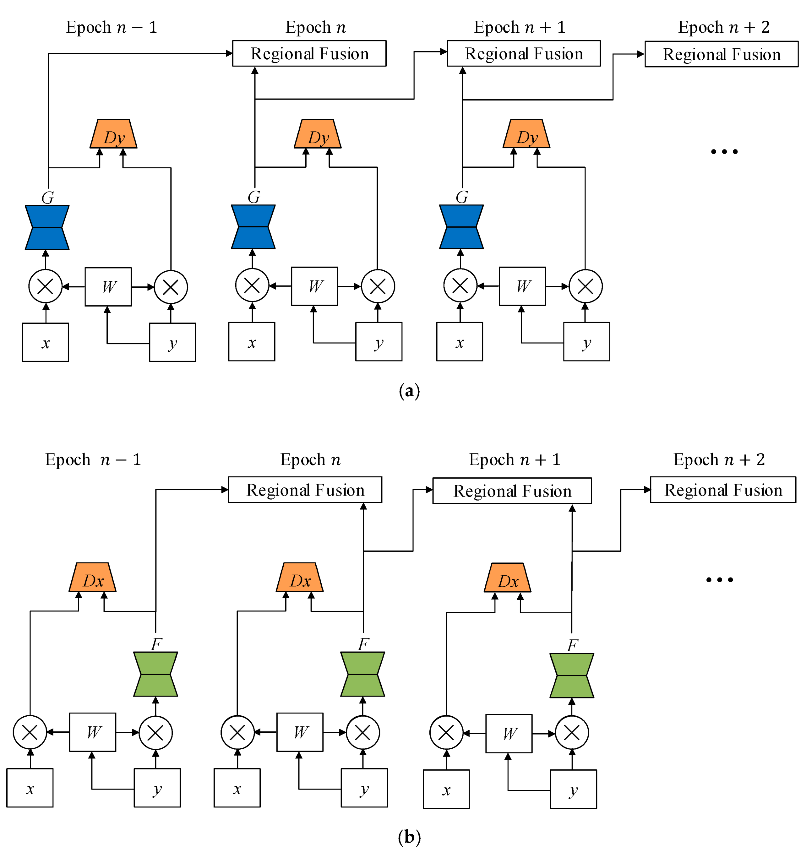
3.4. Regional Fusion Training
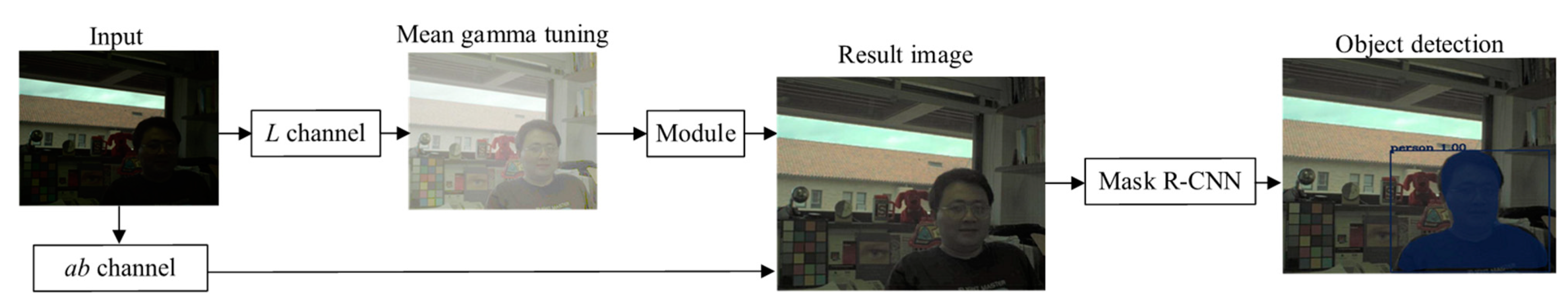
3.5. Mean Gamma Tunning
3.6. Architecture
4. Experiment Results
4.1. Enviroment
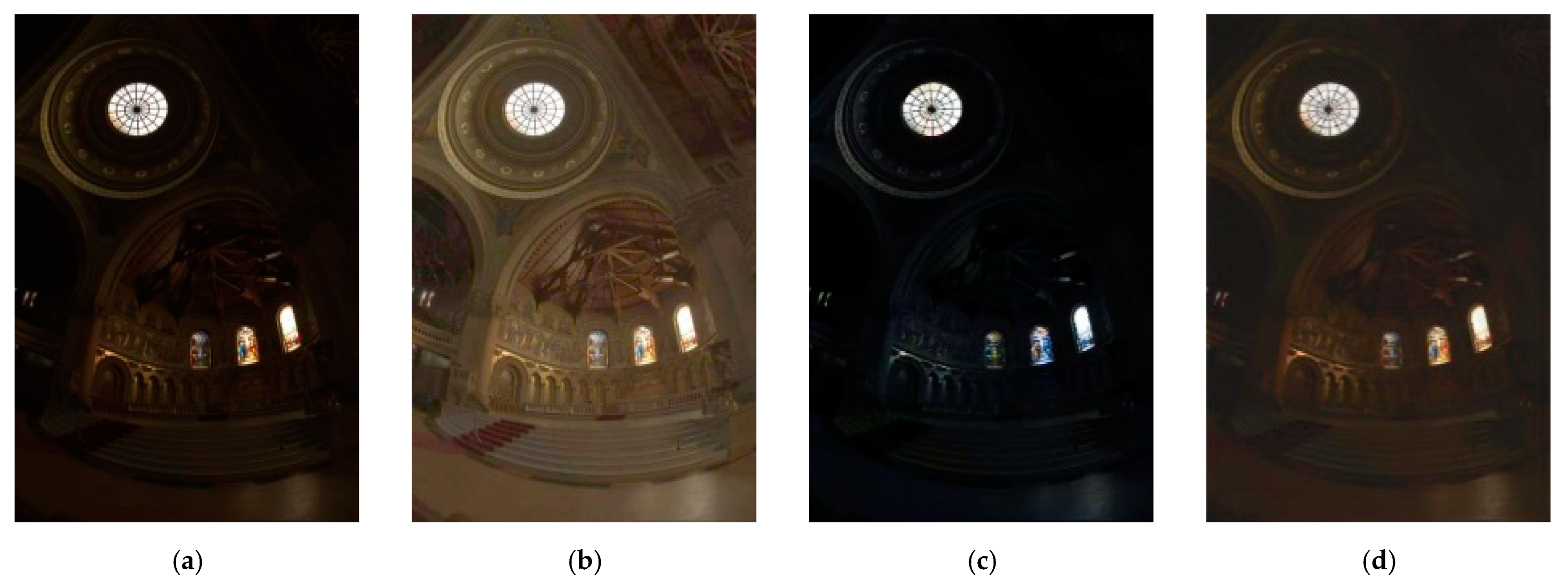
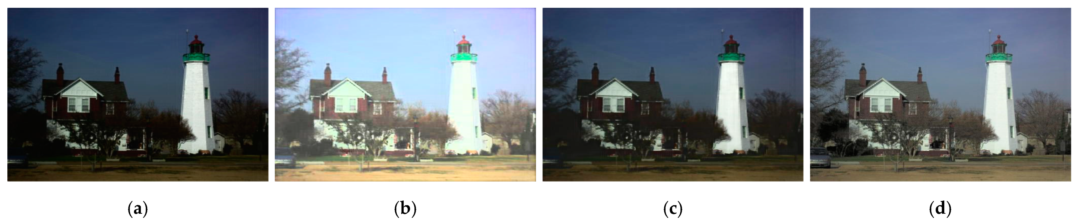
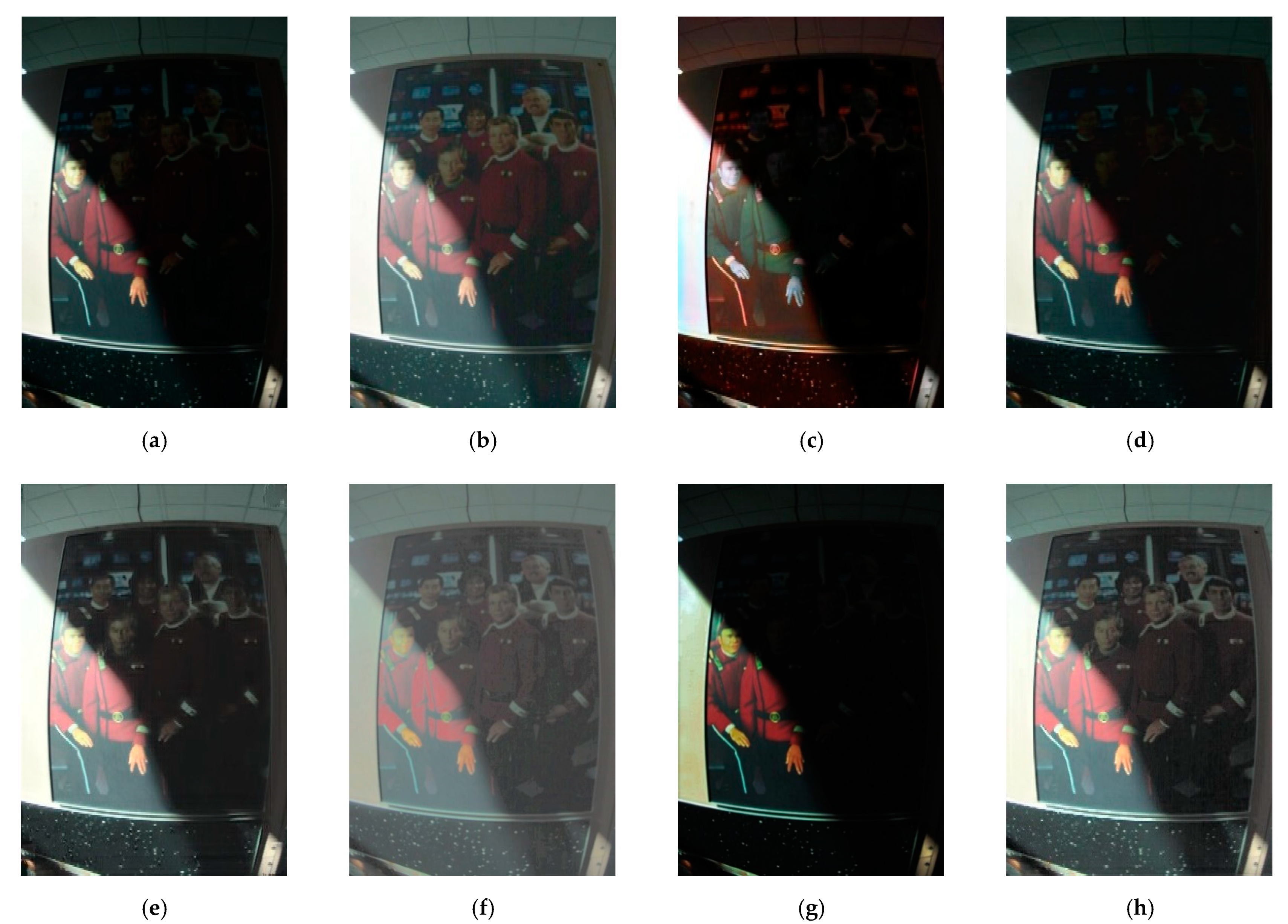
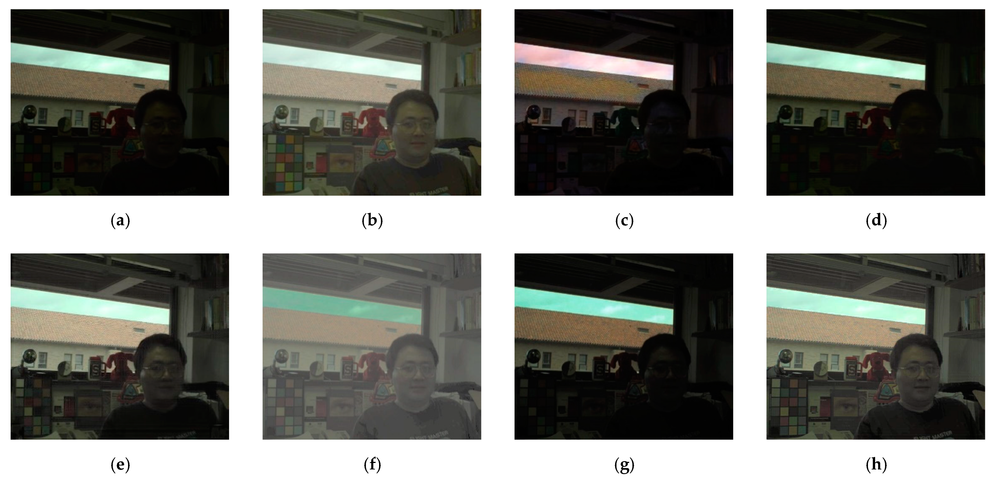
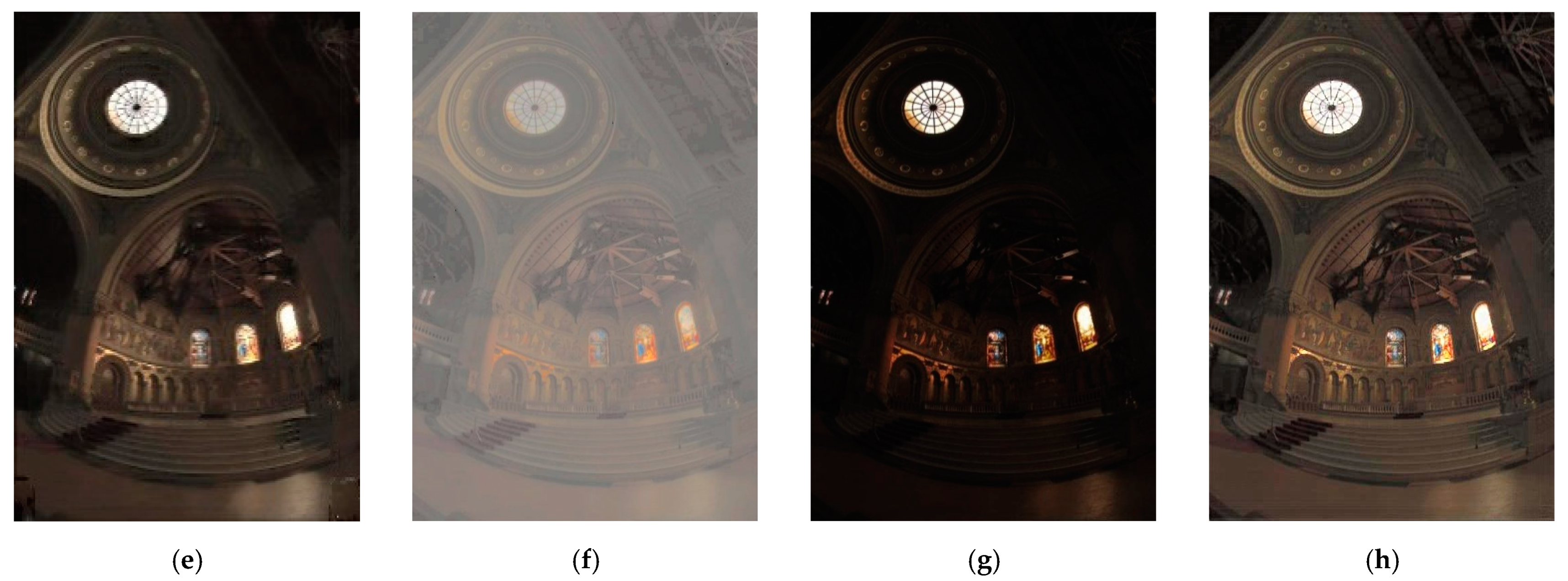
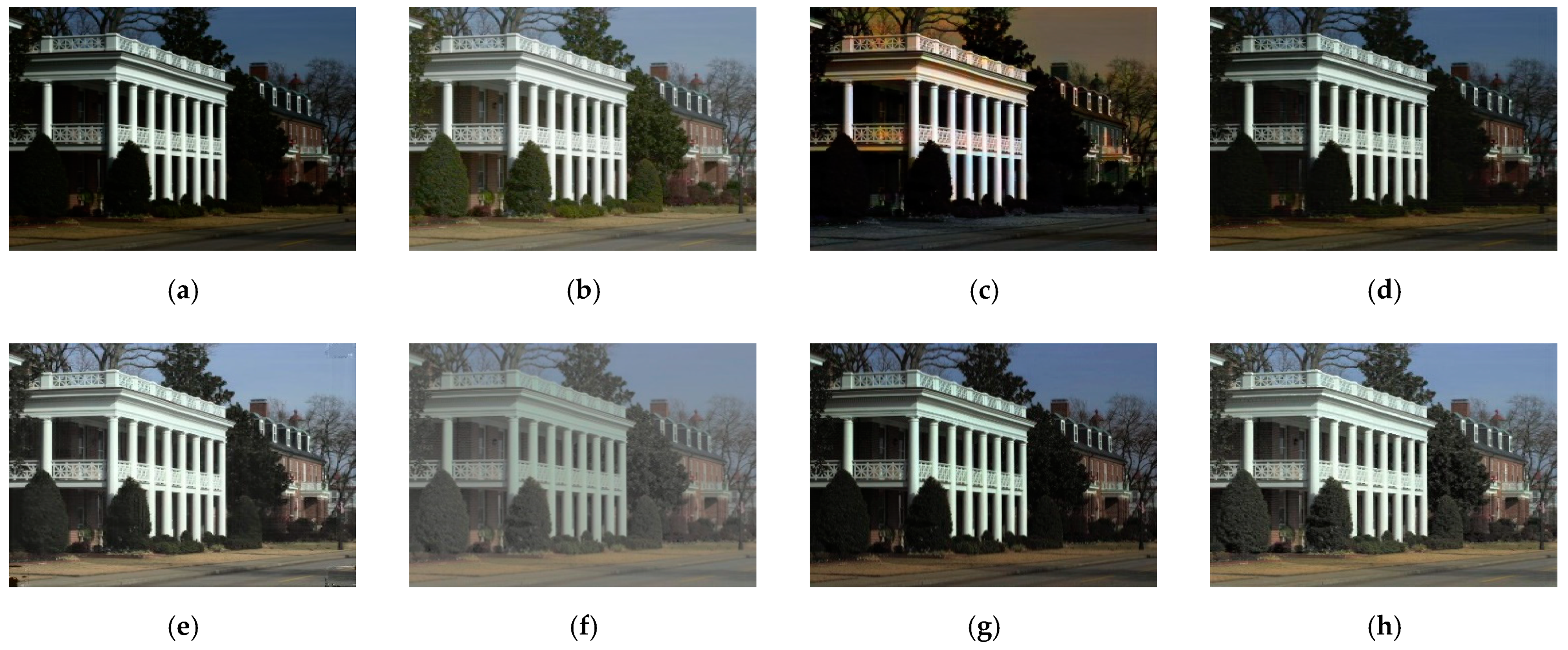
4.2. Step-by-Step Results of the Proposed Method
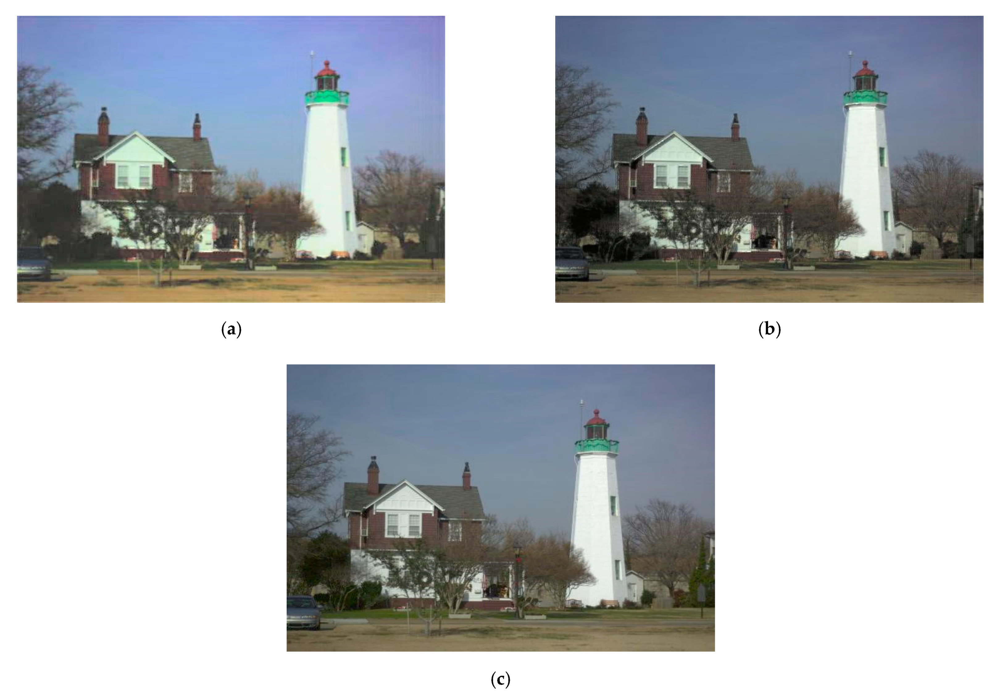
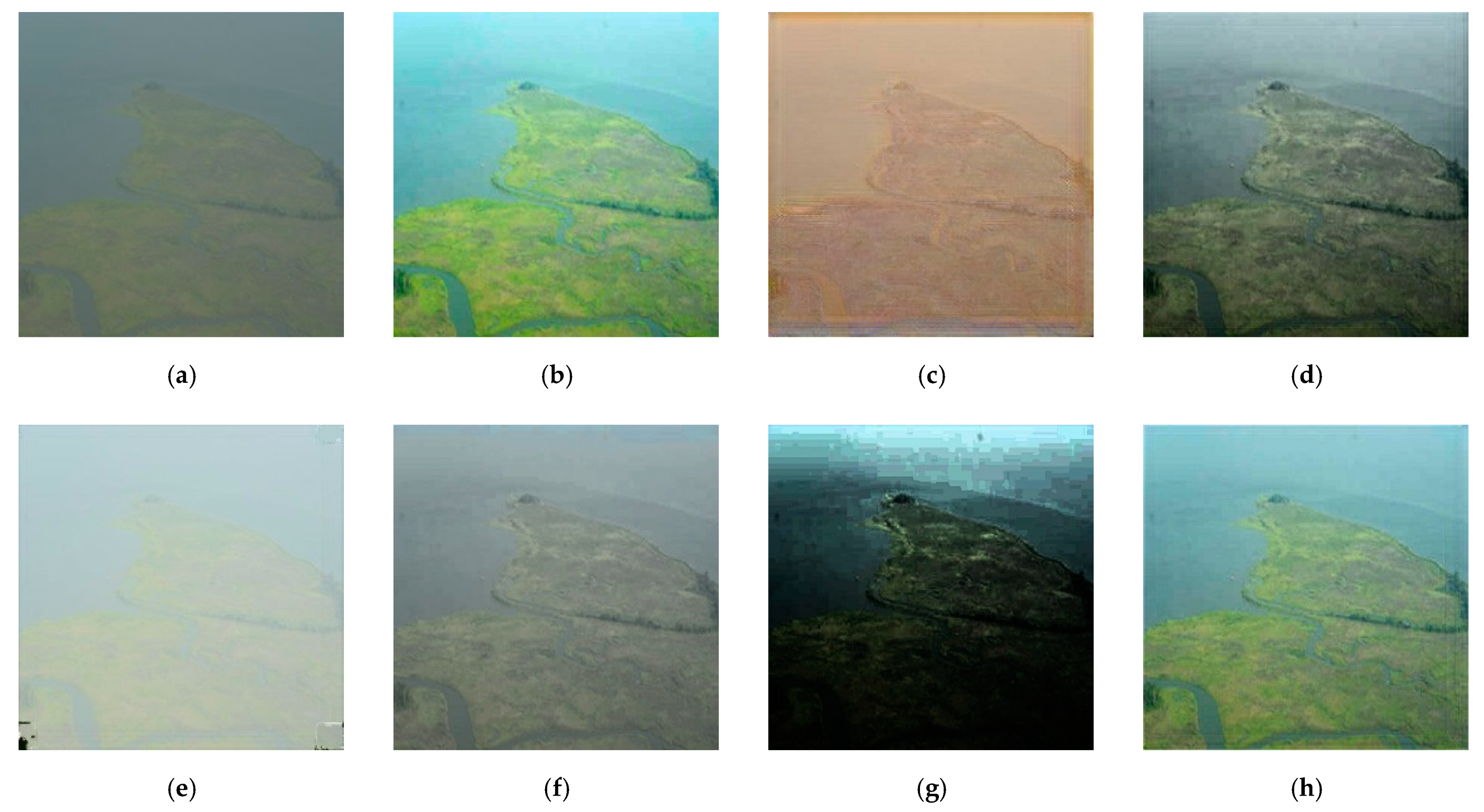
4.3. Comparison of Gamma Shift and Brigntness Augmentations
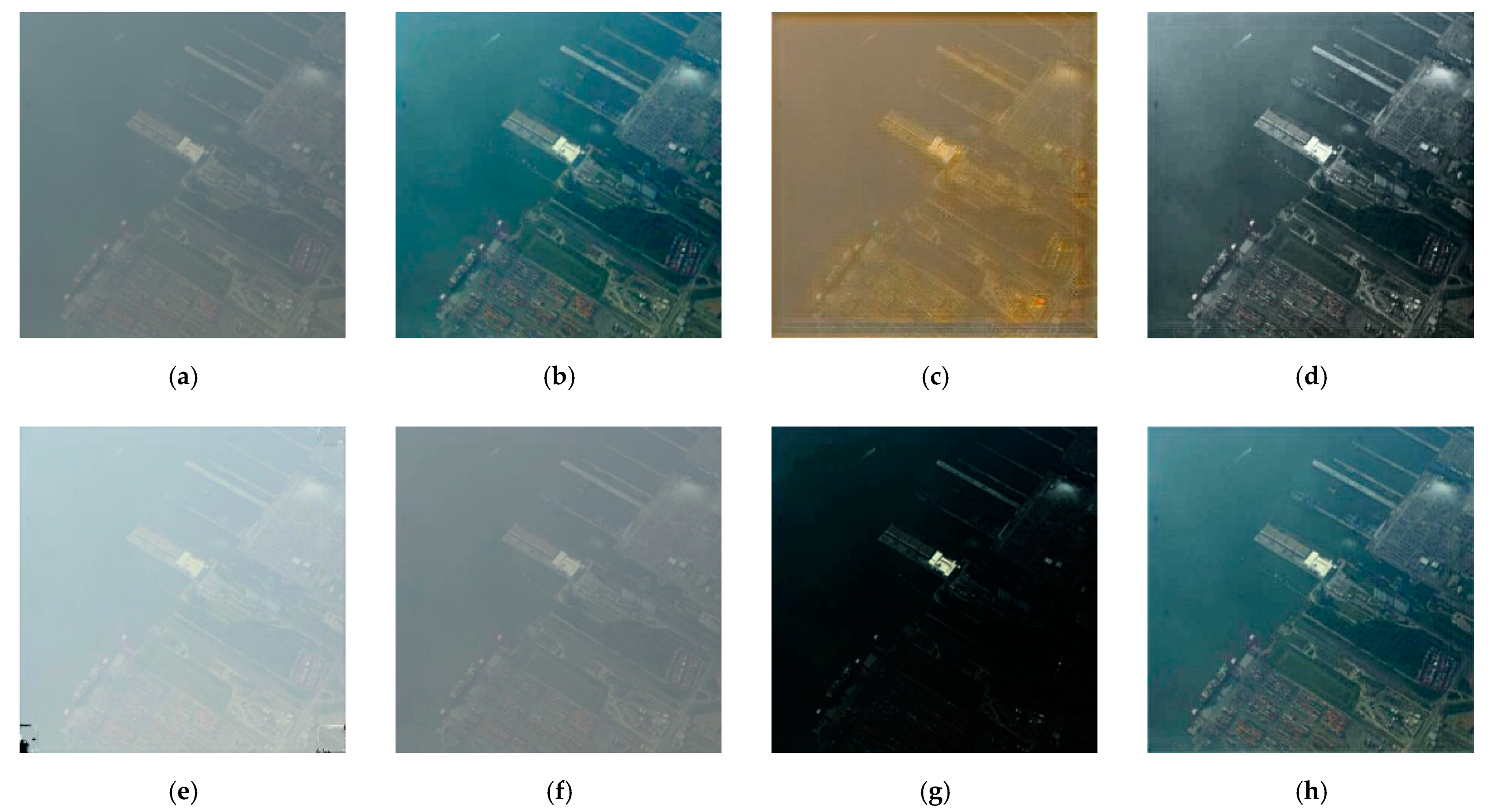
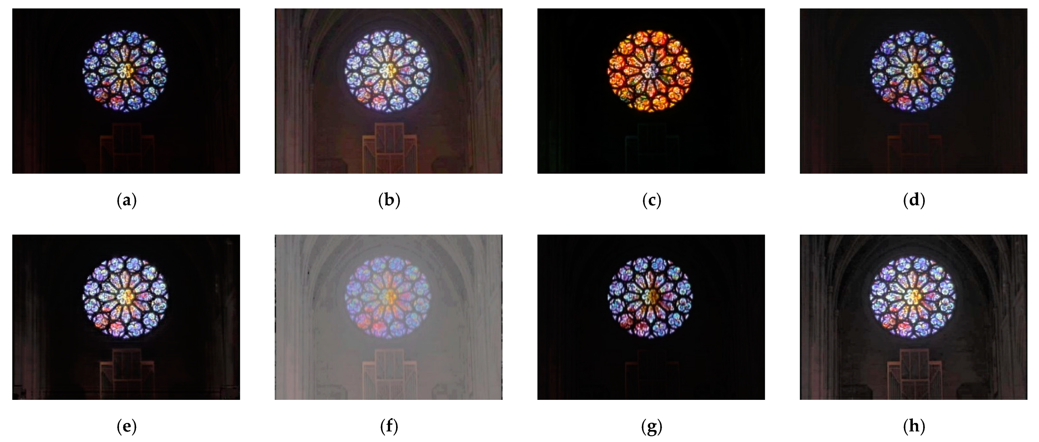
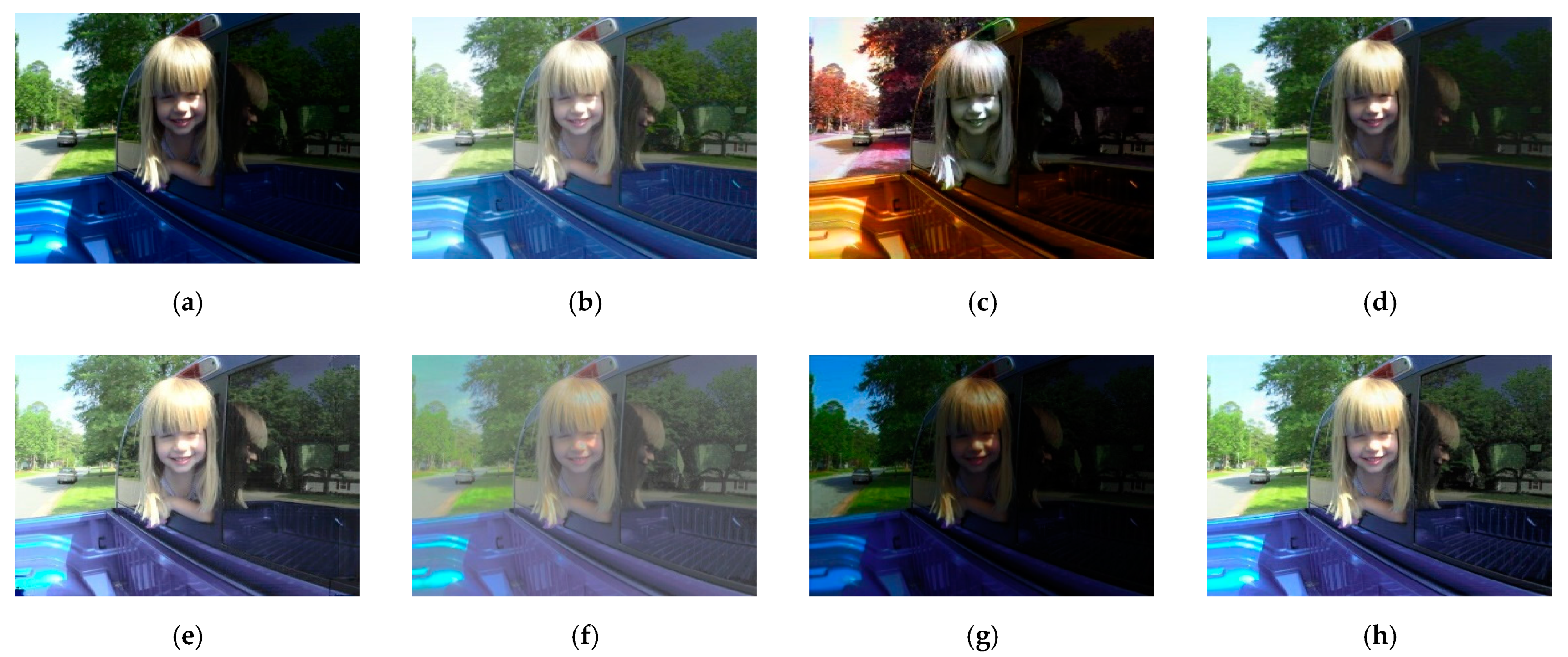
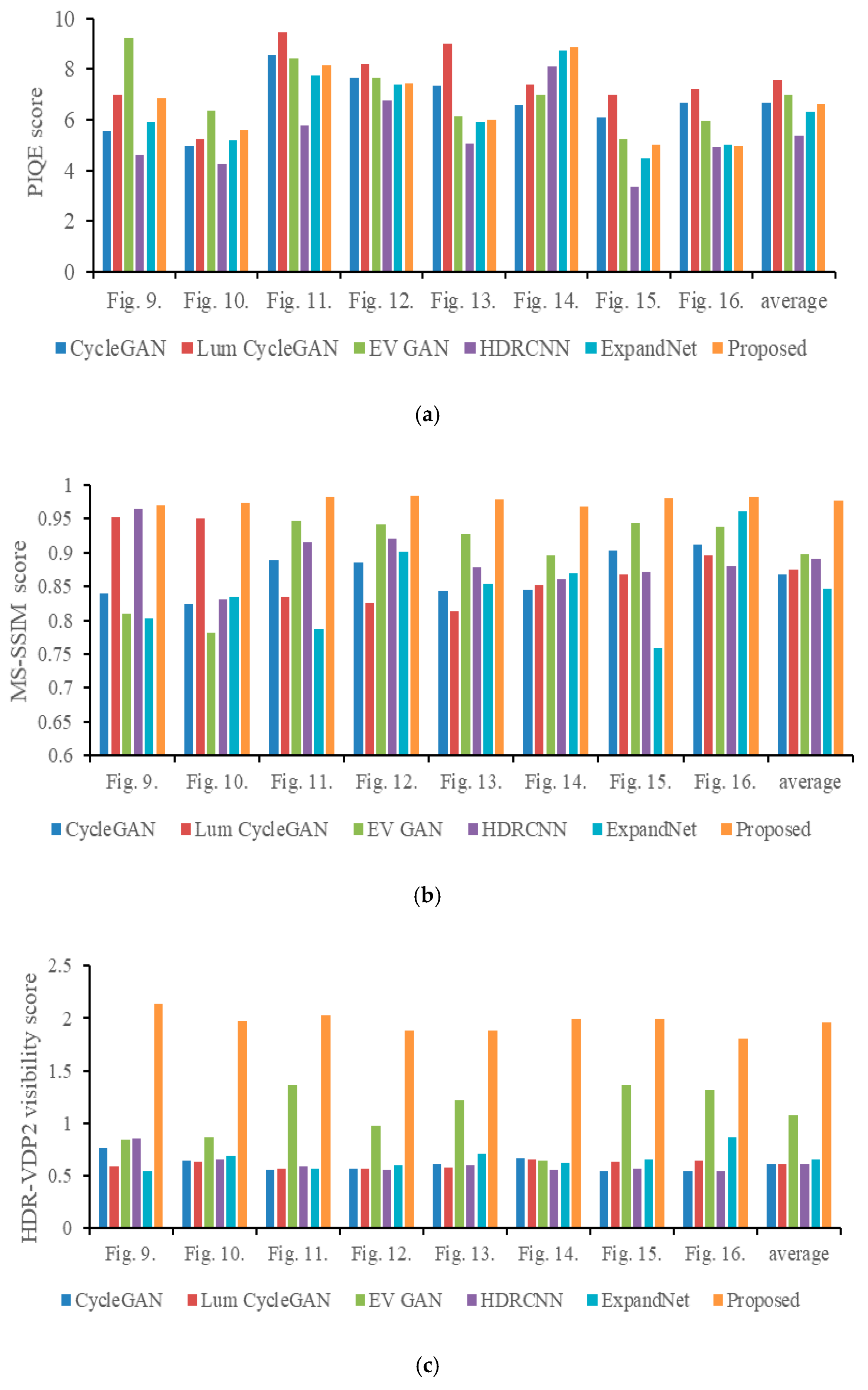
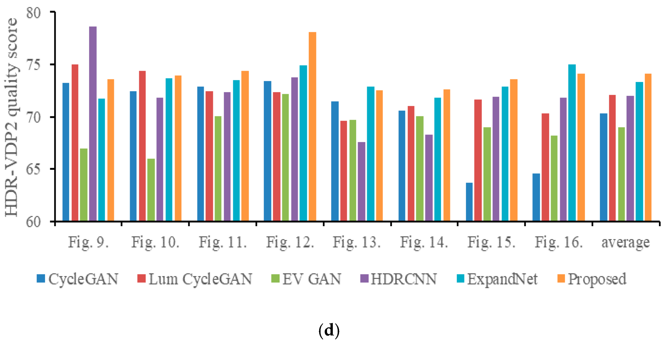
4.4. Comparisons with Conventional Methods
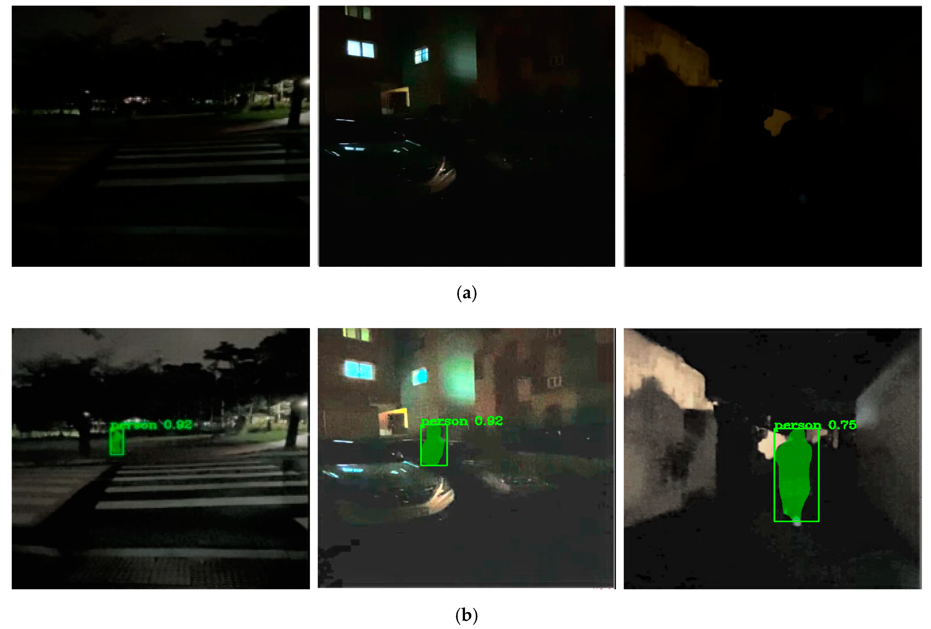
4.5. Object Detection Using Mask R-CNN
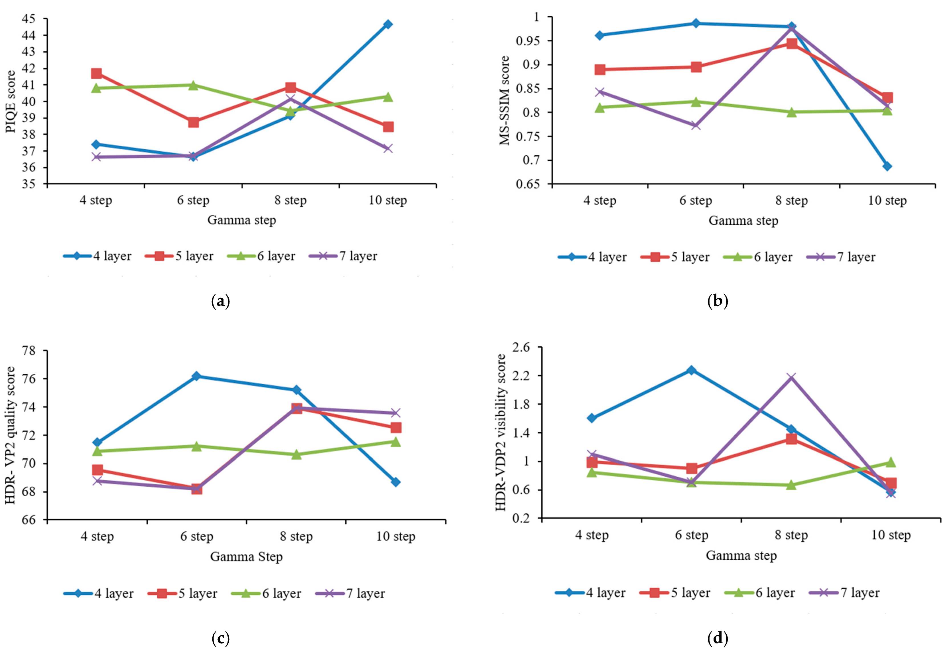
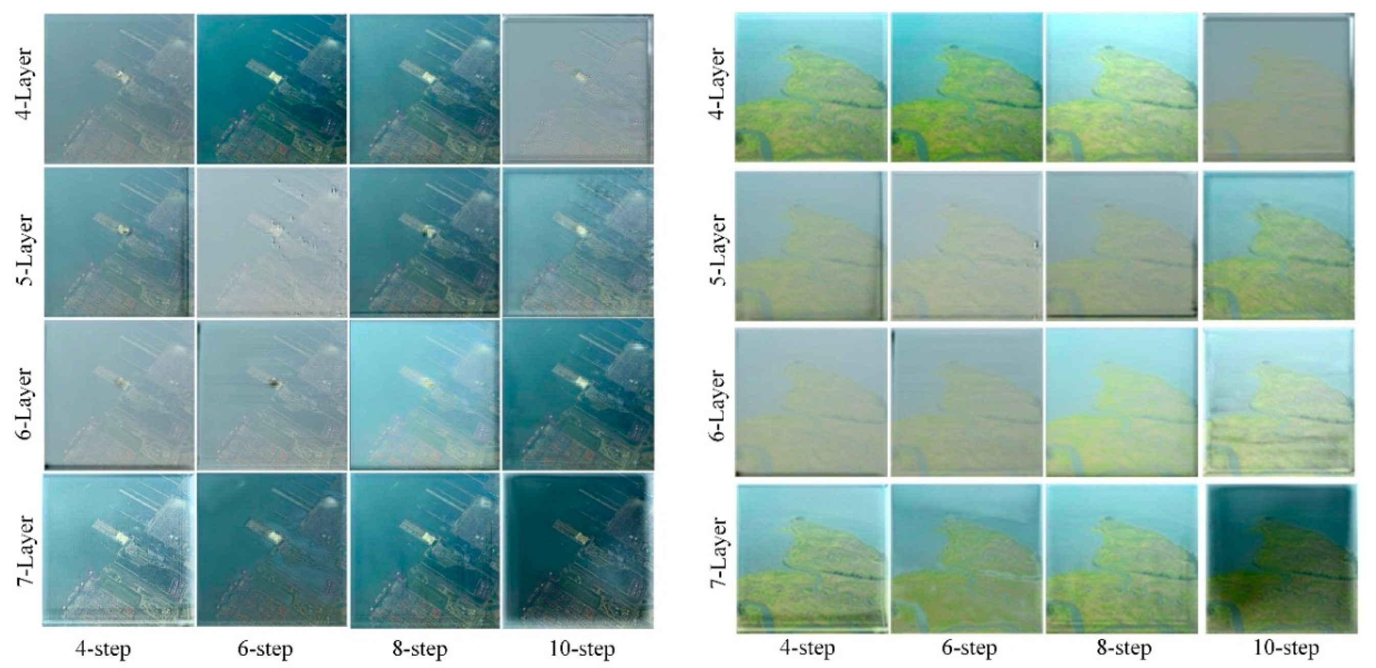
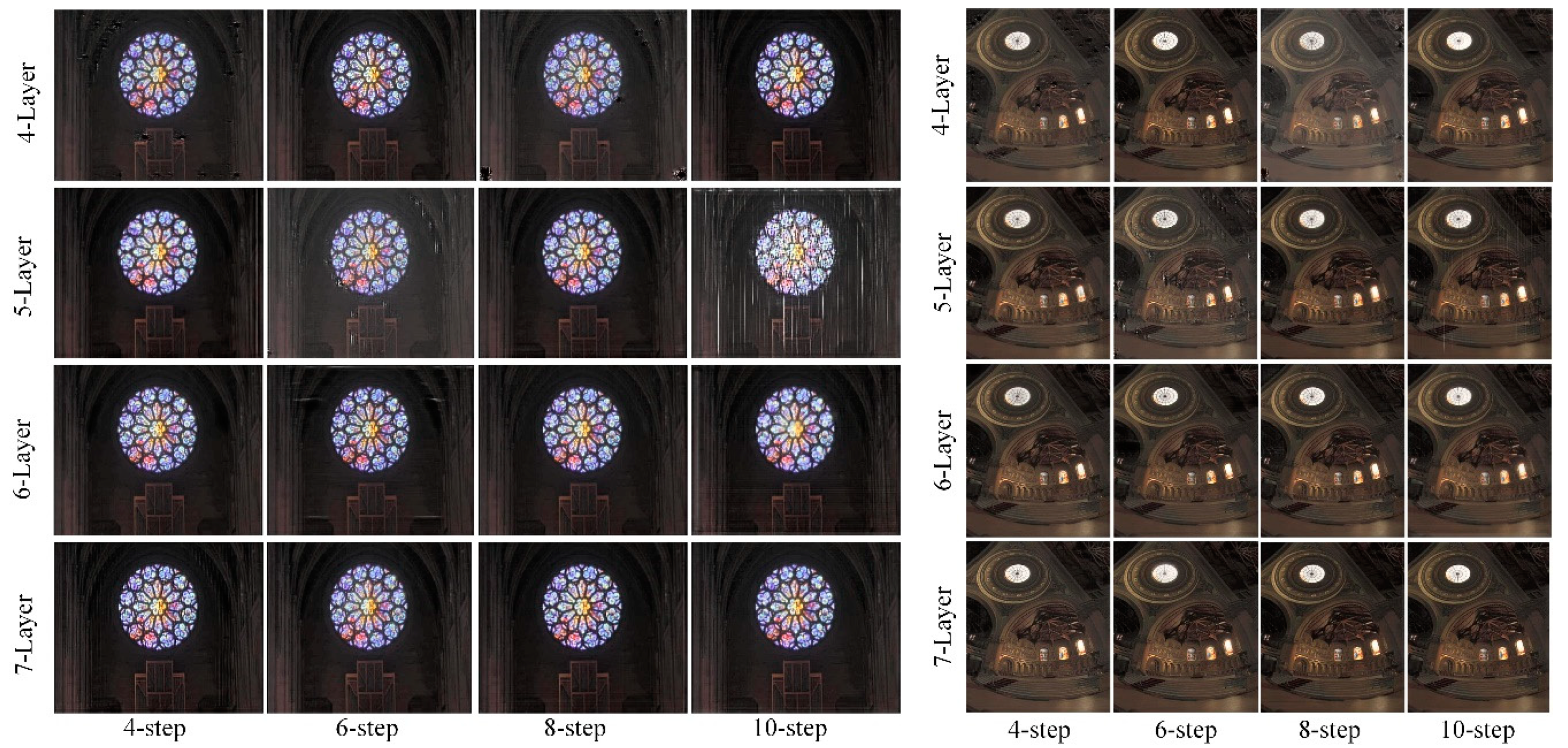
4.6. Parameter Optimization
5. Conclusions
Author Contributions
Funding
Institutional Review Board Statement
Informed Consent Statement
Data Availability Statement
Conflicts of Interest
References
- Debevec, P.E.; Malik, J. Recovering high dynamic range radiance maps from photographs. In Proceedings of the ACM SIGGRAPH 2008 Classes on-SIGGRAPH 2008, Los Angeles, CA, USA, 11–15 August 2008; p. 31. [Google Scholar] [CrossRef]
- Kwon, H.-J.; Lee, S.-H.; Lee, G.-Y.; Sohng, K.-I. Radiance map construction based on spatial and intensity correlations between LE and SE images for HDR imaging. J. Vis. Commun. Image Represent. 2016, 38, 695–703. [Google Scholar] [CrossRef]
- Banterle, F.; Ledda, P.; Debattista, K.; Chalmers, A. Inverse tone mapping. In Proceedings of the 4th International Conference on Computer Graphics and Interactive Techniques in Australasia and Southeast Asia, Kuala Lumpur, Malaysia, 29 November–2 December 2006; pp. 349–356. [Google Scholar] [CrossRef]
- Rempel, A.G.; Trentacoste, M.; Seetzen, H.; Young, H.D.; Heidrich, W.; Whitehead, L.; Ward, G. Ldr2Hdr: On-the-fly reverse tone mapping of legacy video and photographs. ACM Trans. Graph. 2007, 26, 39. [Google Scholar] [CrossRef]
- Huo, Y.; Yang, F.; Dong, L.; Brost, V. Physiological inverse tone mapping based on retina response. Vis. Comput. 2013, 30, 507–517. [Google Scholar] [CrossRef]
- Endo, Y.; Kanamori, Y.; Mitani, J. Deep reverse tone mapping. ACM Trans. Graph. 2017, 36, 1–10. [Google Scholar] [CrossRef]
- Eilertsen, G.; Kronander, J.; Denes, G.; Mantiuk, R.K.; Unger, J. HDR image reconstruction from a single exposure using deep CNNs. ACM Trans. Graph. 2017, 36, 178. [Google Scholar] [CrossRef]
- Marnerides, D.; Bashford-Rogers, T.; Hatchett, J.; Debattista, K. ExpandNet: A Deep Convolutional Neural Network for High Dynamic Range Expansion from Low Dynamic Range Content. Comput. Graph. Forum 2018, 37, 37–49. [Google Scholar] [CrossRef] [Green Version]
- Liu, Y.-L.; Lai, W.-S.; Chen, Y.-S.; Kao, Y.-L.; Yang, M.-H.; Chuang, Y.-Y.; Huang, J.-B. Single-Image HDR reconstruction by learning to reverse the camera pipeline. In Proceedings of the IEEE/CVF Conference on Computer Vision and Pattern Recognition (CVPR), Seattle, WA, USA, 13–19 June 2020; pp. 1648–1657. [Google Scholar] [CrossRef]
- Li, H.; Ma, K.; Yong, H.; Zhang, L. Fast Multi-Scale Structural Patch Decomposition for Multi-Exposure Image Fusion. IEEE Trans. Image Process. 2020, 29, 5805–5816. [Google Scholar] [CrossRef]
- Cai, J.; Gu, S.; Zhang, L. Learning a Deep Single Image Contrast Enhancer from Multi-Exposure Images. IEEE Trans. Image Process. 2018, 27, 2049–2062. [Google Scholar] [CrossRef] [PubMed]
- Wang, R.; Zhang, Q.; Fu, C.-W.; Shen, X.; Zheng, W.-S.; Jia, J. Underexposed photo enhancement using deep illumination estimation. In Proceedings of the IEEE/CVF Conference on Computer Vision and Pattern Recognition (CVPR), Long Beach, CA, USA, 16–20 June 2019; pp. 6842–6850. [Google Scholar] [CrossRef]
- LeCun, Y.; Boser, B.; Denker, J.S.; Henderson, D.; Howard, R.E.; Hubbard, W.; Jackel, L.D. Backpropagation Applied to Handwritten Zip Code Recognition. Neural Comput. 1989, 1, 541–551. [Google Scholar] [CrossRef]
- Isola, P.; Zhu, J.-Y.; Zhou, T.; Efros, A.A. Image-to-image translation with conditional adversarial networks. In Proceedings of the IEEE Conference on Computer Vision and Pattern Recognition (CVPR), Honolulu, HI, USA, 21–26 July 2017; pp. 5967–5976. [Google Scholar] [CrossRef] [Green Version]
- Zhu, J.-Y.; Park, T.; Isola, P.; Efros, A.A. Unpaired image-to-image translation using cycle-consistent adversarial networks. In Proceedings of the IEEE International Conference on Computer Vision (ICCV), Venice, Italy, 22–29 October 2017; pp. 2242–2251. [Google Scholar] [CrossRef] [Green Version]
- Kuang, J.; Johnson, G.M.; Fairchild, M.D. iCAM06: A refined image appearance model for HDR image rendering. J. Vis. Commun. Image Represent. 2007, 18, 406–414. [Google Scholar] [CrossRef]
- Jung, S.-W.; Son, D.-M.; Kwon, H.-J.; Lee, S.-H. Regional weighted generative adversarial network for LDR to HDR image conversion. In Proceedings of the International Conference on Artificial Intelligence in Information and Communication (ICAIIC), Fukuoka, Japan, 19–21 February 2020; pp. 697–700. [Google Scholar] [CrossRef]
- Jung, S.-W.; Kwon, H.-J.; Son, D.-M.; Lee, S.-H. Generative Adversarial Network Using Weighted Loss Map and Regional Fusion Training for LDR-to-HDR Image Conversion. IEICE Trans. Inf. Syst. 2020, 103, 2398–2402. [Google Scholar] [CrossRef]
- He, K.; Gkioxari, G.; Dollár, P.; Girshick, R. Mask R-CNN. IEEE Trans. Pattern Anal. Mach. Intell. 2020, 42, 386–397. [Google Scholar] [CrossRef] [PubMed]
- Krizhevsky, A.; Sutskever, I.; Hinton, G.E. ImageNet classification with deep convolutional neural networks. Commun. ACM 2017, 60, 84–90. [Google Scholar] [CrossRef]
- Wollmer, M.; Blaschke, C.; Schindl, T.; Schuller, B.; Farber, B.; Mayer, S.; Trefflich, B. Online Driver Distraction Detection Using Long Short-Term Memory. IEEE Trans. Intell. Transp. Syst. 2011, 12, 574–582. [Google Scholar] [CrossRef] [Green Version]
- Chen, Y.-S.; Wang, Y.-C.; Kao, M.-H.; Chuang, Y.-Y. Deep photo enhancer: Unpaired learning for image enhancement from photographs with GANs. In Proceedings of the IEEE/CVF Conference on Computer Vision and Pattern Recognition, Salt Lake City, UT, USA, 18–22 June 2018; pp. 6306–6314. [Google Scholar] [CrossRef]
- Iizuka, S.; Simo-Serra, E.; Ishikawa, H. Let there be color! Joint end-to-end learning of global and local image priors for automatic image colorization with simultaneous classification. ACM Trans. Graph. 2016, 35, 110. [Google Scholar] [CrossRef]
- Bengio, Y. Learning Deep Architectures for AI. Found. Trends Mach. Learn. 2009, 2, 1–127. [Google Scholar] [CrossRef]
- Zhang, Y.; Tian, Y.; Kong, Y.; Zhong, B.; Fu, Y. Residual dense network for image super-resolution. In Proceedings of the IEEE Conference on Computer Vision and Pattern Recognition, Salt Lake City, UT, USA, 18–22 June 2018. [Google Scholar] [CrossRef] [Green Version]
- Wu, S.; Zhong, S.-H.; Liu, Y. Deep residual learning for image steganalysis. Multimed. Tools Appl. 2017, 77, 10437–10453. [Google Scholar] [CrossRef]
- Retinex Images. Available online: https://dragon.larc.nasa.gov (accessed on 11 November 2019).
- Fairchild, M.D. HDR Dataset. Available online: http://rit-mcsl.org/fairchild//HDR.html (accessed on 6 June 2019).
- Moorthy, A.K.; Bovik, A. Blind Image Quality Assessment: From Natural Scene Statistics to Perceptual Quality. IEEE Trans. Image Process. 2011, 20, 3350–3364. [Google Scholar] [CrossRef] [PubMed]
- Wang, Z.; Simoncelli, E.P.; Bovik, A.C. Multi-scale structural similarity for image quality assessment. In Proceedings of the Thrity-Seventh Asilomar Conference on Signals, Systems & Computers, Pacific Grove, CA, USA, 9–12 November 2003. [Google Scholar] [CrossRef] [Green Version]
- Mantiuk, R.; Kim, K.J.; Rempel, A.G.; Heidrich, W. HDR-VDP-2: A calibrated visual metric for visibility and quality predictions in all luminance conditions. ACM Trans. Graph. 2011, 30, 40. [Google Scholar] [CrossRef]
- Chen, Z.; Zeng, Z.; Shen, H.; Zheng, X.; Dai, P.; Ouyang, P. DN-GAN: Denoising generative adversarial networks for speckle noise reduction in optical coherence tomography images. Biomed. Signal Process. Control 2019, 55, 101632. [Google Scholar] [CrossRef]


| Method | Time(s) |
|---|---|
| CycleGAN | 0.398 |
| Lum CycleGAN | 0.334 |
| EV GAN | 0.339 |
| HDRCNN | 1.006 |
| ExpandNet | 0.267 |
| Proposed model | 0.339 |
Publisher’s Note: MDPI stays neutral with regard to jurisdictional claims in published maps and institutional affiliations. |
© 2021 by the authors. Licensee MDPI, Basel, Switzerland. This article is an open access article distributed under the terms and conditions of the Creative Commons Attribution (CC BY) license (https://creativecommons.org/licenses/by/4.0/).
Share and Cite
Jung, S.-W.; Kwon, H.-J.; Lee, S.-H. Enhanced Tone Mapping Using Regional Fused GAN Training with a Gamma-Shift Dataset. Appl. Sci. 2021, 11, 7754. https://doi.org/10.3390/app11167754
Jung S-W, Kwon H-J, Lee S-H. Enhanced Tone Mapping Using Regional Fused GAN Training with a Gamma-Shift Dataset. Applied Sciences. 2021; 11(16):7754. https://doi.org/10.3390/app11167754
Chicago/Turabian StyleJung, Sung-Woon, Hyuk-Ju Kwon, and Sung-Hak Lee. 2021. "Enhanced Tone Mapping Using Regional Fused GAN Training with a Gamma-Shift Dataset" Applied Sciences 11, no. 16: 7754. https://doi.org/10.3390/app11167754
APA StyleJung, S.-W., Kwon, H.-J., & Lee, S.-H. (2021). Enhanced Tone Mapping Using Regional Fused GAN Training with a Gamma-Shift Dataset. Applied Sciences, 11(16), 7754. https://doi.org/10.3390/app11167754