Soft Sensor Transferability: A Survey

Abstract

Soft Sensors (SSs) are inferential dynamical models employed in industries to perform prediction of process hard-to-measure variables based on their relation with easily accessible ones. They allow implementation of real-time control and monitoring of the plants and present other advantages in terms of costs and efforts. Given the complexity of industrial processes, these models are generally designed with data-driven black-box machine learning (ML) techniques. ML methods work well only if the data on which the prediction is performed share the same distribution with the one on which the model was trained. This is not always possible, since plants can often show new working conditions. Even similar plants show different data distributions, making SSs not scalable between them. Models should then be created from scratch with highly time-consuming procedures. Transfer Learning (TL) is a field of ML that re-uses the knowledge from one task to learn a new different, but related, one. TL techniques are mainly used for classification tasks. Only recently TL techniques have been adopted in the SS field. The proposed survey reports the state of the art of TL techniques for nonlinear dynamical SSs design. Methods and applications are discussed and the new directions of this research field are depicted.

1. Introduction

The advent of Industry 4.0 improved the automation and monitoring of traditional manufacturing and process industries [1]. Implementing efficient plant monitoring and control policies is performed through measurement acquisition and data elaboration systems.

Models of real industrial processes, able to perform prediction of process variables by exploiting their dependence on other ones, are known as Soft Sensors (SSs) [2,3].

Machine Learning (ML) and Deep Learning (DL) have greatly increased the capabilities of such data-driven systems over the last few years in the industrial automation field [4]. However, the practical implementation of those techniques is hampered by two characteristics of ML [5,6]. The first is that the training dataset and the actual system variables have to share the same feature space and the same distribution to perform prediction properly: collected data must be capable of representing the whole dynamics of the system since the model cannot provide more information than the that stored in the training data themselves. This means that training data have to be very large and varied to be able to represent uncommon occurrences too.

In an industrial environment, data acquisition already poses a limitation, since production systems and industrial processes cannot be stopped to perform experiments and generate suitable learning data. Ad-hoc experiments are indeed difficult, time-consuming and costly. For this reason, the SS designer refers to data stored in the historical databases which always contains outliers, multi-rate acquisitions, and suffer from labeled data scarcity [4].

The second ML characteristic refers to model retraining which is needed to cope with time-varying process and signal drift [7]. This could be sometimes comparable to training a new model from scratch, requiring large amounts of computational power and large datasets. Moreover, either in presence of new working conditions or when new processes are considered, the number of available data is too low to design a new model [8].

Nowadays, the gaps between domains and distributions of data and changes in the processes are the main obstacles of ML techniques for SS modelling for complex industrial processes.

The reported issues can be mitigated by Transfer Learning (TL), a set of approaches, increasingly popular in the ML field, which take advantage of the knowledge already acquired by a model on a source task to transfer it to a target task [9]. TL would allow reduction in the amount and quality of data needed by transferring knowledge among tasks. TL can also be used to approach model scalability from a process to a similar one [10,11].

TL has increasingly gained attention since the issue of inconsistency of data distribution is a common barrier in many general ML applications. TL was then been applied to different fields, as reviewed by different publications, such as in medical imaging [12], email spam [13] and speech recognition [14]. On the other side, in the industrial automation field, it still is a new research topic. Most of the studies focus on classification problems, anomaly detection, fault diagnosis and quality monitoring [15]. Only in the last two years have applications of TL methods for SSs design appeared in the literature.

This survey covers the recent developments of TL techniques to nonlinear dynamical SSs design. Methods and applications reported in the recent literature are discussed along with the description of the future trends in the field.

The remaining of the paper is organized as follows: firstly, a brief description of SSs and their design procedure is given in Section 2 to explain the need of TL; the main TL methodologies are then introduced in Section 3; in Section 4 current applications of TL methods for SSs are examined and classified. Final discussions and future trends are drawn in Section 5.

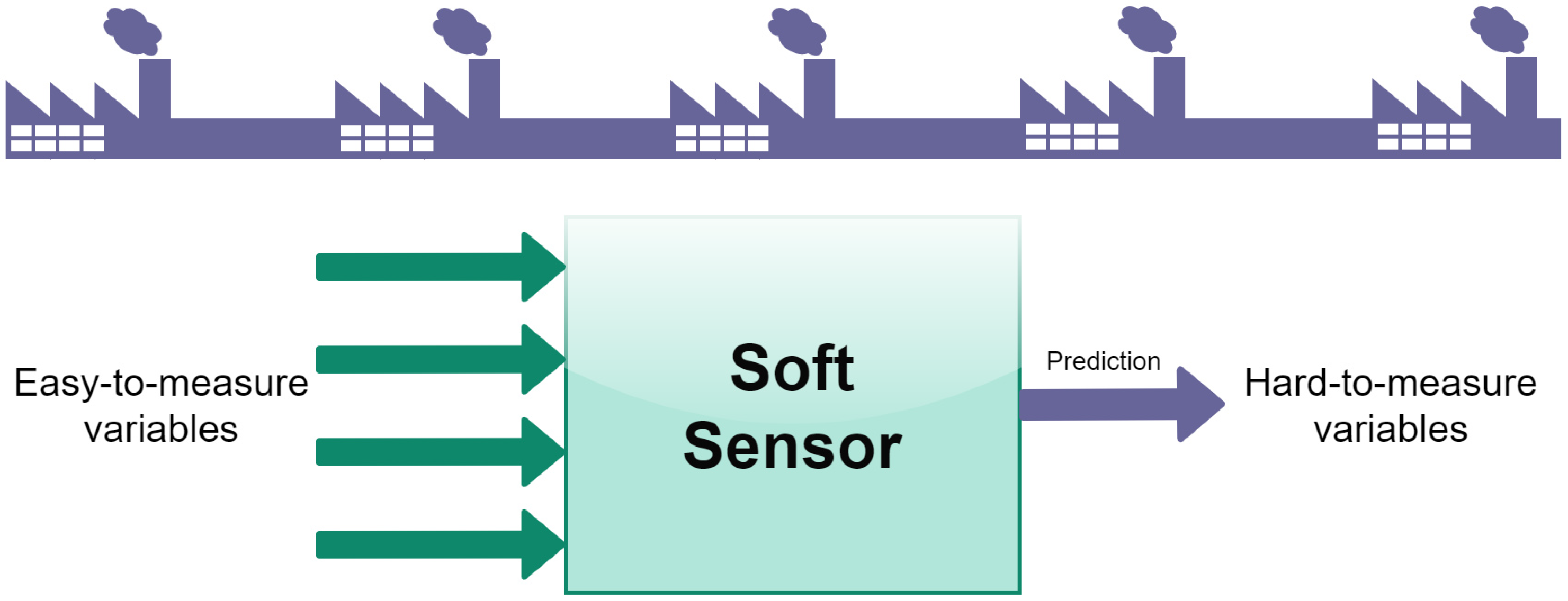
2. Soft Sensors

In industrial plants, many variables are monitored through online sensors. There are cases though in which some of them cannot be measured online due to the lack of online measurement instruments or hostile environments. This requires frequent sensor maintenance and/or introduces high delays due to laboratory analysis. SSs can be a solution to these issues. They are inferential models that make use of the underlying relations between the accessible process variables to provide an estimation of the required hard-to-measure physical variables as schematized in Figure 1.

Depending on the problem complexity an, SS can be realized by using static/dynamic, linear/nonlinear, time-invariant/variant models [2]. SSs allow for real-time plant control, measuring system back-up, what-if analysis, sensor validation and fault diagnosis as well [3,16].

SSs, also named as virtual sensors, are adopted in different fields such as refineries [17,18], chemical plants [19], cement kilns [20], power plants [21], pulp and paper mills [22], food processing [23], polymerization processes [24], and wastewater treatment systems [25].

SSs can be designed by using first principle models when a priori physical knowledge of the plant is given [3]. When such knowledge is not available, or the modelling process is overcomplicated, the design of SSs relies on data-driven black-box techniques [26].

Data-driven SS design is a highly time-consuming task that involves pattern recognition [27] and system identification [28] steps, as summarized in the following:

• Data collection and filtering;
• Input variables selection;
• Model choice;
• Model identification;
• Model validation.

Data are retrieved from industries’ historical databases and must be selected to represent the whole dynamics of the system. Historical databases usually suffer from oversampling, outliers, missing data, offsets, seasonal effects and high-frequency noise. An accurate pre-processing is therefore needed for the successive step of input selection, in which highly informative inputs concerning the chosen output are selected among the many available inputs [29].

The model choice should be conducted taking into consideration different characteristics, i.e., linear/nonlinear, static/dynamic, time-variant/invariant. Linear models, in general, do not show good performances for industrial processes. Nonlinear models are therefore widely used.

The following model classes for linear systems are usually considered:

$$y\left(t\right)=G\left(z^{-1}\right)u\left(t\right)+H\left(z^{-1}\right)e\left(t\right),$$

(1)

where $G(·)$ and $H(·)$ are transfer functions, $z^{-1}$ is the time delay operator and $e\left(t\right)$ a white noise signal. The identification procedure aims at determining a good estimate of $G(·)$ and $H(·)$, so the model can produce one-step-ahead predictions with a low variance error. The one-step-ahead predictor can be written in its regressor form as:

$$\widehat{y}\left(t\right|t-1,\theta )=\phi \left(t\right)\theta ,$$

(2)

where $\theta$ is the parameter vector and $\phi$ the regression vector that can contain past samples of system inputs and outputs and/or residuals. The model is then determined by identifying the parameters of the transfer functions. Models; structures are defined by imposing the structure of the transfer functions i.e., of the regression vector. The main parametric structure families are

• FIR, characterized by the following regression vector:

  $$\phi \left(t\right)={[u(t-d)\dots u(t-d-m)]}^T,$$

  (3)

  with d and m being the delay of the samples;
• ARX, characterized by the following regression vector:

  $$\phi \left(t\right)={[y(t-1),\dots ,y(t-l),u(t-d),\dots ,u(t-d),u(t-d-m)]}^T;$$

  (4)

  where l is the maximum delay needed for the output variables;
• ARMAX, characterized by the following regression vector:

  $$\begin{array}{cc}\hfill \phi (t,\theta )=& \left[y\right(t-1),\dots ,y(t-l),u(t-d),\dots ,u(t-d-m),u(t-d-m),\hfill \\ & {,\epsilon (t,\theta ),\dots ,\epsilon (t-k,\theta )]}^T.\hfill \end{array}$$

  where $\epsilon$ is the model residual and k is the associated maximum time delay.

The linear structures above can be extended to their nonlinear counterparts, respectively NFIR, NARX, NARMAX where a nonlinear function is considered between the regressor vector and the estimated output. For data-driven designed SSs, these model structures can be implemented with a wide variety of ML techniques such as Artificial Neural Networks (ANN) [30], Convolutional Neural Networks (CNN) [31], Generative Adversarial Networks (GAN) [32], Deep Belief Networks (DBN) [33], Support Vector Regression (SVR) [34], Gaussian Processes Regression (GPR) [35], just to mention a few.

Finally, the identification step allows empirical estimation of the model unknown parameters based on the training dataset, whereas the validation step exploits test data to verify whether the model can adequately represent the system and be generalized to new samples.

Data-driven ML methods give better performance under the common assumption that training data and test data share the same distribution [5]. This characteristic should also be maintained during the future use of the SS.

The problem of data distribution inconsistency between the training and the test phases can be mitigated by the adoption of TL techniques. TL is a research field in ML that aims to exploit the knowledge gained while learning a task (source domain) to learn a different but related one (target domain) more efficiently [9].

This means that such techniques can handle the problem of data distribution inconsistency between the training and the test phases. Nevertheless, even though such techniques gained success more than ten years ago, little attention has been paid to their application to the SS field and process systems monitoring.

Few studies have employed TL methods in the fault detection and diagnosis of industrial systems, as reported in Maschler and Weyrich [15], and in regression problems for condition monitoring purposes [36]. Only in the last year have new results appeared in the literature addressing the application of TL techniques to SSs.

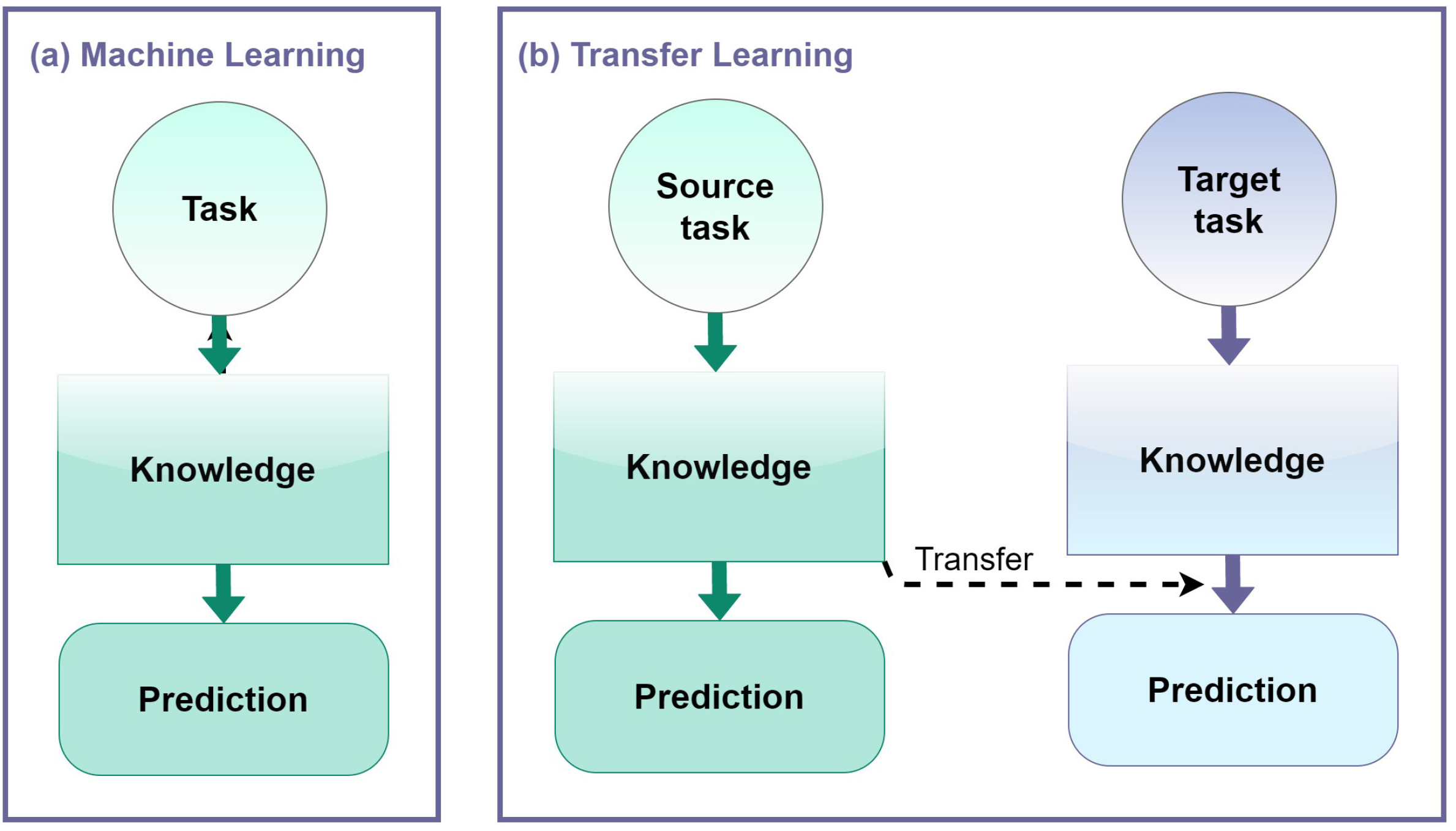
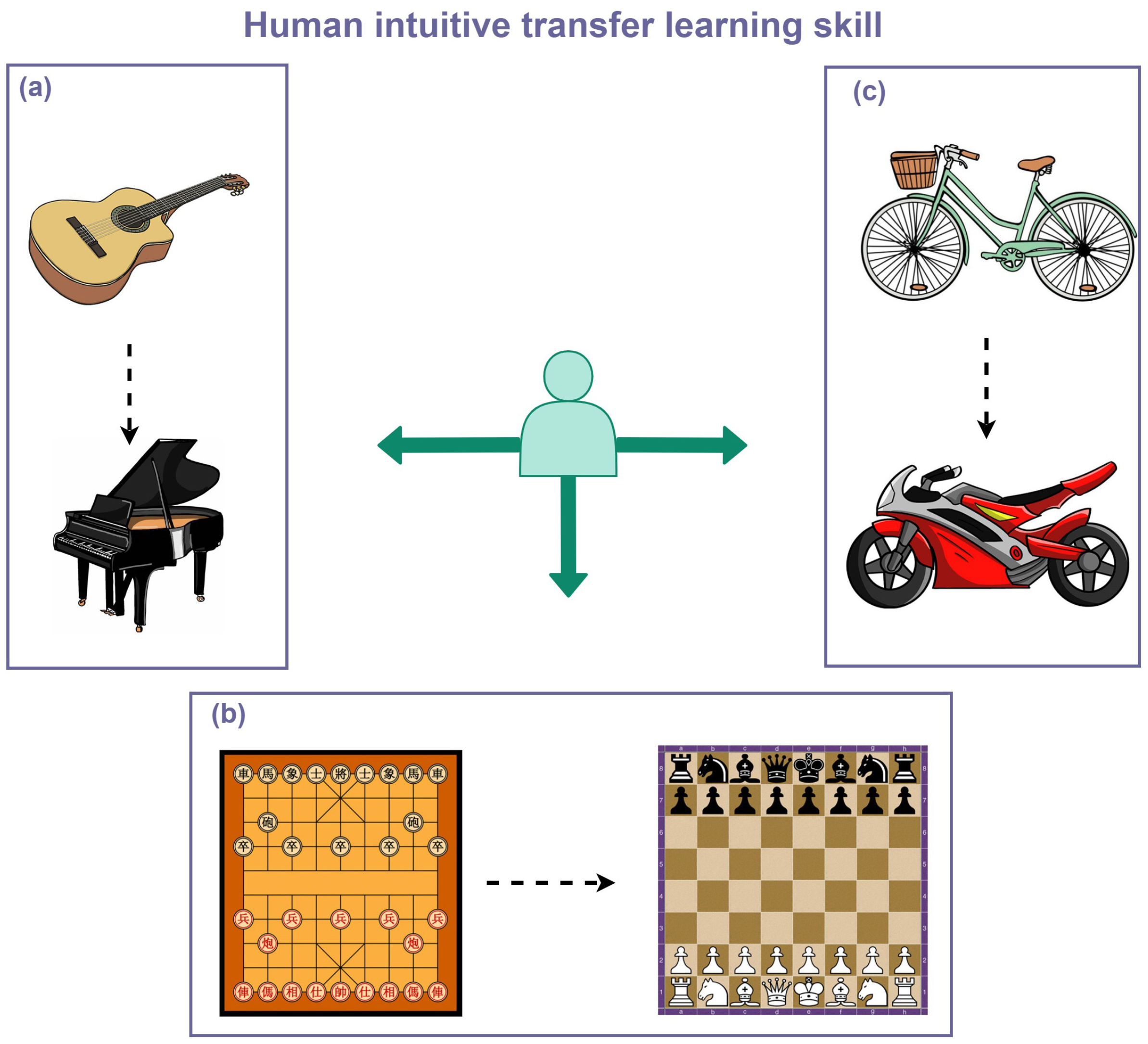
3. Transfer Learning

As stated before, TL methodologies are useful when the data distribution of the target domain is different from the data distribution of the source domain [9].

Figure 2 shows the difference in the learning process in cases of traditional ML and TL.

In the first case, the task is learned from scratch each time, while in the TL case the knowledge acquired from a previously learned source task is, in some way, transferred while learning a target task, to overcome scarcity in high-quality target data.

A practical and common example is given by the problem of sentiment classification, which consists of a classification task on reviews of a specific type of product as a positive or negative view. To train the classifier, many reviews are first collected and labeled. When the type of product changes, such a classifier will not maintain good performance, if the distribution of data differs from the previous product. This means that new data should be collected and labeled for each type of product to create a new classifier. Such a procedure indeed being very expensive, TL techniques allow use of a classification model trained for some specific products to adapt to others of a different type, saving a great amount of effort [37].

Many other examples of TL are observable in nature as well, as shown in Figure 3.

Humans themselves can intelligently apply the knowledge previously learned from one task to solve new ones faster or more efficiently. For instance, the knowledge acquired by learning a musical instrument would allow one to learn a new instrument faster.

Formal definitions to introduce the TL problem will now be provided.

Given a feature space $\mathcal{X}$, an instance set X defined as $X=\left\{x_1,\dots ,x_n\right\}\in \mathcal{X}$ and its marginal probability distribution $P\left(X\right)$, a domain$\mathcal{D}$ is defined as

$$\mathcal{D}=\left\{\mathcal{X},P\left(X\right)\right\}.$$

(5)

This means that two domains differ when either their $\mathcal{X}$ or $P\left(X\right)$ differ.

Given a domain $\mathcal{D}$, a prediction, or a task, $\mathcal{T}$ is defined by a label space $\mathcal{Y}$ and a predictive function $f(·)$ as

$$\mathcal{T}=\left\{\mathcal{Y},f(·)\right\}.$$

(6)

This again implies that two tasks differ when either their $\mathcal{Y}$ or $f(·)$ differ. The predictive function $f(·)$ is not known a priori, but learned from the training data, which consist of the labeled pairs $\left\{x_i,y_i\right\}$, where $x_i\in X,y_i\in \mathcal{Y}$, with $i=1\dots ,n$. Given a new instance x, then $f(·)$ can be used to predict its corresponding label $f\left(x\right)$, that from a probabilistic point of view can be written as $P\left(y\right|x)$.

In the TL problem, distinction is made between a source domain ${\mathcal{D}}_{\mathcal{S}}$ and its corresponding source task${\mathcal{T}}_{\mathcal{S}}$; a target domain${\mathcal{D}}_{\mathcal{T}}$ and its target task${\mathcal{T}}_{\mathcal{T}}$.

The source domain ${\mathcal{D}}_{\mathcal{S}}$ is usually observed via the instance–label pairs as

$$D_{\mathcal{S}}=\left\{\left(x_{{\mathcal{S}}_1},y_{{\mathcal{S}}_1}\right)\dots ,\left(x_{{\mathcal{S}}_{n_{\mathcal{S}}}},y_{{\mathcal{S}}_{n_{\mathcal{S}}}}\right)\right\},where{x}_{{\mathcal{S}}_i}\in {\mathcal{X}}_{\mathcal{S}}and{y}_{{\mathcal{S}}_i}\in {\mathcal{Y}}_{\mathcal{S}}.$$

(7)

Whereas, the target domain data are denoted as

$$D_{\mathcal{T}}=\left\{\left(x_{{\mathcal{T}}_1},y_{{\mathcal{T}}_1}\right),\dots ,\left(x_{{\mathcal{T}}_{n_{\mathcal{T}}}},y_{{\mathcal{T}}_{n_{\mathcal{T}}}}\right)\right\},where{x}_{{\mathcal{T}}_i}\in {\mathcal{X}}_{\mathcal{T}}and{y}_{{\mathcal{T}}_i}\in {\mathcal{Y}}_{\mathcal{T}}.$$

(8)

In most real applications, an observation of the target domain consists of unlabeled instances or just a limited number of labeled ones, meaning that usually $0\le n_{\mathcal{T}}\ll n_{\mathcal{S}}$.

TL aims to improve the learning of the target predictive function $f_{\mathcal{T}}(·)$ in ${\mathcal{D}}_{\mathcal{T}}$ using the knowledge in ${\mathcal{D}}_{\mathcal{S}}$ and ${\mathcal{T}}_{\mathcal{S}}$, where ${\mathcal{D}}_{\mathcal{S}}\ne {\mathcal{D}}_{\mathcal{T}}$, ${\mathcal{T}}_{\mathcal{S}}\ne {\mathcal{T}}_{\mathcal{T}}$.

When the target and source domains are the same, ${\mathcal{D}}_{\mathcal{S}}={\mathcal{D}}_{\mathcal{T}}$, and their tasks are the same, ${\mathcal{T}}_{\mathcal{S}}={\mathcal{T}}_{\mathcal{T}}$, then it becomes an usual ML problem.

As already stated, the condition ${\mathcal{D}}_{\mathcal{S}}\ne {\mathcal{D}}_{\mathcal{T}}$ implies that

$${\mathcal{X}}_{\mathcal{S}}\ne {\mathcal{X}}_{\mathcal{T}}orP\left(X_{\mathcal{S}}\right)\ne P\left(X_{\mathcal{T}}\right).$$

(9)

Analogously, $\mathcal{T}$ being defined as $\mathcal{T}=\left\{\mathcal{Y},P\left(Y\right|X)\right\}$, the condition ${\mathcal{T}}_{\mathcal{S}}\ne {\mathcal{T}}_{\mathcal{T}}$ means that

$${\mathcal{Y}}_{\mathcal{S}}\ne {\mathcal{Y}}_{\mathcal{T}}orP\left(Y_{\mathcal{S}}\right|X_{\mathcal{S}})\ne P\left(Y_{\mathcal{T}}\right|X_{\mathcal{T}}).$$

(10)

Finally, when there exists some kind of relationship between the feature spaces of the two domains, then the domains are said to be related. In some cases, when the two domains are not related, a knowledge transfer could be unsuccessful at the point of worsening the learning in the target domain. When the target learner is indeed hurt by the transfer, the phenomenon is referred to as negative transfer [38].

The above definitions allow performance a categorization of TL techniques. Approaches can be grouped on a different basis, in particular under a problem point of view and an approach point of view. In the first case, the categorization can be performed on either the presence of labels in the source and target datasets (label setting) or the consistency of the feature space (space setting); the latter categorizes the types of TL techniques based on “what” part of the knowledge from the source is actually transferred to the target. The classification is reported in

Table 1. Most commonly adopted categorizations of TL techniques, under a “problem” point of view and an “approach” point of view.

TL Categories
Categorization Criterion		Types
Problem categorization	Label setting	Inductive Transductive Unsupervised
	Space setting	Homogeneous Heterogeneous
Approach categorization	“What” is transferred	Instance-based Feature-based Parameter-based Relational-based

and described in detail as follows.

From the label-setting aspect, TL techniques can be categorized into three types, based on the possible different situations between domains and tasks of the source and the target: inductive transfer learning, transductive transfer learning, unsupervised transfer learning (see Figure 4).

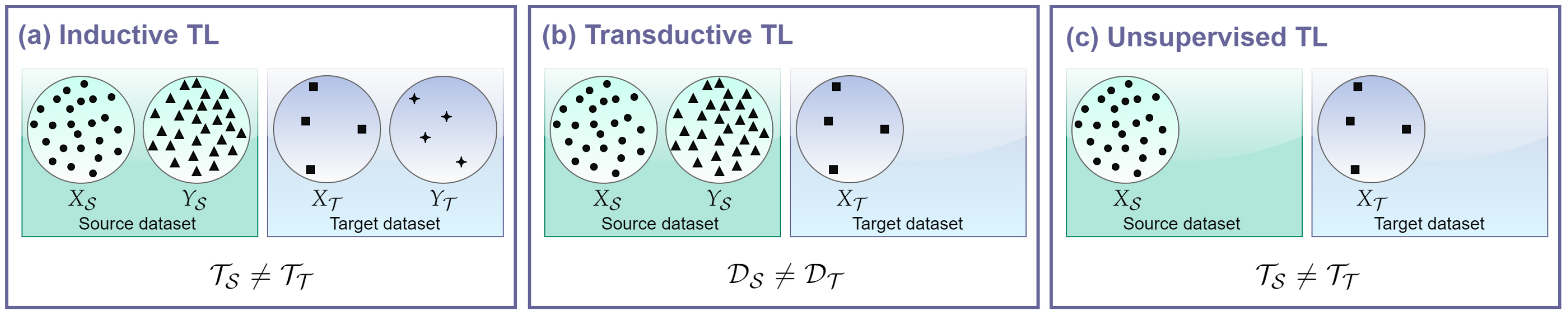
• Inductive TL: target and source tasks are different, regardless of the domains, and the label information of the target domain instances is available. Target-labeled data induce the learning of the target predictive model, hence the name;
• Transductive TL: target and source domains differ and the label information only comes from the source domain. In this case, if the domains differ because the feature spaces are the same ${\mathcal{X}}_{\mathcal{S}}={\mathcal{X}}_{\mathcal{T}}$, but the marginal probability distributions of the inputs differ $P\left(X_{\mathcal{S}}\right)\ne P\left(X_{\mathcal{T}}\right)$, such TL setting is referred to as domain adaptation [39];
• Unsupervised TL: target and source tasks are different and the label information is unknown for both the source and the target domains. This means that by definition such setting regards clustering and dimensionality reduction tasks, and not classification or regression as in the previous cases. For this reason, given the application of SSs, unsupervised solutions are not considered.

Another categorization is based on the consistency between the feature and label spaces from the source and the target.

• Homogeneous TL: if ${\mathcal{X}}_{\mathcal{S}}={\mathcal{X}}_{\mathcal{T}}$ and/or ${\mathcal{Y}}_{\mathcal{S}}={\mathcal{Y}}_{\mathcal{T}}$;
• Heterogeneous TL: if ${\mathcal{X}}_{\mathcal{S}}\ne {\mathcal{X}}_{\mathcal{T}}$ and/or ${\mathcal{Y}}_{\mathcal{S}}\ne {\mathcal{Y}}_{\mathcal{T}}$.

Besides the label settings or the consistency of the spaces, TL techniques can be categorized based on “what” is transferred, leading to four groups: instance-based, feature-based, parameter-based and relational-based (see Figure 5).

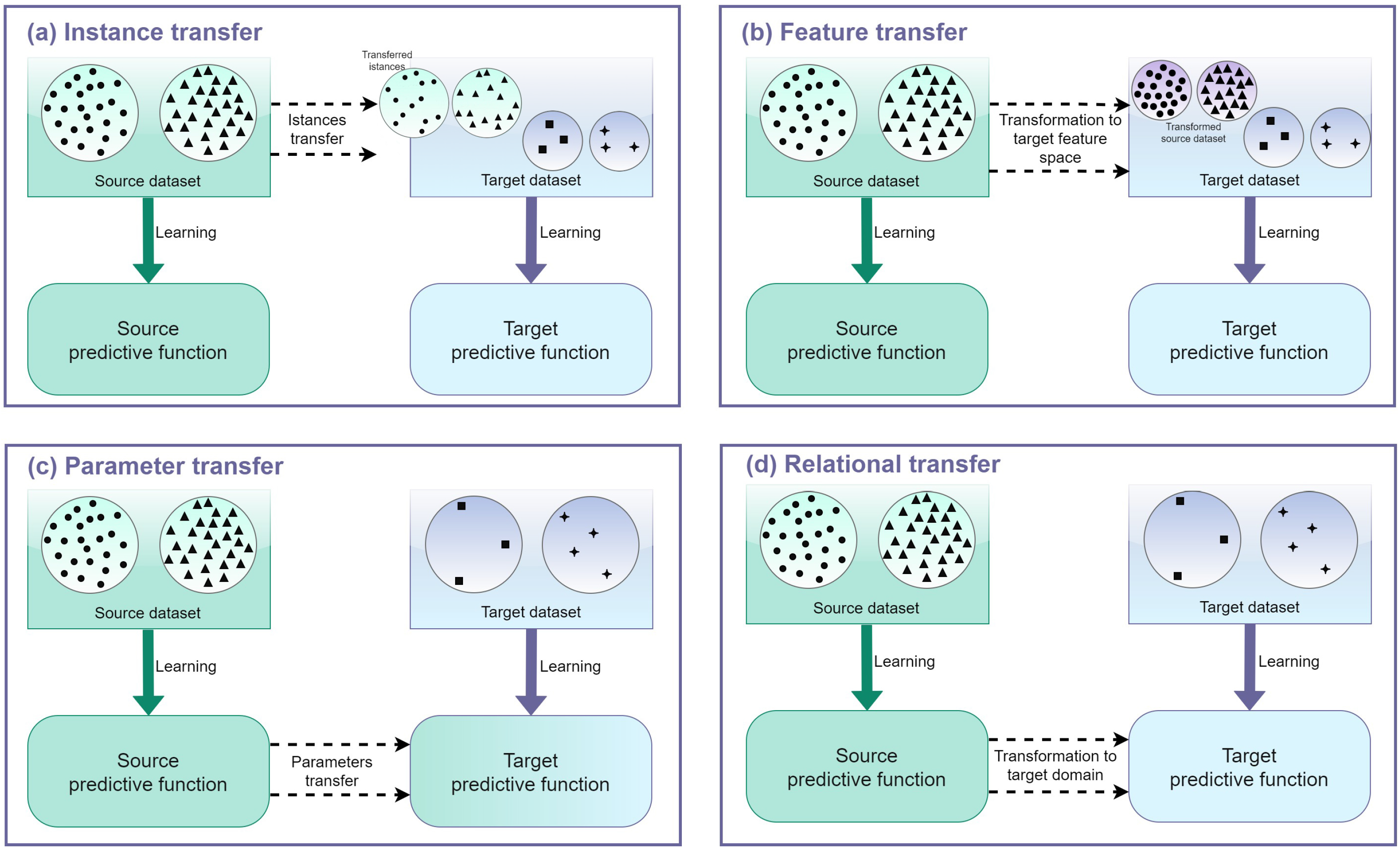
• Instance-based transfer: these approaches assume that due to the difference in distributions between the source and the target domains, certain parts of the data in the source domain can be reused, by reweighting them so as to reduce the effect of the “harmful” source data, while encouraging the “good” data;
• Feature-based transfer: the idea behind this approach is to learn a “good” feature representation for the target domain, to minimize the marginal and the conditional distribution differences, preserving the properties or the potential structures of the data, and classification or regression model error. For instance, a solution is to find the common latent features through feature transformation and use them as a bridge to transfer knowledge: this case is referred to as a symmetric feature-based transfer since both the source and the target features are transformed into a new feature representation; in contrast, in the asymmetric case, the source features are transformed to match the target ones. When performing feature transformation to reduce the distribution difference, one issue is how to measure such differences or similarities. This is done through specific ad-hoc metrics, which are described in Section 3.1;
• Parameter-based transfer: this approach performs the transfer at the model/parameter level by assuming that models for related tasks should share some parameters or prior distributions of hyperparameters. So, by discovering them, knowledge is transferred across tasks themselves;
• Relational-based transfer: these approaches deal with transfer learning for relational domains, where the data are non-independent and identically distributed (i.i.d.) and can be represented by multiple relations. The assumption is that some relationship among the data in the source and target domains is similar and that is the knowledge to be transferred, transferring the logical relationship or rules learned in the source domain to the target domain.

The references reported in this paper are classified based on the above categories. In the next section, some metrics generally used in the TL framework are briefly introduced.

3.1. Distribution Distance Metrics

Metrics to evaluate the differences among data distributions are commonly adopted in feature-based TL to learn a new space that reduces the difference of distribution between the two domains. How to measure the distribution difference or the similarity between domains is, therefore, an important task. They are used in instance-based TL methods as well to produce the weights of the instances by minimizing the adopted metric between the domains [40]. In

Table 2. Metrics commonly adopted in TL to quantify the distribution difference between datasets.

Distribution Difference Measure	Algorithm	Applications
Maximum Mean Discrepancy (MMD)	[41]	[42,43]
Kullback–Leibler Divergence ($D_{KL}$)	[44]	[45,46]
Jensen–Shannon Divergence (JSD)	[47]	[48,49]
Bregman Distance ($D_F$)	[50]	[51,52]
Hilbert–Schmidt Independence Criterion (HSIC)	[53]	[54,55]
Wasserstein Distance (W)	[56]	[57,58]
Central Moment Discrepancy (CMD)	[59]	[60,61]

the most adopted metrics in TL techniques are reported.

They are defined in the following.

• Maximum Mean Discrepancy (MMD) [41]
  Given two distributions P and Q, MMD is defined as the distance between the means of them mapped into a Reproducing Kernel Hilbert Space (RKHS):

  $$MMD(P,Q)=\Vert {\mu }_P-{\mu }_Q{\Vert }_{\mathcal{H}}.$$

  (11)

  where $\mu$ represents the mean value of the distribution.
  The MMD is one of the most used measures in TL. One known feature representation method for TL called Transfer Component Analysis (TCA) [42] learns some transfer components across domains in an RKHS using MMD. Another unsupervised feature transformation technique called Joint Distribution Adaptation (JDA) jointly adapts both the marginal and conditional distributions of the domains in a dimensionality reduction procedure based on Principal Component Analysis (PCA) and the MMD measure [43].
• Kullback–Leibler Divergence ($D_{KL}$) [44]
  $D_{KL}$ is an asymmetric measure of how one probability distribution differs from another. Given two discrete probability distributions, P and Q on the same probability space $\mathcal{X}$, $D_{KL}$, or the relative entropy, from Q to P is defined as:

  $$D_{KL}(P \Vert Q)=\sum _{x\in \mathcal{X}}P\left(x\right)log\left(\frac{P\left(x\right)}{Q\left(x\right)}\right).$$

  (12)
  In Zhuang et al. [45] a supervised representation learning method based on deep autoencoders for TL is introduced so that the distance in distributions of the instances between the source and the target domains is minimized in terms of $D_{KL}$. Feature-based TL realized through autoencoders is proposed in Guo et al. [46], where $D_{KL}$ is adopted to measure the similarity of new samples concerning historical data samples.
• Jensen–Shannon Divergence (JSD) [47,48,49]
  JSD is a symmetric and smooth version of $D_{KL}$, defined as:

  $$JSD(P \Vert Q)=\frac{1}{2}{D}_{KL}(P \Vert M)+\frac{1}{2}{D}_{KL}(Q \Vert M),$$

  (13)

  with M being $M=\frac{1}{2}(P+Q)$.
  JSD is used in Dey et al. [48] as a distance metric in a clustering technique for domain adaptation purposes. A classification method for TL proposed in Chen et al. [49] exploits the JSD measure with a PCA feature mapping technique.
• Bregman Distance ($D_F$) [50]
  $D_F$ is a difference measure between two points defined in terms of a strictly convex function called Bregman function F. The points can be interpreted as probability distributions. Given $F:\mathrm{\Omega }\to \mathbb{R}$ a continuously-differentiable, strictly convex function defined on a closed convex set $\mathrm{\Omega }$, the Bregman distance $D_F$ associated with F for points $p,q\in \mathrm{\Omega }$ is defined as the difference between the value of F at point p and the value of the first-order Taylor expansion of F around point q evaluated at point p:

  $$D_F(p,q)=F\left(p\right)-F\left(q\right)-\langle ▿F\left(q\right),p-q\rangle .$$

  (14)
  A TL method for hyperspectral image classification proposed in Shi et al. [51] employs a regularization based on $D_F$ to find common feature representation for both the source domain and target domain. A domain adaptation approach introduced in Sun et al. [52] reduces the discrepancy between the source domain and the target domain in a latent discriminative subspace by minimizing a $D_F$ matrix divergence function.
• Hilbert–Schmidt Independence Criterion (HSIC) [53]
  Given separable RKHSs $\mathcal{F}$, $\mathcal{G}$ and a joint measure $p_{xy}$ over $\left(\mathcal{X}\times \mathcal{Y},\mathrm{\Gamma }\times \mathrm{\Lambda }\right)$, HSIC is defined as the squared HS-norm of the associated cross-covariance operator $C_{xy}$:

  $$HSIC(p_{xy},\mathcal{F},\mathcal{G}):={\Vert C_{xy} \Vert }_{HS}^2.$$

  (15)
  A domain adaptation method called Maximum Independence Domain Adaptation (MIDA) finds a latent feature space in which the samples and their domain features are maximally independent in the sense of HSIC [54]. Another method to find the structural similarity between two source and target domains is proposed in Wang and Yang [55]. The algorithm extracts the structural features within each domain and then maps them into the RKHS. The dependencies estimations across domains are performed using the HSIC.
• Wasserstein Distance (W) [56]
  Given two distributions P and Q, the pth Wasserstein distance metric W is defined as:

  $$W:=W(F_P,F_Q)={\left({\int }_0^1\mid F_P^{-1}\left(u\right)-F_Q^{-1}\left(u\right){\mid }^{p}du\right)}^{\frac{1}{p}},$$

  (16)

  where $F_P$ and $F_Q$ are the corresponding cumulative distribution functions and $F_P^{-1}$ and $F_Q^{-1}$ the respective quantile functions.
  W is employed in Shen et al. [57] for an algorithm that aims to learn domain invariant feature representation. It utilizes an ANN to estimate the empirical W distance between the source and target samples and optimizes a feature extractor network to minimize the estimated W in an adversarial manner. A W-based asymmetric adversarial domain adaptation is proposed also in Ying et al. [58] for unsupervised domain adaptation for fault diagnosis.
• Central Moment Discrepancy (CMD) [59]
  CMD is a distance function on probability distributions on compact intervals. Given two bounded random vectors $X=(X_1,\dots ,X_N)$ and $Y=(Y_1,\dots ,Y_N)$ i.i.d. and two probability distributions P and Q on the compact interval ${[a,b]}^N$, CMD is defined as

  $$CMD(P,Q)=\frac{1}{\mid b-a\mid }{ \Vert \mathbb{E}\left(X\right)-\mathbb{E}\left(Y\right) \Vert }_2+\sum _{k=2}^{\infty }\frac{1}{{\mid b-a\mid }^k}{ \Vert c_k\left(X\right)-c_k\left(Y\right) \Vert }_2,$$

  (17)

  where $\mathbb{E}\left(X\right)$ is the expectation of X and $c_k\left(X\right)$ is the central moment vector of order k defined in Zellinger et al. [59].
  In a domain adaptation method for fault detection presented in Li et al. [60], a CNN is applied to extract features from two differently distributed domains and the distribution discrepancy is reduced using the CMD criterion. Another CNN- and CMD-based for fault detection is proposed in Xiong et al. [61].

Since it is often difficult to design metrics that are well-suited to the particular data and task of interest, an ML field called Distance Metric Learning (DML) aims at automatically constructing task-specific distance metrics from supervised data [62]. As an ML task, DML suffers the same problems described so far, requiring a large amount of label information. For this reason, TL methods have been extended to this sub-field as well, in what is called Transfer Metric Learning (TML) [62]. These fields fall out of the scope of this paper.

The metrics introduced so far are also adopted in some TL implementations for SS for both feature- and instance-based TL methods, as described in the next section.

4. Transfer Learning in SS Design

The implementations of TL on SSs from the literature here considered are categorized in

Table 3. TL classifications.

	Problem Categorization						Approach Categorization
	Use Case		Label Avail.		Feature Space		TL Approach				ML Technique
	Cross-Phase	Cross-Entity	Inductive	Transductive	Homogeneous	Heterogeneous	Instance	Feature	Parameter	Relational
Batch processes
[63]	•		•		•				•		PLS
[64,65,66,67]	•	•	•		•	•		•			PLS
[68]		•	•		•			•			PLS
Production processes
[36]	•		•		•		•		•		ANN
[69]	•		•	•	•			•			LSTM, XGBoost
Multi-grade chemical processes
[70,71]	•		•		•		•				ELM
[72]	•		•		•		•		•		GAN, ELM
Industrial process systems
[73]	•		•		•				•		ANN
[10]		•	•		•				•		LSTM, RNN
[74,75]	•			•	•				•		MW, JITL
[46]	•		•		•		•	•			GMVAE, JITL
[11,76]	•	•		•	•			•			DANN
[77]	•		•		•		•	•			PCA, ANN

. Because of a lack of comparability between the different scenarios and cases, listing and comparing results (in terms of final performance or implementation burden) is not feasible. In the following sub-sections, the different solutions applied in the field of SS modelling are illustrated.

To better highlight the motivation behind the application of TL in SSs, works are here classified based on the use case as proposed in Maschler and Weyrich [15] (see Figure 6).

The cases considered are the following:

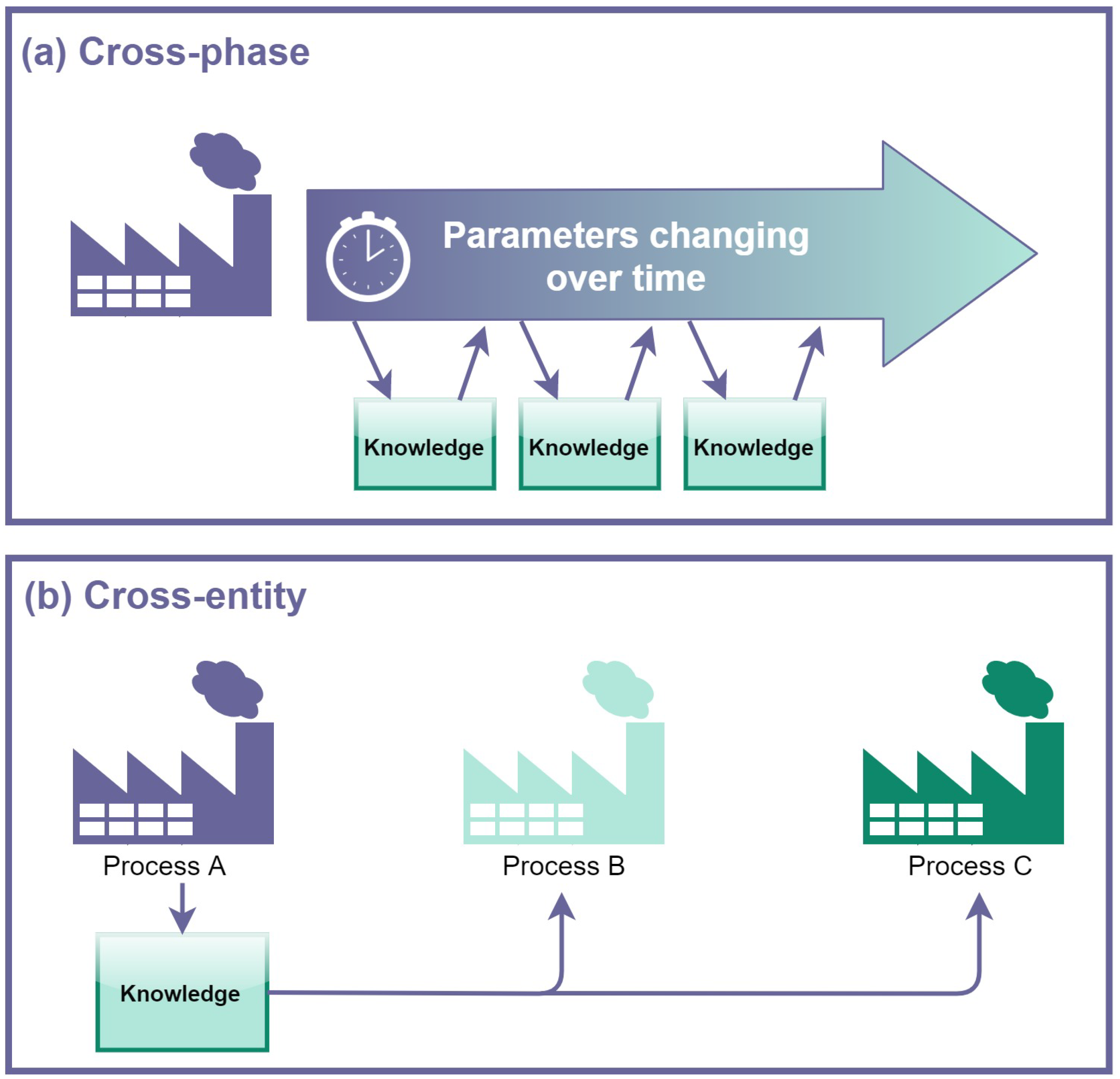
• Cross-phase, which is the case in which plants meet new working conditions and models lose accuracy: this can happen because of signal drift or different operative stages in multi-grade processes or, in the case of production processes, because of changes in products, tools, machines or materials;
• Cross-entity, which is the case in which TL is adopted to transfer knowledge between similar but physically different processes.

The classification is then performed from a problem and solution point of view: the former considers the TL settings described in Section 3, whereas in the latter the approach adopted and the chosen ML method are considered.

Finally, works are grouped into four groups based on the type of process, namely: batch processes, production processes, multi-grade chemical processes and industrial process systems.

4.1. Batch Processes

Industry processes in which the output appears in quantities of materials or lots and that present both characteristics of continuous and discrete processes are called batch processes. The product of a batch process is called a batch. Quality control of this kind of process is a difficult task due to nonlinearity and time variance. So, designing models able to capture accurately the process behaviour is a difficult task. One of the problems affecting batch process modelling is that sufficient data are often unavailable. The number of new batch data is indeed not sufficient to build a reliable process model. In Wang and Zhao [63], to solve this issue, a novel transfer and incremental SS is developed with the support of multiple historical process modes. The proposed algorithm, with the constant increase in new samples from the cloud of historical modes, can incrementally update model parameters to flexibly accommodate new process modes. To quantify the progressive prediction performance, the Root Mean Squared Error (RMSE) of eight different test batches is adopted. Prediction results of the proposed model are graphically compared with those of a general phase-based PLS (Partial Least Squares) model. The RMSE curve of the proposed model fluctuates around 0.05, whereas the one of the general model is high and unstable, revealing the goodness of the predictions of the real qualities of the product in the first case and the prediction inability of the general model.

The works [64,65,66,67] assess the problem of TL for batch processes for both the same process and for knowledge-transferring between similar processes as well. Similar batch processes employ the same or similar raw materials, equipment, and control strategies and the relationships between the process variables are the same or similar. One difficulty in applying TL in similar batch processes is that there are always differences between them, and this leads to a serious plant–model mismatch. The problem of applying TL in batch processes for quality prediction to solve both the problem of data scarcity and plant–model mismatch is assessed in these papers. The method proposed is based on the latent variable model (LVM) [78] and the joint-Y partial least squares (JY-PLS) regression [79]. The transferring of the process knowledge is achieved through a common latent variable space and the mismatch between variables is addressed through an adaptive control strategy. Results are evaluated in terms of RMSE between the proposed model and a Kernel-PLS (KPLS) model. The proposed model showed indeed a reduction in the RMSE of 56%.

The JY-PLS method is adopted also in Jia et al. [68] and the transferring method is based on domain-adaption between the source and target domains (DAJY-PLS). In particular, an index, which is the difference between the variance in source and target domains, is used to realize the trade-off between minimizing the difference of distributions, quantified through the MMD measure, of the domains and maximizing the covariance between the latent and output variables. The efficiency of the proposed approach is verified by comparing the DAJY-PLS and its JY-PLS counterpart, adopting RMSE and MAE (Mean Absolute Error) as a measure of performance. The DAJY-PLS showed an average reduction of 67% of the RMSE and of 68% in the MAE over ten different experiments.

4.2. Production Processes

Quality prediction is tackled in Tercan et al. [36] and Yao et al. [69] for production processes. Every time a change in production occurs, the process changes behavior, leading to the need for what is called incremental learning. In such a case, new target data are incrementally used to extend the source model’s knowledge. In Tercan et al. [36], an injection molding is considered. To assess the changes in the process behavior, an ANN is first trained on the source data and when the produced part is changed a new block of neurons, specially trained for the new part, is added, so that the model does not forget the knowledge from the previously learned parts. Such incremental learning approach is graphically compared, in terms of Correlation Coefficient (CC), to a baseline approach that does not adopt incremental learning but rather jointly trains the ANN on all data available to that point, when six different parts are produced. Results showed the incremental learning approach maintains a value of CC over 0.95 with every part, while the baseline approach cannot handle the increasing complexity in the data with an incremental drop in CC for every newly produced part.

In Yao et al. [69], quality prediction on cement clinker is performed through the prediction of the concentration of free calcium oxide (f-CaO). Incremental learning is needed because of the process time variance. A data-driven model based on deep dynamic features extracting and transferring methods is applied to build a SS for cement quality prediction. A large semi-supervised dataset is used to extract nonlinear dynamic features through a deep Long Short-Term Memory (LSTM) encoder–decoder network with an attention mechanism. The features are then transferred to an eXtreme Gradient Boosting (XGBoost) regression model for output prediction. The method is compared to other different models, both static and dynamic, for f-CaO content prediction proposed in other researches, in terms of CC and RMSE. In particular, the proposed method showed an improvement of the 285% of the CC and a reduction of 74% in the RMSE with respect to a simple static PLS model, whereas an improvement of 67% in the CC and a reduction of 65% in the RMSE with respect of a dynamic LSTM model.

4.3. Multi-Grade Chemical Processes

Multi-grade processes present multiple operating grades, each of them with an unknown distribution discrepancy of process data concerning the others. The same production line commonly produces different product grades after modifying the operating conditions and/or the ratio of ingredients in the process feed. Since key product qualities cannot be measured online and need laboratory analysis, manual operations for grade changeover are commonly implemented in practice, often leading to inefficient and off-grade products. The use of TL in such context allows application of the information from different grades to enlarge the prediction domain to some extent, even in the case of limited labeled samples.

In Yang et al. [70] and Liu et al. [71] the knowledge transfer between different grades is performed through an extension of Extreme Learning Machines (ELM), called Domain Adaptation ELM (DAELM). To implement the transfer, the empirical error from the target domain is used as a regularization term of the target-labeled instances. The DAELM method is compared to a regularized ELM (RELM) model over three grades, adopting each of them alternatively as a source domain in three different experiments. In particular, the method showed a reduction of 89% in the RMSE with the DAELM model when grade 3 data were used as source and grade 2 data as the target.

The method is further investigated in Liu et al. [72], where the distribution discrepancy between the grades is firstly reduced through a feature transformation using a GAN, before applying the DAELM method.

4.4. Industrial Process Systems

Signal drifts often affect process systems. These changes in data distribution over time lead to a decrease in SS performance.

In such cases, a possible solution for the designer is to fine-tune the model over the new working points. In Hsiao et al. [73], ANN fine-tuning strategies over small datasets are explored to adapt the SS of a refinery distillation column over time. To avoid losing previously learned knowledge the strategy adopted is to freeze the inner layers, updating only the outer ones. Performances are evaluated in terms of RMSE through graphical plots with respect to different-sized target data-sets, showing how the fine-tuned ANN performed better than its simple counterpart.

In Curreri et al. [10], fine-tuning and hyperparameter adaptation strategies are investigated in a cross-entity setting for different-sized target labeled datasets, in the design of a transferable SS for a Sulfur Recovery Unit (SRU). Experiments are performed using LSTMs and Recurrent Neural Networks (RNNs) to compare their transferability performance. To evaluate the performances of the proposed cross-entity method, results were compared between an optimized SS whose design procedure took 100 h and a transferred one whose transferring procedure took 7 min. In particular, RNN-based transferred SS showed an average degradation of only 8% of the CC on test data, whereas the LSTM-based transferred SS showed the same CC as the originally optimized one.

Some modelling methods are known to be effective against gradual and abrupt–recurrent changes in process characteristics, such as Moving Window (MW) and Just-In-Time-Learning (JITL). These two methods are adopted in Alakent [74], Alakent [75] where an adaptive learning frame to develop an SS able to contrast the signal drift phenomenon is proposed. The proposed method retunes the hyperparameters of the algorithm using a historical dataset through a weighting user-controlled parameter, which represents the trade-off between the information extracted from the new target samples and the JITL predictions. The technique is tested for the SS design of a debutanizer column (DC) and an SRU. The accuracy of the method is evaluated through the average RMSE for the studied cases. In the case of the DC, the transferring procedure reduced the RMSE by 66%, whereas in the case of the SRU, the RMSE was reduced by 31% for the first output and 23% for the second output.

A JITL-based model is used again in Guo et al. [46] where the transfer is performed through a feature extraction using a Gaussian Mixture Variational Autoencoder (GMVAE). When a new sample is considered, $D_{KL}$ is adopted to measure its similarity with historical data samples. Based on the result, weighted input and output historical data are obtained and used in the final model. Validation of the method is performed through RMSE, MAE and Mean Relative Error (MRE) between different JITL-based models from the literature and the proposed one. In particular, results on the adopted dataset showed a reduction of 48% in the RMSE and of 60% in the MAE and MRE with respect to a distance-based JITL model.

Feature-based knowledge transfer methods are investigated, in both cross-phase and cross-entity settings, as shown in Farahani et al. [11], Farahani et al. [76] for power plant SS design. A Domain Adversarial training Neural Network (DANN) approach is employed to firstly perform feature extraction and then the actual regression. In particular, the architecture of the DANN consists of three parts: a feature extractor, a regression model and a domain discriminator. The first maps m-dimensional input data into a one-dimensional feature representation. The second maps the latter into the output space, performing the prediction regression task. At the same time, the one-dimensional feature representation is introduced to the domain discriminator as well, which detects whether the input instances come from the source or target domain. To reduce the difference between the samples, the adversarial training procedure between the feature extractor and the domain discriminator is performed so that the extracted features become more indistinguishable between source and target domains. This way, the regression part, trained solely on the source data, can predict target data more accurately, without even needing their corresponding label. To quantify the performance of the performance of the $TL$, an index score here called $TransferRatio$ ($TR$) is introduced. TR is the target Mean Squared Error ($MSE$) when not using $TL$ over the target $MSE$ when using this $TL$ technique:

$$TransferRatio=\frac{TargetMSEwithoutTL}{TargetMSEwithTL}.$$

(18)

Results showed an average $TR$ of 2.93 between the studied cases in the cross-entity case and an average $TR$ of 1.81 between the studied cases in the cross-phase case.

Besides signal drifts, one of the problems afflicting SS design is labeled data scarcity, since process variables are sampled at a higher sample rate than quality variables. Incremental learning techniques to improve the performance of an SS when a low number of labeled data in the target domain are available is reported in Graziani and Xibilia [77]. The performance of an ANN-based SS for a refinery Sour Water Stripping (SWS) plant is improved by combining a preliminary PCA phase and a data selection procedure, based on DUPLEX and SPXY data selection algorithms. Evaluation of the approach is made in terms of CC and RMSE between the cases of simply applying a random-selection procedure without PCA and either DUPLEX and SPXY algorithms with PCA. Results showed an average improvement of 13% in the CC and a reduction of 14% of the RMSE in the case of PCA + DUPLEX with respect to the simple random-selection procedure.

5. Conclusions and Future Trends

The functionality of TL methods for SS design in industrial processes is a growing field of research. The existing literature demonstrates that TL can significantly enhance the SS performance, designing SSs that can both face cross-phase and cross-entity scenarios. Many questions are still open and need further research to make TL an efficient solution in industrial environments.

The first issue consists of a proper strategy to select the best transfer methods based on the process and dataset characteristics. The second issue refers to the definition of suitable metrics which allows evaluation of the applicability of each method providing an estimation of the transfer procedure performance. Another issue is related to determining the minimum size of the target dataset, both as regards input and output variables that guarantee the applicability of a given method. This should however depend both on the process characteristics and the applied method. Moreover, most of the implemented methods are actually parameter- and feature-based in homogeneous settings. Instance-based methods and heterogeneous settings, as well as relational-based approaches, still need further investigations.

The current applications and methods are still limited; further research is therefore needed also to evaluate the benefits of TL and compare the different strategies on real-world case studies. Hybrid solutions could be also investigated in the future to merge the advantages of different methods.

References

- Shardt, Y.A.; Yang, X.; Brooks, K.; Torgashov, A. Data Quality Assessment for System Identification in the Age of Big Data and Industry 4.0. IFAC-PapersOnLine 2020, 53, 104–113. [Google Scholar] [CrossRef]
- Fortuna, L.; Graziani, S.; Rizzo, A.; Xibilia, M.G. Soft Sensors for Monitoring and Control of Industrial Processes; Springer: London, UK, 2007; Volume 22. [Google Scholar]
- Kadlec, P.; Gabrys, B.; Strandt, S. Data-driven soft sensors in the process industry. Comput. Chem. Eng. 2009, 33, 795–814. [Google Scholar] [CrossRef] [Green Version]
- Graziani, S.; Xibilia, M.G. Deep learning for soft sensor design. In Development and Analysis of Deep Learning Architectures; Springer: Cham, Switzerland, 2020; pp. 31–59. [Google Scholar]
- Ben-David, S.; Blitzer, J.; Crammer, K.; Kulesza, A.; Pereira, F.; Vaughan, J.W. A theory of learning from different domains. Mach. Learn. 2010, 79, 151–175. [Google Scholar] [CrossRef] [Green Version]
- Murphy, K.P. Machine Learning: A Probabilistic Perspective; MIT Press: Cambridge, MA, USA, 2012. [Google Scholar]
- Kadlec, P.; Grbić, R.; Gabrys, B. Review of adaptation mechanisms for data-driven soft sensors. Comput. Chem. Eng. 2011, 35, 1–24. [Google Scholar] [CrossRef]
- Yang, B.; Lei, Y.; Jia, F.; Xing, S. An intelligent fault diagnosis approach based on transfer learning from laboratory bearings to locomotive bearings. Mech. Syst. Signal Process. 2019, 122, 692–706. [Google Scholar] [CrossRef]
- Pan, S.J.; Yang, Q. A survey on transfer learning. IEEE Trans. Knowl. Data Eng. 2009, 22, 1345–1359. [Google Scholar] [CrossRef]
- Curreri, F.; Patanè, L.; Xibilia, M.G. RNN- and LSTM-Based Soft Sensors Transferability for an Industrial Process. Sensors 2021, 21, 823. [Google Scholar] [CrossRef] [PubMed]
- Farahani, H.S.; Fatehi, A.; Nadali, A.; Shoorehdeli, M.A. A Novel Method For Designing Transferable Soft Sensors And Its Application. arXiv 2020, arXiv:2008.02186. [Google Scholar]
- Raghu, M.; Zhang, C.; Kleinberg, J.; Bengio, S. Transfusion: Understanding transfer learning for medical imaging. arXiv 2019, arXiv:1902.07208. [Google Scholar]
- Alibadi, Z.; Vidal, J.M. To Read or To Do? That’s The Task: Using Transfer Learning to Detect the Intent of an Email. In Proceedings of the 2018 International Conference on Computational Science and Computational Intelligence (CSCI), Las Vegas, NV, USA, 12–14 December 2018; pp. 1105–1110. [Google Scholar]
- Wang, D.; Zheng, T.F. Transfer learning for speech and language processing. In Proceedings of the 2015 Asia-Pacific Signal and Information Processing Association Annual Summit and Conference (APSIPA), Hong Kong, China, 16–19 December 2015; pp. 1225–1237. [Google Scholar]
- Maschler, B.; Weyrich, M. Deep transfer learning for industrial automation. IEEE Ind. Electron. Mag. 2021, 15, 65–75. [Google Scholar] [CrossRef]
- Fortuna, L.; Graziani, S.; Xibilia, M.G. Virtual instruments in refineries. IEEE Instrum. Meas. Mag. 2005, 8, 26–34. [Google Scholar] [CrossRef]
- Curreri, F.; Graziani, S.; Xibilia, M.G. Input selection methods for data-driven Soft sensors design: Application to an industrial process. Inf. Sci. 2020, 537, 1–17. [Google Scholar] [CrossRef]
- Patanè, L.; Xibilia, M.G. Echo-state networks for soft sensor design in an SRU process. Inf. Sci. 2021, 566, 195–214. [Google Scholar] [CrossRef]
- Graziani, S.; Xibilia, M.G. Deep structures for a reformer unit soft sensor. In Proceedings of the 2018 IEEE 16th International Conference on Industrial Informatics (INDIN), Porto, Portugal, 18–20 July 2018; pp. 927–932. [Google Scholar]
- Stanišić, D.; Jorgovanović, N.; Popov, N.; Čongradac, V. Soft sensor for real-time cement fineness estimation. ISA Trans. 2015, 55, 250–259. [Google Scholar] [CrossRef]
- Sujatha, K.; Bhavani, N.P.; Cao, S.Q.; Kumar, K.R. Soft Sensor for Flame Temperature Measurement and IoT based Monitoring in Power Plants. Mater. Today Proc. 2018, 5, 10755–10762. [Google Scholar] [CrossRef]
- Galicia, H.J.; He, Q.P.; Wang, J. A reduced order soft sensor approach and its application to a continuous digester. J. Process Control 2011, 21, 489–500. [Google Scholar] [CrossRef]
- Zhu, X.; Rehman, K.U.; Wang, B.; Shahzad, M. Modern soft-sensing modeling methods for fermentation processes. Sensors 2020, 20, 1771. [Google Scholar] [CrossRef] [Green Version]
- Zhu, C.H.; Zhang, J. Developing soft sensors for polymer melt index in an industrial polymerization process using deep belief networks. Int. J. Autom. Comput. 2020, 17, 44–54. [Google Scholar] [CrossRef] [Green Version]
- Pisa, I.; Santín, I.; Vicario, J.L.; Morell, A.; Vilanova, R. ANN-based soft sensor to predict effluent violations in wastewater treatment plants. Sensors 2019, 19, 1280. [Google Scholar] [CrossRef] [Green Version]
- Souza, F.A.; Araújo, R.; Mendes, J. Review of soft sensor methods for regression applications. Chemom. Intell. Lab. Syst. 2016, 152, 69–79. [Google Scholar] [CrossRef]
- Bishop, C.M. Pattern Recognition and Machine Learning. Mach. Learn. 2006, 128, 738. [Google Scholar]
- Ljung, L. System identification. In Signal Analysis and Prediction; Birkhäuser: Boston, MA, USA, 1998; pp. 163–173. [Google Scholar]
- Curreri, F.; Fiumara, G.; Xibilia, M.G. Input selection methods for soft sensor design: A survey. Future Internet 2020, 12, 97. [Google Scholar] [CrossRef]
- Pani, A.K.; Amin, K.G.; Mohanta, H.K. Soft sensing of product quality in the debutanizer column with principal component analysis and feed-forward artificial neural network. Alex. Eng. J. 2016, 55, 1667–1674. [Google Scholar] [CrossRef] [Green Version]
- Wang, K.; Shang, C.; Liu, L.; Jiang, Y.; Huang, D.; Yang, F. Dynamic soft sensor development based on convolutional neural networks. Ind. Eng. Chem. Res. 2019, 58, 11521–11531. [Google Scholar] [CrossRef]
- Wang, X. Data Preprocessing for Soft Sensor Using Generative Adversarial Networks. In Proceedings of the 2018 15th International Conference on Control, Automation, Robotics and Vision (ICARCV), Singapore, 18–21 November 2018; pp. 1355–1360. [Google Scholar]
- Liu, R.; Rong, Z.; Jiang, B.; Pang, Z.; Tang, C. Soft Sensor of 4-CBA Concentration Using Deep Belief Networks with Continuous Restricted Boltzmann Machine. In Proceedings of the 2018 5th IEEE International Conference on Cloud Computing and Intelligence Systems (CCIS), Nanjing, China, 23–25 November 2018; pp. 421–424. [Google Scholar]
- Chitralekha, S.B.; Shah, S.L. Support Vector Regression for soft sensor design of nonlinear processes. In Proceedings of the 18th Mediterranean Conference on Control and Automation (MED’10), Marrakech, Morocco, 23–25 June 2010; pp. 569–574. [Google Scholar]
- Grbić, R.; Slišković, D.; Kadlec, P. Adaptive soft sensor for online prediction and process monitoring based on a mixture of Gaussian process models. Comput. Chem. Eng. 2013, 58, 84–97. [Google Scholar] [CrossRef]
- Tercan, H.; Guajardo, A.; Meisen, T. Industrial Transfer Learning: Boosting Machine Learning in Production. In Proceedings of the 2019 IEEE 17th International Conference on Industrial Informatics (INDIN), Helsinki, Finland, 22–25 July 2019; Volume 1, pp. 274–279. [Google Scholar]
- Blitzer, J.; Dredze, M.; Pereira, F. Biographies, bollywood, boom-boxes and blenders: Domain adaptation for sentiment classification. In Proceedings of the 45th Annual Meeting of the Association of Computational Linguistics, Prague, Czech Republic, 24–29 June 2007; pp. 440–447. [Google Scholar]
- Wang, Z.; Dai, Z.; Póczos, B.; Carbonell, J. Characterizing and avoiding negative transfer. In Proceedings of the IEEE/CVF Conference on Computer Vision and Pattern Recognition, Long Beach, CA, USA, 15–20 June 2019; pp. 11293–11302. [Google Scholar]
- Redko, I.; Morvant, E.; Habrard, A.; Sebban, M.; Bennani, Y. Advances in Domain Adaptation Theory; Elsevier: Amsterdam, The Netherlands, 2019. [Google Scholar]
- Huang, J.; Gretton, A.; Borgwardt, K.; Schölkopf, B.; Smola, A. Correcting sample selection bias by unlabeled data. Adv. Neural Inf. Process. Syst. 2006, 19, 601–608. [Google Scholar]
- Borgwardt, K.M.; Gretton, A.; Rasch, M.J.; Kriegel, H.P.; Schölkopf, B.; Smola, A.J. Integrating structured biological data by kernel maximum mean discrepancy. Bioinformatics 2006, 22, e49–e57. [Google Scholar] [CrossRef] [Green Version]
- Pan, S.J.; Tsang, I.W.; Kwok, J.T.; Yang, Q. Domain adaptation via transfer component analysis. IEEE Trans. Neural Netw. 2010, 22, 199–210. [Google Scholar] [CrossRef] [PubMed] [Green Version]
- Long, M.; Wang, J.; Ding, G.; Sun, J.; Yu, P.S. Transfer feature learning with joint distribution adaptation. In Proceedings of the IEEE International Conference on Computer Vision, Sydney, Australia, 1–8 December 2013; pp. 2200–2207. [Google Scholar]
- Kullback, S.; Leibler, R.A. On information and sufficiency. Ann. Math. Stat. 1951, 22, 79–86. [Google Scholar] [CrossRef]
- Zhuang, F.; Cheng, X.; Luo, P.; Pan, S.J.; He, Q. Supervised representation learning: Transfer learning with deep autoencoders. In Proceedings of the Twenty-Fourth International Joint Conference on Artificial Intelligence, Buenos Aires, Argentina, 25–31 July 2015. [Google Scholar]
- Guo, F.; Wei, B.; Huang, B. A just-in-time modeling approach for multimode soft sensor based on Gaussian mixture variational autoencoder. Comput. Chem. Eng. 2021, 146, 107230. [Google Scholar] [CrossRef]
- Endres, D.M.; Schindelin, J.E. A new metric for probability distributions. IEEE Trans. Inf. Theory 2003, 49, 1858–1860. [Google Scholar] [CrossRef] [Green Version]
- Dey, S.; Madikeri, S.; Motlicek, P. Information theoretic clustering for unsupervised domain-adaptation. In Proceedings of the 2016 IEEE International Conference on Acoustics, Speech and Signal Processing (ICASSP), Shanghai, China, 20–25 March 2016; pp. 5580–5584. [Google Scholar]
- Chen, W.H.; Cho, P.C.; Jiang, Y.L. Activity recognition using transfer learning. Sens. Mater 2017, 29, 897–904. [Google Scholar]
- Bregman, L.M. The relaxation method of finding the common point of convex sets and its application to the solution of problems in convex programming. USSR Comput. Math. Math. Phys. 1967, 7, 200–217. [Google Scholar] [CrossRef]
- Shi, Q.; Zhang, Y.; Liu, X.; Zhao, K. Regularised transfer learning for hyperspectral image classification. IET Comput. Vis. 2019, 13, 188–193. [Google Scholar] [CrossRef]
- Sun, H.; Liu, S.; Zhou, S. Discriminative subspace alignment for unsupervised visual domain adaptation. Neural Process. Lett. 2016, 44, 779–793. [Google Scholar] [CrossRef]
- Gretton, A.; Fukumizu, K.; Teo, C.H.; Song, L.; Schölkopf, B.; Smola, A.J. A kernel statistical test of independence. In Proceedings of the Twenty-First Annual Conference on Neural Information Processing Systems, Vancouver, BC, Canada, 3–6 December 2007; Volume 20, pp. 585–592. [Google Scholar]
- Yan, K.; Kou, L.; Zhang, D. Learning domain-invariant subspace using domain features and independence maximization. IEEE Trans. Cybern. 2017, 48, 288–299. [Google Scholar] [CrossRef] [Green Version]
- Wang, H.; Yang, Q. Transfer learning by structural analogy. In Proceedings of the Twenty-Fifth AAAI Conference on Artificial Intelligence, San Francisco, CA, USA, 7–11 August 2011. [Google Scholar]
- Vaserstein, L.N. Markov processes over denumerable products of spaces, describing large systems of automata. Probl. Peredachi Informatsii 1969, 5, 64–72. [Google Scholar]
- Shen, J.; Qu, Y.; Zhang, W.; Yu, Y. Wasserstein distance guided representation learning for domain adaptation. In Proceedings of the Thirty-Second AAAI Conference on Artificial Intelligence, New Orleans, LA, USA, 2–7 February 2018. [Google Scholar]
- Ying, Y.; Jun, Z.; Tang, T.; Jingwei, W.; Ming, C.; Jie, W.; Liang, W. Wasserstein distance based Asymmetric Adversarial Domain Adaptation in intelligent bearing fault diagnosis. Meas. Sci. Technol. 2021, 32, 115019. [Google Scholar]
- Zellinger, W.; Grubinger, T.; Lughofer, E.; Natschläger, T.; Saminger-Platz, S. Central moment discrepancy (cmd) for domain-invariant representation learning. arXiv 2017, arXiv:1702.08811. [Google Scholar]
- Li, X.; Hu, Y.; Zheng, J.; Li, M.; Ma, W. Central moment discrepancy based domain adaptation for intelligent bearing fault diagnosis. Neurocomputing 2021, 429, 12–24. [Google Scholar] [CrossRef]
- Xiong, P.; Tang, B.; Deng, L.; Zhao, M.; Yu, X. Multi-block domain adaptation with central moment discrepancy for fault diagnosis. Measurement 2021, 169, 108516. [Google Scholar] [CrossRef]
- Pan, J. Review of metric learning with transfer learning. AIP Conf. Proc. 2017, 1864, 020040. [Google Scholar]
- Wang, J.; Zhao, C. Mode-cloud data analytics based transfer learning for soft sensor of manufacturing industry with incremental learning ability. Control Eng. Pract. 2020, 98, 104392. [Google Scholar] [CrossRef]
- Chu, F.; Shen, J.; Dai, W.; Jia, R.; Ma, X.; Wang, F. A dual modifier adaptation optimization strategy based on process transfer model for new batch process. IFAC-PapersOnLine 2018, 51, 791–796. [Google Scholar] [CrossRef]
- Chu, F.; Zhao, X.; Yao, Y.; Chen, T.; Wang, F. Transfer learning for batch process optimal control using LV-PTM and adaptive control strategy. J. Process Control 2019, 81, 197–208. [Google Scholar] [CrossRef]
- Chu, F.; Wang, J.; Zhao, X.; Zhang, S.; Chen, T.; Jia, R.; Xiong, G. Transfer learning for nonlinear batch process operation optimization. J. Process Control 2021, 101, 11–23. [Google Scholar] [CrossRef]
- Chu, F.; Cheng, X.; Peng, C.; Jia, R.; Chen, T.; Wei, Q. A process transfer model-based optimal compensation control strategy for batch process using just-in-time learning and trust region method. J. Frankl. Inst. 2021, 358, 606–632. [Google Scholar] [CrossRef]
- Jia, R.; Zhang, S.; You, F. Transfer learning for end-product quality prediction of batch processes using domain-adaption joint-Y PLS. Comput. Chem. Eng. 2020, 140, 106943. [Google Scholar] [CrossRef]
- Yao, L.; Jiang, X.; Huang, G.; Qian, J.; Shen, B.; Xu, L.; Ge, Z. Virtual Sensing f-CaO Content of Cement Clinker Based on Incremental Deep Dynamic Features Extracting and Transferring Model. IEEE Trans. Instrum. Meas. 2020, 70, 1–10. [Google Scholar]
- Yang, C.; Chen, B.; Wang, Z.; Yao, Y.; Liu, Y. Transfer learning soft sensor for product quality prediction in multi-grade processes. In Proceedings of the 2019 IEEE 8th Data Driven Control and Learning Systems Conference (DDCLS), Dali, China, 24–27 May 2019; pp. 1148–1153. [Google Scholar]
- Liu, Y.; Yang, C.; Liu, K.; Chen, B.; Yao, Y. Domain adaptation transfer learning soft sensor for product quality prediction. Chemom. Intell. Lab. Syst. 2019, 192, 103813. [Google Scholar] [CrossRef]
- Liu, Y.; Yang, C.; Zhang, M.; Dai, Y.; Yao, Y. Development of adversarial transfer learning soft sensor for multigrade processes. Ind. Eng. Chem. Res. 2020, 59, 16330–16345. [Google Scholar] [CrossRef]
- Hsiao, Y.D.; Kang, J.L.; Wong, D.S.H. Development of Robust and Physically Interpretable Soft Sensor for Industrial Distillation Column Using Transfer Learning with Small Datasets. Processes 2021, 9, 667. [Google Scholar] [CrossRef]
- Alakent, B. Soft sensor design using transductive moving window learner. Comput. Chem. Eng. 2020, 140, 106941. [Google Scholar] [CrossRef]
- Alakent, B. Soft-sensor design via task transferred just-in-time-learning coupled transductive moving window learner. J. Process Control 2021, 101, 52–67. [Google Scholar]
- Farahani, H.S.; Fatehi, A.; Nadali, A.; Shoorehdeli, M.A. Domain Adversarial Neural Network Regression to design transferable soft sensor in a power plant. Comput. Ind. 2021, 132, 103489. [Google Scholar] [CrossRef]
- Graziani, S.; Xibilia, M.G. Improving Soft Sensors performance in the presence of small datasets by data selection. In Proceedings of the 2020 IEEE International Instrumentation and Measurement Technology Conference (I2MTC), Dubrovnik, Croatia, 25–28 May 2020; pp. 1–6. [Google Scholar]
- Jaeckle, C.M.; MacGregor, J.F. Product transfer between plants using historical process data. AIChE J. 2000, 46, 1989–1997. [Google Scholar] [CrossRef]
- Muñoz, S.G.; MacGregor, J.F.; Kourti, T. Product transfer between sites using Joint-Y PLS. Chemom. Intell. Lab. Syst. 2005, 79, 101–114. [Google Scholar]