Dynamic, Adaptive Inline Process Monitoring for Laser Material Processing by Means of Low Coherence Interferometry

Abstract

Surface laser structuring of electrical steel sheets can be used to manipulate their magnetic properties, such as energy losses and contribute to a more efficient use. This requires a technology such as low coherence interferometry, which makes it possible to be coupled directly into the existing beam path of the process laser and enables the possibility for an 100% inspection during the process. It opens the possibility of measuring directly in the machine, without removing the workpiece, as well as during the machining process. One of the biggest challenges in integrating an LCI measurement system into an existing machine is the need to use a different wavelength than the one for which the optical components were designed. This results in an offset between the measurement and processing spot. By integrating an additional scanning system exclusively for the measuring beam and developing a compensation model for the non-linear spot offset, this can be adaptively corrected by up to 98.9% so that the ablation point can be measured. The simulation model can also be easily applied to other systems with different components and at the same time allows further options for in-line quality assurance.

1. Introduction

Saving energy is becoming increasingly important. Especially in the area of generation and transformation of electrical energy, a considerable loss is to be expected. In the case of classic electrical sheet, several layers of steel and insulation materials are stacked. Electrical steel is used in a wide range of applications, from transformers and sensors to motors and generators [1,2,3,4]. One of the most important aspects of electric steel is the energy density. Unfortunately, a high energy density also leads to an increased energy loss. At the same time, noise generation is also increased due to, among other things, long-term delamination of the steel stack [5,6,7].

One way to improve these factors is to laser-texture the steel sheets. Laser micro structuring is an excellent solution due to its capacity to create functional surface structures on a micrometer scale [8,9,10,11,12,13,14,15]. The aim of the Horizon 2020 research project ESSIAL is, among other things, to improve the magnetic properties, as described above, by laser structuring of the steel sheets. The structures being considered are on grain-oriented (GO) electrical steel with the spatially width in the range of 25–500 µm and 1–25 µm depth range, as well as structures on grain non-oriented (GNO) in the range of 10–25 µm in width and 1–50 µm in depth [16,17,18].

To ensure that the target parameters of the process are met, a monitoring system is required that also minimizes the influence on the process and the machine itself and can be used to constantly observe the process and to avoid production rejects and to make production even more resource-efficient [19,20]. The low coherence interferometry (LCI) allows here the measurement of the ablation and thus the over surface structures without the need to remove the workpiece from the machine and at the same time uses the same beam path as the existing laser structuring process. LCI is an extension of classical optical coherence tomography (OCT) [21]. OCT was developed for ophthalmology in the early 1990s and has already been used in technical applications for several years [22,23,24,25,26]. While OCT provides high resolution imaging results for tomographic images, using the LCI method allows the measurement of the surface distance and thus the derivation of the topology of the surface on the workpiece [27,28]. The optical components of a laser machine are designed for a specific wavelength range, and the wavelength of the process laser is located in this range. The energy of the process laser is capable of destroying the components of the measuring system, so that the two systems must be separated in a certain way. A beam splitter can be used to achieve this, but the measurement wavelength must still be different from the wavelength of the process laser. This results in a non-linear offset between the spot positions of the two beams, so that simultaneous measurement and processing of the same position is no longer possible. The distance between the two spots increases as the beam moves further away from the center of the objective lens. In principle, this can be compensated by a color-corrected objective lens, but not completely or the choice of these objectives are very limited [29,30]. For this to be done, it is necessary to develop a method that allows this non-linear offset to be compensated adaptively during the process, thus allowing direct measurement of the material ablation. It must also be investigated how such compensation can be implemented and controlled.

The strategy and the development of a system that meets these requirements is described in the following sections. The goal of the ESSIAL research project is to integrate a measuring system into the laser process. For this purpose, a laboratory system will be developed and then scaled up step by step to complete machine integration. In this paper the focus is on the compensation of the spot offset caused by the different wavelengths between the processing laser and the measuring system. In this way, a measuring system is developed that enables 100% quality control while enabling use on an industrial scale.

2. Measuring Principle

The measuring principle of the LCI is based on the interferometric evaluation of the change in optical path length. One big advantage of the LCI method is the independence between axial resolution ${\sigma }_z$ and lateral resolution ${\sigma }_{\left(x,y\right)}$. While the axial resolution and the axial measuring range depends on the used light source, shown in Equations (1) and (2), the used scanning lens and scanning system have a big impact on the lateral resolution, shown in Equation (3) [22].

Assuming a Gaussian beam axial resolution and range and lateral resolution are defined by:

$${\sigma }_z=\frac{2\ln 2}{\pi }\frac{{\lambda }_0^2}{\Delta \lambda },$$

(1)

$${\mathsf{\Delta }}_z=\frac{N}{4n}\frac{{\lambda }_0^2}{\mathsf{\Delta }\lambda },$$

(2)

$${\sigma }_{x,y}=\frac{\mathsf{\Delta }\lambda }{\pi }\frac{f}{d},$$

(3)

where $\mathsf{\Delta }\lambda$ is the spectral width and ${\lambda }_0$ the central wavelength of the light source, n the average refractive index of the sample, N is the number of used pixels of the detector, d is the beam diameter at objective lens entry and f is the focal length of the used objective lens [29,31]. A nomenclature of the dimensions and quantities used can be found in the Appendix A.

3. Development of a Laboratory Setup

The challenges of integrating a measurement system into an existing beam path are complex. Different wavelengths must be used so that a separation can be made between the measuring system and the process laser. At the same time, the optics used are designed only for the process laser, so that strong chromatic aberrations must be expected here [28]. Thus, a suitable choice of the measuring wavelength is no longer trivial. An ultra-short pulse laser (USP) with a central wavelength of 1030 nm is used for the machining process. The laser has a pulse width of 500 fs and a pulse frequency of 10 kHz.

Based on the parameters of the laser, the scanner and the optics used, the central wavelength of the LCI measurement system can now be determined. For this purpose, different potential wavelengths were first tested by means of an optical simulation with the replica of the machine’s beam path. At the same time, one of the most important components is the beam splitter, which is intended to separate the two beams. Since the beam path is optimized for a wavelength of 1030 nm, the wavelength of the measuring system should be as close to this as possible. As shown in Equation (2), a high spectral width of the light source is advantageous. To take these boundary conditions into account, a beam splitter with a steep slope is necessary.

The combination of the NFD01–1040 beam splitter from Semrock and the Superlum SLD-471UBB was identified as the optimum combination, see Figure 1. In the use case considered here, the smallest structure is at a depth of 1 µm, so that the resolution of the measuring system must cover this. Equation (1) shows a theoretical axial resolution of 3.632 µm for the light source used with a central wavelength of 930 nm and a FWHM of 115 nm. It indicates the ability of the system to differentiate between different layers tomographically, but here a topographic measurement is made. For topographic evaluations, the repeatability must be taken into account, which is 0.36 µm, as will be shown later. Therefore, all structures of the use case can be resolved. To ensure optimal utilization of the broadband light, a suitable spectrometer is required that can capture the entire spectral width.

3.1. Development of the Spectrometer

The spectrometer is one of the central components of the SD-LCI. In the spectrometer, the superimposed signals from the measuring and reference arms are broken down into their spectral components and evaluated. It consists of an optical grating to diffract the radiation, a lens package to focus the diffracted spectrum and the camera on whose line the focus is set. Simulations were used to determine the lens package in the spectrometer. The aim of the simulation is to image the measurement spectrum on the camera line with the smallest possible spot sizes, taking into account all pixels of the camera as well as the entire wavelength range of the light source.

To avoid a loss of intensity, the beam diameter used to illuminate the grating was chosen to be 10 mm. This ensures that the light does not come into contact with the non-optical components of the spectrometer. Initially, some lens configurations were simulated with an automated simulation; for cost reasons, only standard lenses were used.

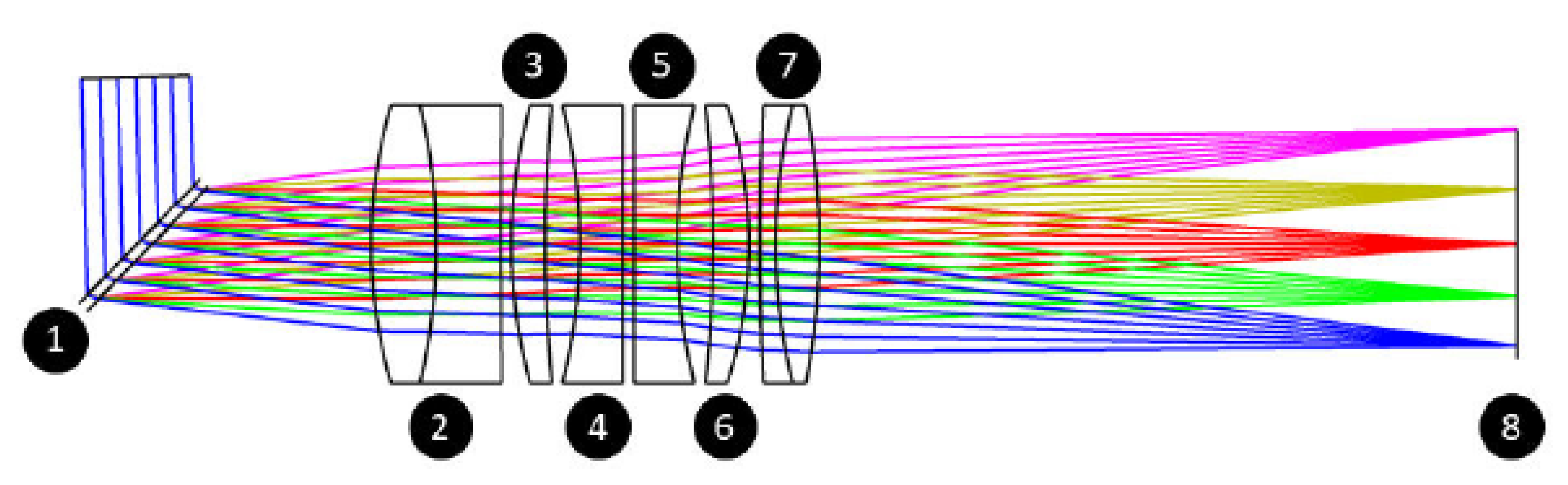
The three best configurations were then further optimized manually. The parameters considered here were the size of the Airy-disc, the diffraction limit and the RMS of the spot radii. In a further step, the behaviour of the systems was compared with the MTF to achieve an optimal contrast ratio. Figure 2 shows a schematic sketch of the optical components of the optimized system.

Based on the simulation with Zemax, a system for beam shaping within the spectrometer could be identified and already optically designed. Thereby the boundary conditions for the mechanical construction of the spectrometer are determined, so that a following construction can be performed.

3.2. Offline Laboratory Setup and Characterisation

The integration process of an LCI measuring system into a laser machine is not trivial, in order to be able to make adjustments at an early stage, if there are deviations in the desired parameters, it is advisable to first build a laboratory system.

A setup based on a Thorlabs LSM03-BB lens was constructed. Although the optical path is significantly shorter than later in the system, this setup can be used to characterize the light source used and the spectrometer. These two components will later be operated unchanged with the target components. The final system uses the same spectrometer and the same light source, but a lens developed for laser material processing is used.

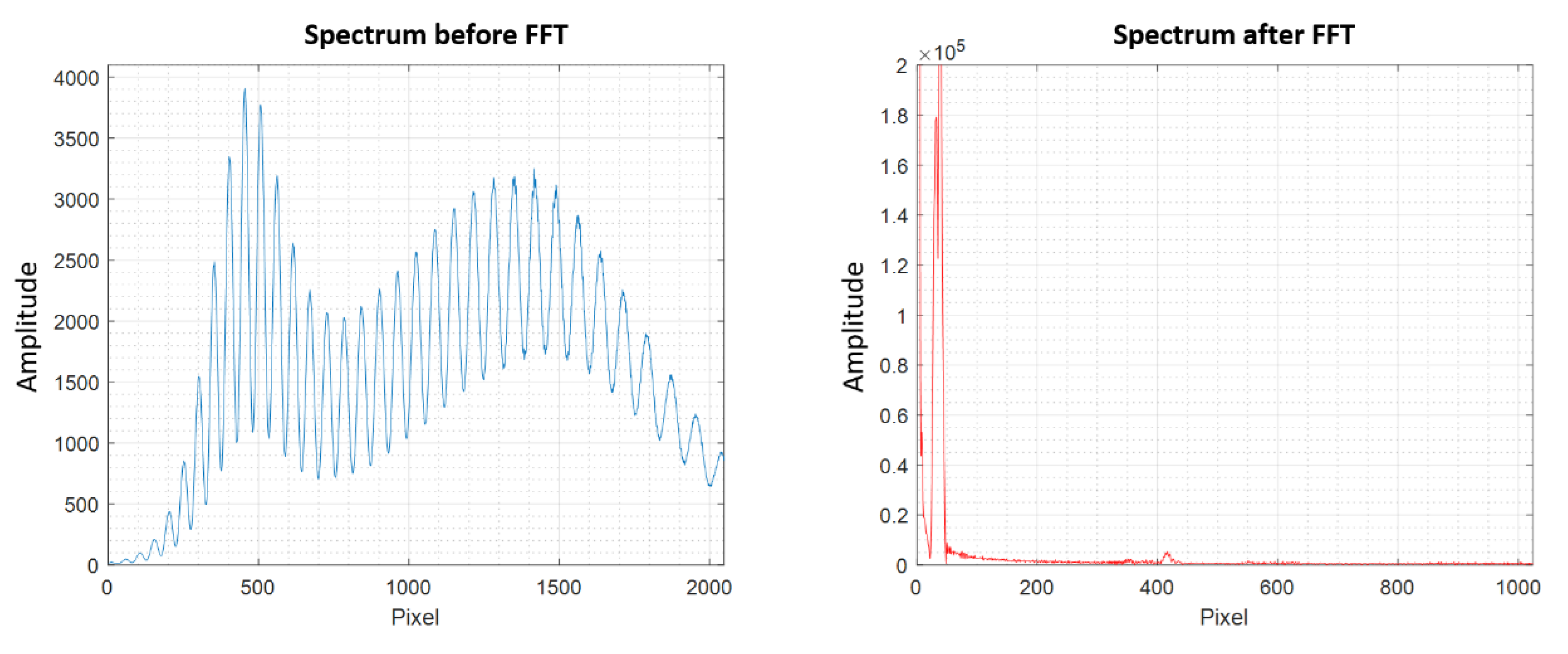
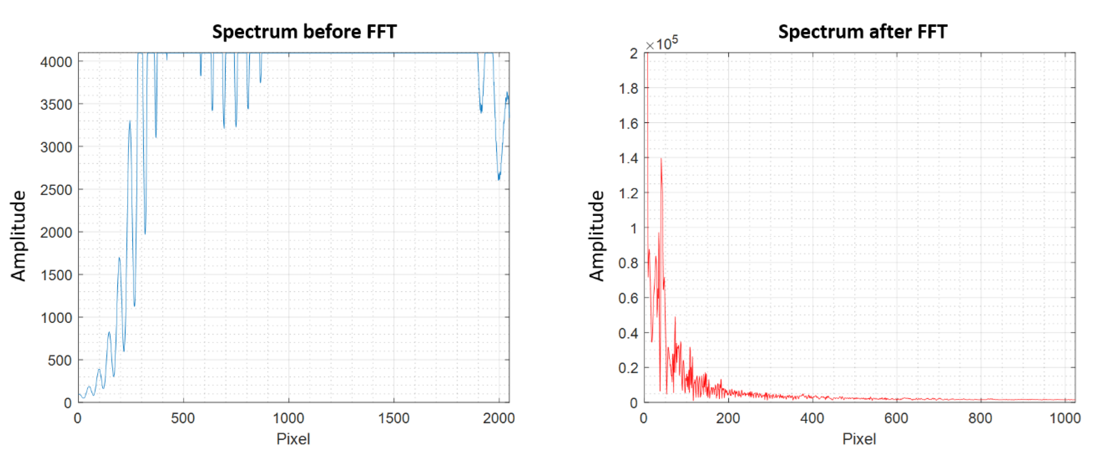
In order to perform a system characterization, it must be ensured that the intensity of light arriving at the line camera in the spectrometer does not lead to an overexposure of this sensor, see Figure 3. This overexposure would make the obtained results unsuitable. At the same time, throttling the output power of the light source leads to a changed spectrum and to a change in the optical properties of the system.

To avoid this, a Thorlabs V800A fiber optic attenuator (FOA) was installed directly after the light source, which allows the output power to be attenuated without changing the spectrum of the light. An overload of the sensor in the spectrometer, as shown in the left picture in Figure 3, leads to the fact that the Fourier transformation cannot determine the frequency spectrum correctly, ghost frequencies are present, shown in Figure 3 on the right side. The result is not usable, because no utilizable information is available. By throttling the FOA, the amount of light is reduced so that the full dynamic range of the spectrometer can be used and thus the spectrum is correctly resolved by the Fourier transform. The degree of this throttling depends on the material to be measured. Since this provides a usable result in the Fourier transformation, the peak in the spectrum generated by the surface can now be identified and later translated into a valid distance information. This ensures that the peak produced by the surface can be detected clearly and correctly later on, see Figure 4.

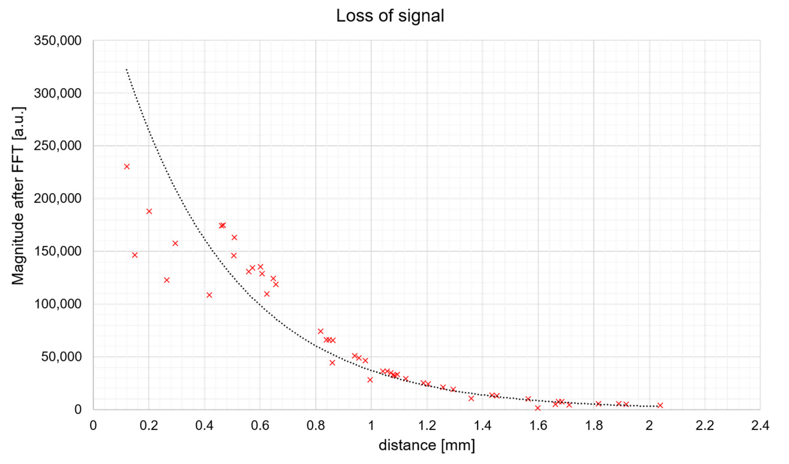
A plane mirror is used to determine the measuring range of the system. This mirror is located in the focal point of the objective and on a piezo stepper, which can move the mirror in vertical direction. The piezo stepper (Physik Instrumente (PI) N-381.3A) used here has a maximum travel of 30 mm, with a resolution of 20 nm. This means that both the travel and the resolution are at least one order of magnitude better than the system can theoretically perform.

The mirror was moved by the piezo stepper with a step size of 0.1 mm and measurements were taken at this position. This process was repeated until the measured signal could no longer be distinguished from the background noise of the sensor due to the distance. The result is that the measuring system has an axial measuring range of 2.3 mm and is therefore large enough to measure the defined structures in the process. In a next step of the calibration the axial resolution of the measuring system was determined and a correlation between a measured height and the position of a peak was derived. According to DIN 32 877 a random position was approached and the position of the resulting peak of the surface was recorded. A total 50 measuring points within the measuring range were considered. By changing the height of the piezo stepper, the position of the peak in the evaluation domain is changed so that a calibration factor can be determined. By dividing the respective difference between the current and previously approached measuring point Z and the corresponding peak positions P, a factor can be calculated. The arithmetic mean is then calculated over the total number of measurements N, see Figure 5.

$$\frac{1}{N}{{\displaystyle \sum }}_{n=1}^N\frac{\left|Z_n-Z_{n-1}\right|}{\left|P_n-P_{n-1}\right|},$$

(4)

The result of this calculation is the experimental determination of the axial resolution of the measuring system for a boundary layer. On the basis of the measurement performed, the following results are obtained for the system: A smallest possible distinguishable step size of 3.632 µm with a local repeatability of 0.36 µm. The calculated axial resolution of the system is 3.318 µm with the parameters of the light source used. The real system can only solve structures that are about 10% larger than those determined in advance. Again, it should be mentioned that this case is valid for tomographic structures, which are not considered here. Despite this deviation, the system has a local repeatability of 0.36 µm and is able to resolve the topographical structures required in the project, like mentioned above. Determining a relationship between the tomographic resolution and the repeatability is part of current research activities.

With the offline laboratory system, it could be shown that the developed measuring system is able to resolve the necessary structures and that the interaction of all components works. In the next step, the upscaling for the actual target application, the laser processing system, can take place.

4. Upscaling to Real World Components

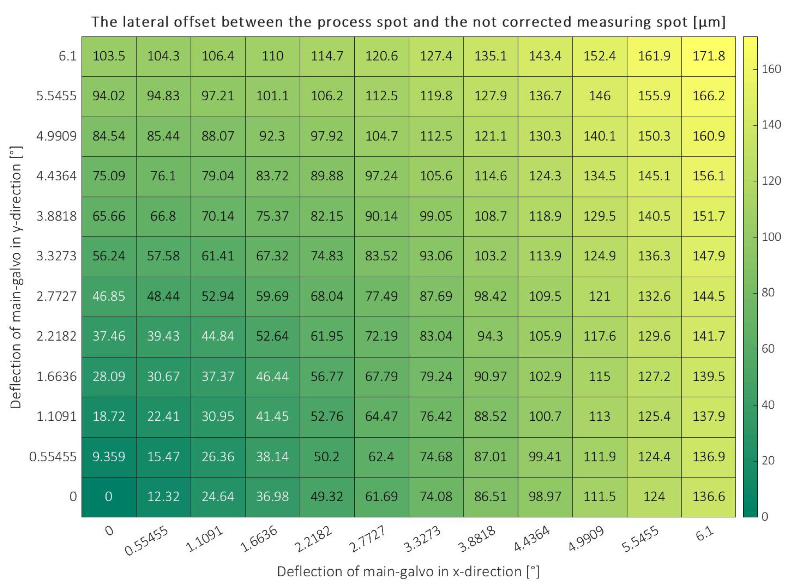
As described above, a different wavelength is used for the measurement system than the design wavelength of the optics. This results in a spot offset in the focal plane, since the objective lens used here is not designed for a wavelength nearly 100 nm different from the process laser. As shown in Figure 6, the positioning error increases the further the beam is deflected. For the lens considered here, the maximum spot offset is 171.8 µm. No direct measurement of the laser ablation is possible. Now it is possible to adjust the machining process to correct the offset. This requires an interruption of the machining process and a repositioning of the scanner mirrors, which would lead to a significant slowdown of the entire process. Another possibility would be to determine a correction file for the scanner objective lens system and the measuring wavelength, as it is used for image field calibration with the process laser. However, this would require significant changes to the process. In addition to the actual processing and the necessary extension for synchronization with the measuring system, a change of the correction data and a repositioning of the scanner would have to take place for each individual measurement in order to be able to measure the same location.

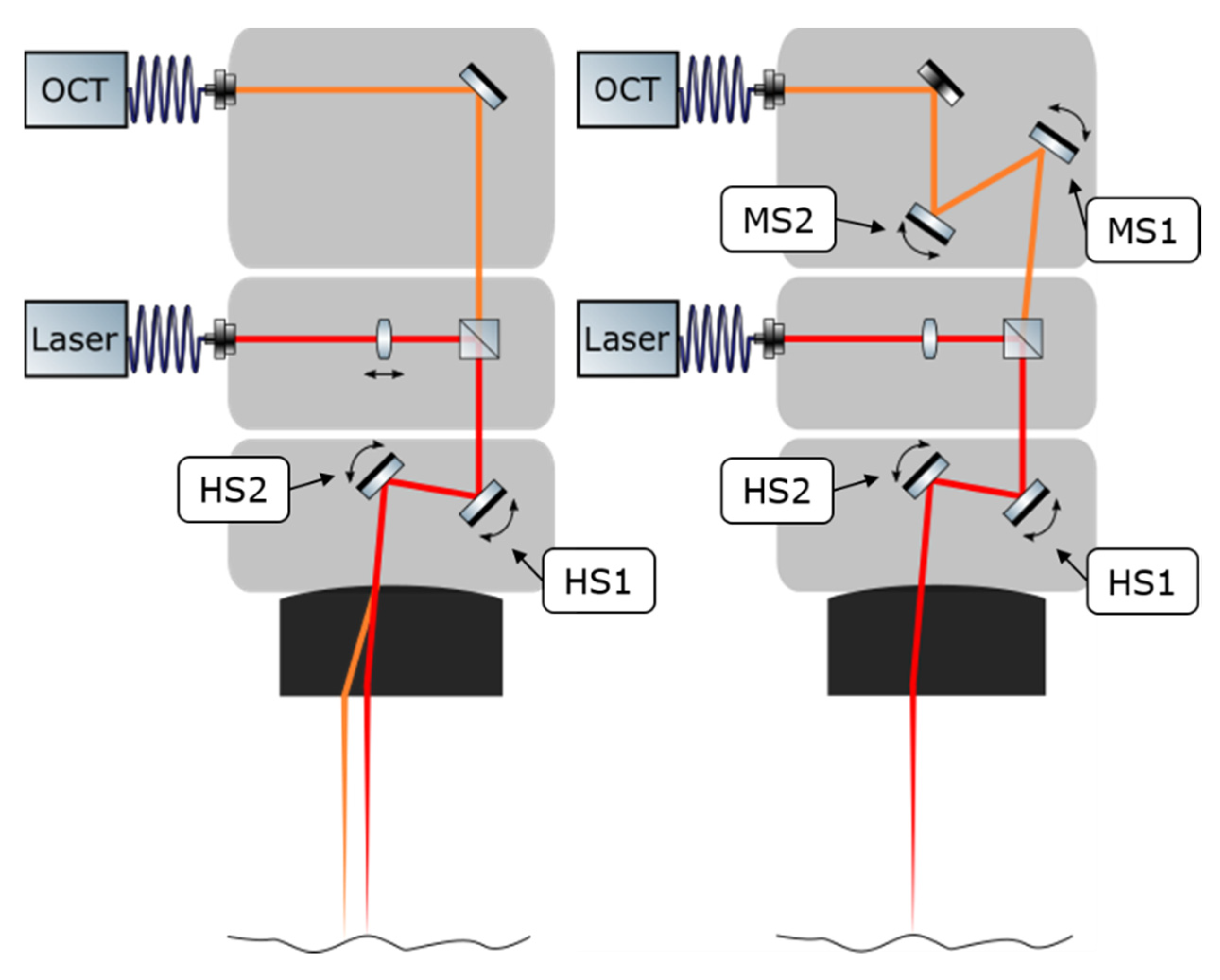
As shown in Figure 7, the spot offset to the border of the objective lens increases. This non-linear or non-constant offset cannot be compensated by additional optical elements, for example, so that a dynamic control is necessary. This dynamic control was made possible by adding another scanner exclusively for the measurement system. As illustrated in Figure 7. At the same time, this opens up new possibilities for process monitoring. It is not only possible to inspect the ablation point, but also a upstream or downstream inspection of the workpiece while the process is running.

5. Spot Shift Compensation Model

The possibility to manipulate the spot position of the measuring system alone is not sufficient to achieve synchronous operation of both systems involved in a production environment. To dynamically adjust the spot position of the measuring system so that overlaying between the process laser and the measuring beam occurs, it is necessary to know the tilting angle of the scanner mirrors required for correction.

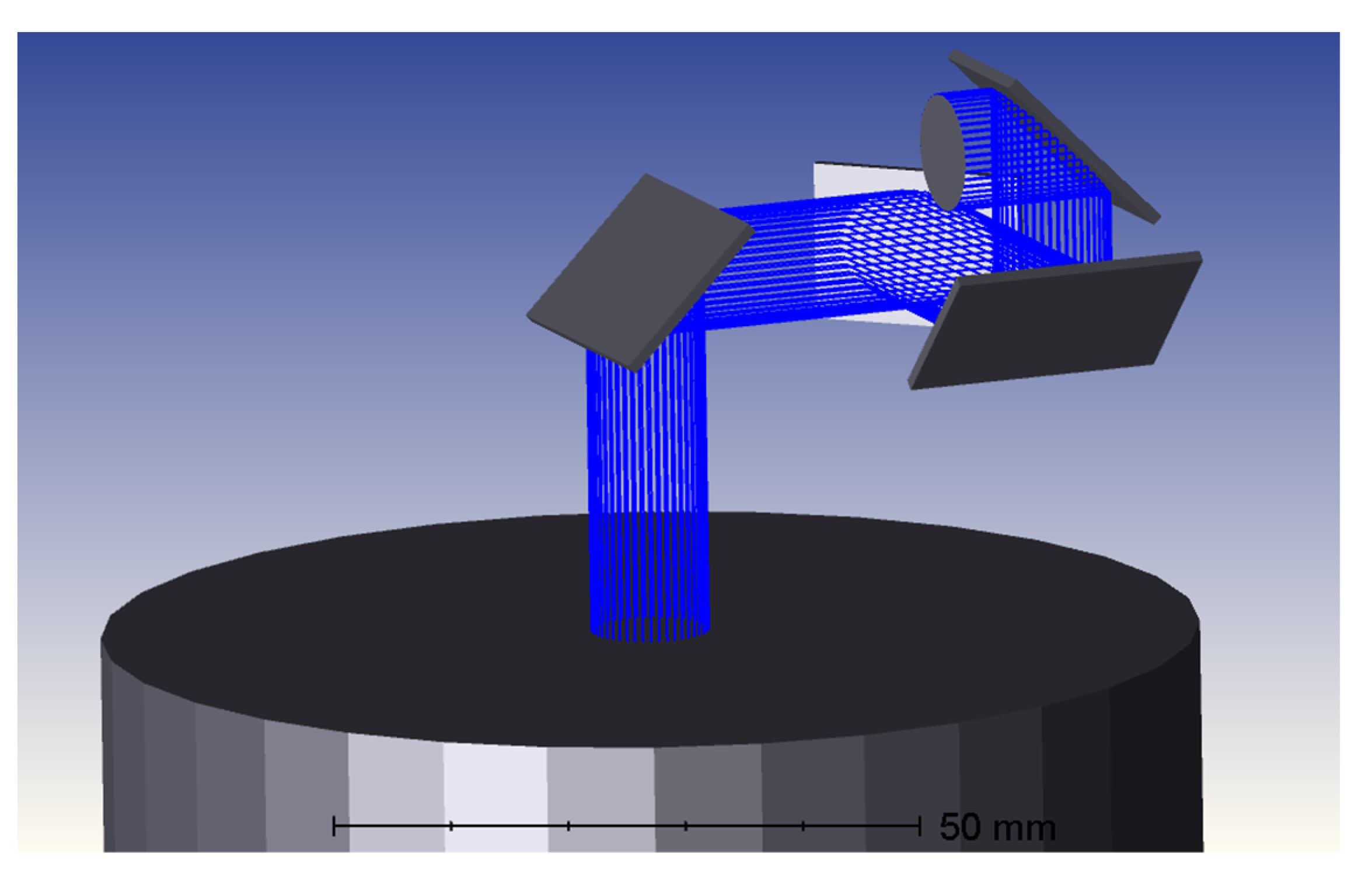
The optical system was recreated as a Zemax OpticStudio simulation and simulated for the outermost point in the image area of the lens, like shown in Figure 8. If both mirrors of the processing scanner (HS1, HS2 in Figure 7) are deflected to the maximum possible angle of [6.0°,6.0°] for the lens-scanner combination, the result is a sport offset of 171.8 µm. Now the mirrors (MS1 and MS2) are varied in 0.001° steps until the optimum is found. As a result, the spot offset in the simulation could be corrected to 1.8 µm or by 98.9%. Thus, a correction on this basis is possible.

However, manual correction is very labor- and time-intensive.

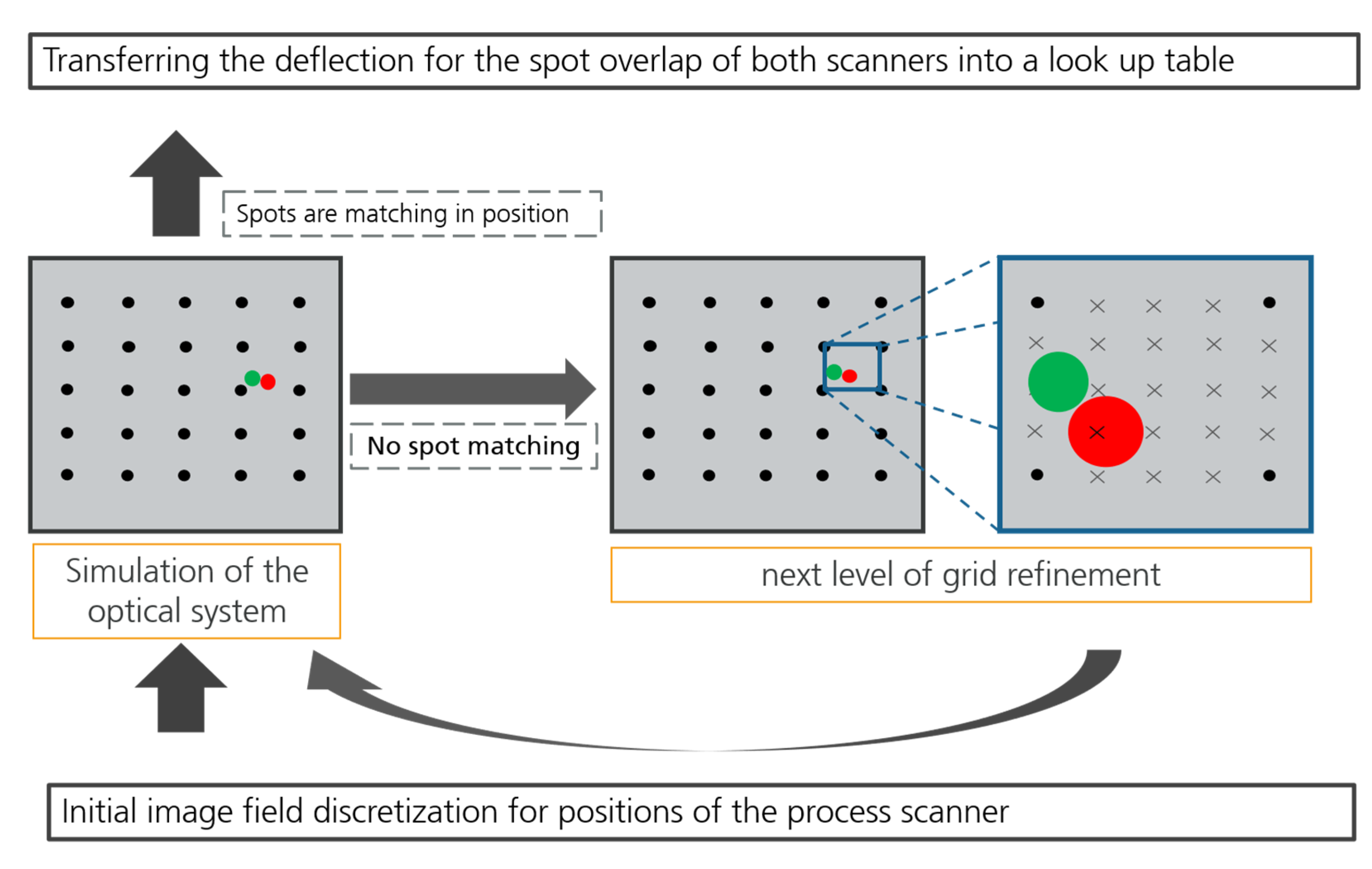
It is difficult to determine all possible combinations of angles and resolutions in advance. A simulation algorithm was developed to obtain correction data for arbitrary discretization, hereby, the density of the generated data point on the surface or the amount of data can be influenced. From the simulation of the light beam path, it is known that the measuring spot is smaller in the focus plane than the processing spot. This is sufficient as a boundary condition for the termination condition of the simulation that the spots cover each other and not that the centers must match.

The aim of the data obtained from the simulation model is to generate a correction table or lookup table in which the angles to be set are dependent on the position of the main scanner. At the same time, the amount of data should be as small as possible. On the one hand, this saves time when generating the data, and on the other hand, it reduces the amount of memory required. For this purpose, the scan field is first assumed to be symmetrical, i.e., the values of one quadrant are transferable to the others, thus reducing the data requirement by 75%. The remaining scan field is now discretized in x- and y-direction, whereby the simulation model enables a flexible and independent discretization of the two directions. The actual calculation of the correction values is now carried out on the points created in this way. In the process, the above-mentioned Zemax OpticStudio simulation was extended so that it can run automatically. Several cycles of the simulation are run through. With each cycle, the step size of the angular iteration is reduced until it reaches the mechanical resolution of the galvanometer used. This procedure is illustrated in Figure 9.

With the data generated in this way, compensation can take place, but due to the discretization, the grid has gaps. These gaps can be closed by interpolating the data. The laser processing system informs the measuring system of the current position of the main scanner and thus the position at which the measurement is to be made. Scanning systems do not usually work directly with the applied angles, unlike our simulation data. Therefore, the first step here is homogenization. Subsequently, the next interpolation points that are located at the adjacent position are identified and the required values are interpolated. The mechanical resolution of the galvanometer used is also taken into account and, if the tolerance is exceeded, the calculation is carried out again with modified interpolation points. As a result, the angles to be created for the scanning system of the measuring system are now available. Now the actual measurement can take place.

During the calibration of the measuring system, the data for the correction table is calculated and transformed into a coordinate system suitable for the scanner used. Thus, the calculation effort during the actual process is limited to the interpolation of interpolation points based on the correction table. Communication between the machining process and the measuring system is required so that the results can be taken, and the spot position of the measuring system can be corrected. LCI as a point-based method requires triggering of each individual acquisition. For this purpose, the machining process must be adapted so that a measurement is triggered at the desired acquisition time, e.g., by a TTL signal, and at the same time it is necessary that there is no movement of the scanner mirrors at the time of the measurement. In order to correct the sport offset, the current position of the processing scanner must be communicated to the measurement system as an extension of the classical LCI. Then the corresponding value for compensation can be applied from the correction model to the additional galvo pair and the actual measurement can take place. These two steps must be integrated into the actual machining process for the locations for which a measurement is to be made so that accurate results can be obtained.

The simulation model is designed in such a way that optical or mechanical components can be exchanged, e.g., for adaptation to a different setup.

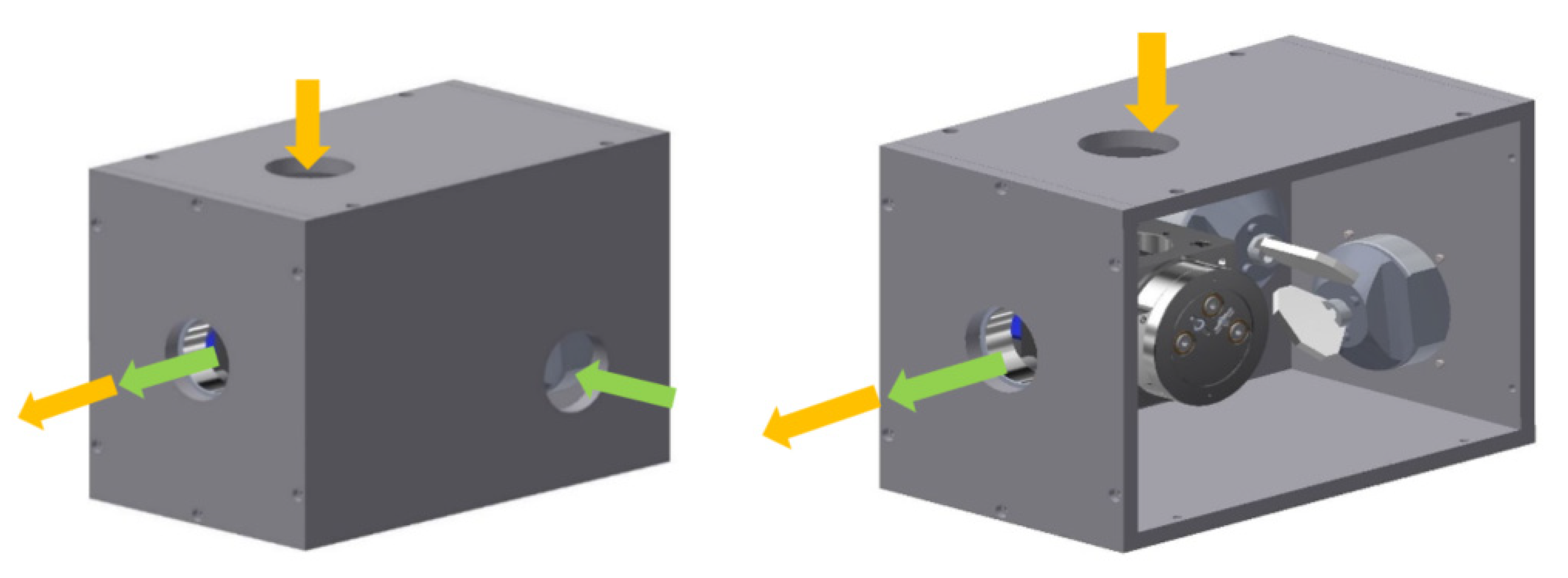
New challenges arise here during integration into the laser machine. In order to be able to accommodate the second scanning system in the laser machine, it is necessary to develop an integration box, shown in Figure 10. This is used to couple the processing laser into the beam splitter and at the same time the scanner unit for the measuring system is housed here and also coupled into the beam path of the machine via the beam splitter. Only the beam splitter has been integrated as a new component in the beam path of the process laser and it has only the influence of a mirror.

This is used to couple the processing laser into the beam splitter and at the same time the scanner unit for the measuring system is housed here and also coupled into the beam path of the machine via the beam splitter. Only the beam splitter has been integrated as a new component in the beam path of the process laser.

6. Discussion and Conclusions

The measurement system based on low coherence interferometry described here enables measurements to be taken directly at the point of ablation. This also requires a new method of controlling the machining process. The necessary synchronization between the machining process and the measurement increases the machining time for a workpiece. The increase in time depends on factors such as the number of measuring points or the possible recording frequency of the spectrometer used and is therefore dependent on the actual process. No removal of the workpiece is necessary, so there is no need for repositioning work. The ablation of a laser structuring process usually takes place in several cycles, with material in the nm range being ablated in each cycle [32]. This is also a limitation of the LCI process, with a repeatability of 0.36 µm an ablation cycle is not detectable, but a set of them. If the workpiece is inspected at the end of the machining process to determine target parameters or to adjust process parameters, the resulting delay is much smaller than if each cycle of the process is measured. If the machining process runs without the use of the measuring system, there is no delay or further influence on the process.

The basic challenge of the spot offset was solved by integrating a separate scanner for the measuring system and a model for control. This integration also opens up new application possibilities. In this context, the goal was to achieve a spot overlap, which was successfully achieved with the control model. The model can be adapted to other optical systems. The generation of the correction data is very complex. There is a need for further research to reduce the amount of data and to find a more effective way to integrate the control into the process [33]. The independent control of the measuring and processing beam allows further investigations of the measuring strategy. For example, the measuring spot can be positioned in front of or behind the ablation point and new process data can be generated or interactions between the measuring light and the plasma created by the ablation can be bypassed. In addition to pure process monitoring, data volumes for AI approaches can also be recorded in this way. Spot offset compensation can be useful not only in the topographical case discussed here, but also in the application of classical OCT, e.g., for process monitoring in laser transmission welding [34]. However, further research is needed on these points.

With the methods presented here, an extension of the LCI by a sport offset compensation was made and the system was developed to meet the specific project requirements. It could be shown that the target structures can be solved, and how a spot offset can be compensated, or which mechanical adjustments have to be made for a system integration into an existing machine. As the ESSIAL research project is still ongoing, the presented method will be further developed and adapted if necessary.